Article

CFD-CNN Modeling of the Concentration Field of Multiport Buoyant Jets

1
School of Water Resources Engineering, Dalian University of Technology, 2 Linggong Road, Dalian 116024, China
2
Key Laboratory of Hydrometeorological Disaster Mechanism and Warning of Ministry of Water Resources, Nanjing University of Information Science & Technology, Nanjing 210000, China
3
Department of Civil Engineering, University of Ottawa, Ottawa, ON 999040, Canada
*
Author to whom correspondence should be addressed.
J. Mar. Sci. Eng. 2022, 10(10), 1383; https://doi.org/10.3390/jmse10101383
Submission received: 21 July 2022 / Revised: 6 September 2022 / Accepted: 22 September 2022 / Published: 27 September 2022
(This article belongs to the Special Issue Advances in Coastal Hydrodynamics and Water Quality Modeling)

Abstract

:
At present, there are increasing applications for rosette diffusers for buoyant jets with a lower density than the ambient water, mainly in the discharge of wastewater from municipal administrations and sea water desalination. It is important to study the mixing effects of wastewater discharge for the benefit of environmental protection, but because the multiport discharge of the wastewater concentration field is greatly affected by the mixing and interacting functions of wastewater, the traditional research methods on single-port discharge are invalid. This study takes the rosette multiport jet as a research subject to develop a new technology of computational fluid dynamics (CFD) modeling and carry out convolutional neural network (CNN) simulation of the concentration field of a multiport buoyant jet. This study takes advantage of CFD technology to simulate the mixing process of a rosette multiport buoyant jet, uses CNNs to construct the machine learning model, and applies RSME, R2 to conduct evaluations of the models. This work also makes comparisons with the machine learning approach based on multi-gene genetic programming, to assess the performance of the proposed approach. The experimental results show that the models constructed based on the proposed approach meet the accuracy requirement and possess better performance compared with the traditional machine learning method, and they can provide reasonable predictions.

1. Introduction

Wastewater discharge is an important factor that leads to changes in the water environment, which can not only change the physicochemical property of water but can, worse still, also cause the pollution of water, eutrophication, and so on. Therefore, it is of great importance to study the mixing mechanism of wastewater discharge. When the density of wastewater and the receiving water are different, the motion forms a buoyant jet [1]. To protect the quality of the near-shore water environment, wastewater produced by municipal administration and sea water desalination is often dealt with as offshore discharge. This means the wastewater is taken through the discharge system to the diffuser and centralized discharger. The choice of diffuser type is one of the important influencing factors affecting the sewage discharge density field [2]. The commonly utilized diffusers are single-hole-type, T-type, rosette diffusion-type, and so on; the single-hole type is seldom utilized in actual sewage discharge projects because of its slow speed and limited dilution capacity. The rosette-type diffuser has the features of small spacing, low price, and strong dilution capacity, and is extensively utilized in sewage discharge. However, on account of its complex mechanism, the modeling of the sewage mixing procedure in the discharge procedure of rosette-type diffusers is relatively inefficient, so further research is needed.
Physical modeling and experimental methods are the most used methods to study rosette jets. For example, Lai and Lee [3] published measurement trajectories of jets discharged from rosette-like diffusers to stagnant water, Abessi et al. [4] measured the mixing process of rosette-dense jets in fixed receiving water, and Abessii and Roberts [5] reported concentration field measurements of rosette-dense jets in flows. These previous experimental works have greatly improved the knowledge of rosette jets. However, laboratory methods are often very time-consuming and expensive, so there is an urgent need to develop complementary methods [6]. On account of the significant elevation of computer speed and storage capacity, especially the rapid development of computer-generated three-dimensional mesh capabilities, computational fluid dynamics (CFD) applications are becoming more and more extensive [7]. CFD mainly studies and describes various flow phenomena [8] and can use computers instead of physically simulating the natural environment, mechanical devices, and so on, so the CFD model is utilized to study the jet and realize its three-dimensional numerical simulation [9]. As a complement to physical modeling and experimental approaches, several studies on the analysis or simplified numerical models of unidirectional multi-femoral jets have been reported. Yannopoulos et al. [10] experimented with a circular vertical turbulent buoyancy jet, using tap water as a jet liquid and saline as an environmental liquid, analyzed the normalized axial velocity and concentration distribution along the jet axis, and proved that the research results could be used for design purposes, laboratory simulation study, and numerical model verification. Wang et al. [11] discussed the interaction between jets in stationary fluids and their adjacent jets, established a model of an infinite-length isometric identical jet merger in stationary fluids, and successfully predicted the diffusivity change in the free entrainment and jet merger planes, as well as the tracer distribution during the merger process. However, the CFD method requires a significant amount of memory as well as computation time, so further research should be carried out to improve forecasting and computing power, and shorten the time required [12]. Currently, machine learning has been extensively utilized in the field of water conservation, and the applicability of the model has been proven in practice. Therefore, machine learning can be combined with computational fluid dynamics to train predictive models. Compared with traditional regression-based methods, machine learning does not require a predetermined structural model, has portability, discovers the internal distribution characteristics of the data through neural networks, and quickly and directly obtains the hidden relationship between the input layer and the output layer. Therefore, machine learning-based models are often superior to empirical equations derived using traditional regression-based methods. Methods based on ML can be divided into direct and indirect methods. In the direct method, the ML-based model is developed for target variables such as flow rate, water depth, and flood range. For example, Yan et al. [13] predicted the flow depth of river systems using the polygenic genetic programming (MGGP) method. We will show that the ML algorithm can effectively replace the hydraulic model and significantly reduce the computational cost. In indirect methods, the ML algorithm is used to develop new lower-order models of turbulence closure or flow simulations. For example, Zhao et al. [14] proposed a CFD-driven ML method for the development of the Reynolds-Average Navier–Stokes (RANS) model. Compared with the simple CFD model, the trained CFD model based on machine learning shows good efficiency [15,16] and good practicality [17,18]. The training procedure of machine learning techniques often requires large datasets, but large amounts of data are often not available in the water conservation field, which limits its widespread use in water-related problems.
This study aims to develop a CFD and machine learning-based model to simulate rosette multiport sewage discharge. Firstly, the CFD model is utilized to simulate the mixing procedure of the buoyant jet discharged by the rosette multiport diffuser, and the experimental data are verified. After the verification is passed, additional calculations are made using the CFD model to enrich the dataset and meet the requirements of machine learning, which requires a large amount of data. The result is a machine learning model that can be trained by an extended dataset. It predicts standardized concentrations at diverse locations of the discharge holes. In this study, CFD models are built within the framework of OpenFOAM [19], and machine learning models are developed using convolutional neural network (CNN) methods [20,21]. An important outcome of this study is a trained hybrid model based on CFD and machine learning [22]. The hybrid model based on CFD and machine learning has the same accuracy as CFD models, but has been greatly improved in computational speed, enabling predictions to be carried out in seconds. Unlike the previous CFD model in the application of jets, most of the previous research was mainly utilized to develop and evaluate the performance of diverse models, and this study uses CFD models to expand the dataset for the purpose of providing a large amount of data for machine learning.
Machine learning was utilized for sewage discharge modeling, while the mixing mechanisms for diverse types of discharges are significantly distinct, and the prediction performance of diverse technologies is also distinct. For the purpose of improving the efficiency of machine learning and verifying the modeling effect of CNNs, this machine learning uses convolutional neural networks for modeling. In previous research work, authors have modeled rosette-type multiport emissions using polygenic genetics (MGGP) techniques. The overall idea of the MGGP algorithm is based on Darwin’s law of biological evolution of “survival of the fittest”. It integrates the concepts of gene coding, chromosome crossover, gene variation, and natural selection in biology into the procedure of optimizing the solution of the problem, and finally obtains the optimal solution to the problem through continuous “population evolution”. While MGGP modeling has the disadvantages of complex genetic algorithm programming, involving gene encoding and decoding, setting parameters such as crossover rate and the variability contained in the algorithm relies on experience and a strong dependence on the advantages and disadvantages of the initial population. CNNs are structures that mimic human nerves and consist of neurons with learnable weights and bias constants. CNNs have the advantages of sharing convolutional kernels, having no pressure on high-dimensional data processing and the ability to retain the original position relationship after the image is convoluted, among other things. Recently, the CNN algorithm has been widely used in the field of water resources research and has proven to be an effective tool for predicting complex water-related processes. For example, Eltner et al. [23] proposed a new method of automatically measuring water levels through CNNs and photogrammetry. The results showed that the proposed method can provide reliable water level measurements. Recent studies have shown that the CNN algorithm can effectively predict flow fields, and Kreyenberg et al. [24] measured concentration distribution based on the density-driven solute transport, using CNNs to estimate the velocity field. The results showed that the CNN algorithm can successfully represent the underlying mechanism and compensate for the information difference of the missing system variables. Therefore, by comparing the modeling results of the MGGP and CNN methods, starting from the mean square value and concentration distribution map, this paper verifies that the CNN method has great advantages in processing spatial data; as far as the authors are aware, this is the first time that three-dimensional computational fluid dynamics and CNNs have proposed the technology for developing a rosette-type multi-port buoyancy emission model.

2. Materials and Methods

2.1. CNN Method

The convolutional neural network is a multi-layer supervision learning neural network, and the convolutional layer and pool sampling layer of the implicit layer are the core modules that implement the feature extraction function of the convolutional neural network. Convolutional neural network structures include the convolutional layer, the down sampling layer, and the fully linked layer. Each layer has multiple feature maps, each feature map extracts the input of a feature through a convolutional filter, and each feature map has multiple neurons. Convolutional layer: Because we can extract the characteristics of the data through convolution operations, we can enhance some of the characteristics of the original signal, and reduce noise. Down sampling layer: Because conducting down sampling on the image can reduce the amount of data processing while retaining useful information, sampling can confuse the specific position of the feature, and because, after a feature is found, its position is no longer important, we only need the relative position of this feature and other features, and this can cope with the changes of the same kind of objects brought about by deformation and distortion. Fully connected layer: Softmax is utilized to fully connect, and the obtained activation value is the picture feature extracted by the convolutional neural network. A convolutional structure can reduce the amount of memory occupied by the deep network, and it has three key operations: one is the local sensing field, the other is weight sharing, and the third is the pooling layer, which effectively reduces the number of parameters of the network and alleviates the overfitting problem of the model. The network model uses the gradient descent method to minimize the loss function to reverse adjust the weight parameters in the network layer by layer, and this improves the accuracy of the network through frequent iterative training. Its weight-sharing network structure makes it more similar to biological neural networks, reducing the complexity of network models and reducing the number of weights. This advantage is more obvious when the input of the network is a multidimensional image, so that the image can be directly utilized as the input of the network, avoiding the complex feature extraction and data reconstruction procedure in the traditional recognition algorithm [25]. Deep CNN is specialized in processing 2D data (images and videos), commonly referred to as “2D CNN”. 2D CNN can extract features from massive, labeled data and learn complex objects. Although the classical CNN was developed specifically for 2D signals, Kiranyaz et al. [26]. proposed the first 1D-CNN to process sequential data (1D signals). Since then, 1D CNN has been widely and successfully used in various fields, such as biomedical data classification (Zihlmann et al., 2017) [27] and structural damage detection (Abdeljaber et al., 2018) [28].
In essence, CNN is an input-to-output mapping that learns a significant amount of mappings between inputs and outputs without the need for any precise mathematical expressions between inputs and outputs, and as long as convolutional networks are trained with known patterns, the network has the ability to map between input and output pairs. The training procedures for the network are as follows:
(1)
Select the training group and randomly set 60 percent of the samples as the training group, 20 percent as the verification group, and 20 percent as the test group from the sample set;
(2)
Set each weight and threshold value to a small random value close to 0 and initialize the precision control parameters and learning rate. Set the parameter epochs to 1000, batch size to 32, and verbose to 2;
(3)
Select Fr, x, and y as the input vectors, and normalize the concentration target output vector;
(4)
Calculate the output vector of the middle layer and calculate the actual output vector of the network;
(5)
The output error is calculated by comparing the elements in the output vector with the elements in the target vector. For the hidden elements of the middle layer, the error also needs to be calculated;
(6)
The adjustment amount of each weight and the adjustment amount of the threshold are calculated in turn;
(7)
Adjust weights and adjust thresholds;
(8)
When M is experienced, it is judged whether the indicator meets the accuracy requirements. If not, it returns (3) and continues to iterate. If satisfied, it proceeds to the next step;
(9)
At the end of training, the weights and thresholds in a document are saved. At this moment, it can be considered that the various weights have reached stability and the classifier has been formed. Training is performed again, exporting the weights and thresholds directly from the documents for training; no initialization is required.
CNNs themselves can take diverse forms of neurons and learning rules, and the generalization ability is significantly better than other methods. Convolutional neural networks have been utilized for pattern classification, object detection, and object recognition. The pattern classifier is established by using the convolutional neural network, and the convolutional neural network is utilized as a general pattern classifier for direct use in grayscale images.

2.2. The Joint Method of CFD-CNN

The method first requires a good CFD model to be built. In previous work, the author utilized the OpenFOAM platform to build a CFD model. First, Spatial analysis of the diffuser is performed to determine the jet influence factors. The multifluid solver “twoLiquidMixingFoam” in the OpenFOAM framework is used to solve the governing equations. Secondly, the grid is established. By dividing the diffuser evenly into 12 parts, to save the computational cost, only one part is simulated, and the rest can be obtained through the “symmetric” and “mirror” functions. The initial jet velocity, Uj, is set to 0.365 m/s, and the density Freud number, Fr, is 2.5 for the baseline case. Non-slip boundary conditions with standard wall functions are assigned to the bottom patch. The jet inlet adopts a fixed value velocity, and the coordinates of the jet inlet (port surface) remain unchanged under different circumstances. The horizontal distance between the jet inlet and the centerline of the computational domain is 0.028 m, and the vertical distance between the jet inlet and the bottom patch is 0.140 m. Computational geometry and meshes were created using the open-source platform, Salome. A locally modified unstructured computational grid near the ports is used for domain discretization. The mesh size is between 0.001 m and 0.005 m. The number of grids is less than 1 million, so the simulation can easily run on a PC. Digital time steps are dynamically determined by the “adjust time steps” code available in OpenFOAM, and the criterion for calculating termination is defined by the user-defined end time. Final numerical simulations of the rosette buoyancy jet experiments, as reported by Lai and Lee [14], are carried out, followed by six calculations using the validated model. The experimental data and predicted data are compared, and the jet trajectory and cross section distribution are verified. The verification results are good and meet the accuracy requirements, so the joint CFD-CNN model will be based on the CFD model previously established. Additional simulations are performed with CFD models to scale datasets for machine learning. Froude numbers are a key factor affecting the mixed diffusion performance of wastewater, so this study uses CFD models to simulate 20 diverse Froude numbers. Because the CFD model has been tested, we believe that the accuracy of the simulated data is acceptable, and it is trained as measured data.
The dataset contains four variables: the number of Fr, x (horizontal) and y (vertical) coordinates, and normalized concentrations. To prevent overfitting, the dataset is divided into training, validation, and testing sets on a 6:2:2 scale. To build a CNN-based rosette buoyancy jet concentration field model, the Number of Fr and x and y coordinates are defined as input variables, and the normalized concentration is utilized as the output variable. First, the training set is utilized for model training, and the validation set validates the trained model. The number of training iterations is set to 1000 generations, and the model is evaluated by RSME, R2 value, etc. If the validation results are good, the prediction is made from the test set. If the verification effect is not good, the parameters are adjusted to continue training.

2.3. Comparison of Models

Multigene Genetic Programming (MGGP) is the development of genetic pattern groups (GP) and combines the model building capabilities of GP with the parameter estimation capabilities of statistical regression methods to find the relationship between input and output variables through a series of procedures [29]. In traditional genetic programming, evolutionary models consist of single chess trees, while in polygenic genetic programming, each regression model is a weighted line combination of multiple pendulum trees [30]. The workflow can be roughly described as follows: random generation of primary populations, consisting of a group of individuals consisting of correspondence and variables; calculating the adaptability of each individual in the population, and selecting the excellent individual with good adaptability as the mother; by means of mutation, intersection, replication, and so on, new individuals are generated and a new generation (offspring) is created; repeating the second step and the third step until the termination criteria are met.
In the previous work, the author utilized machine learning to model the buoyancy jet of the rosette-type diffuser. The authors built the MGGP-CFD hybrid model based on the CFD model [31]. Additional simulations using CFD to extend the machine learning dataset and reuse MGGP for learning ultimately resulted in a predictive model. However, the prediction data obtained from the MGGP model has low accuracy and needs further improvement. For the purpose of verifying the advantages of the CNN modeling results, this research compares the modeling results of MGGP and CNN, two diverse methods from mathematical statistics, normalized concentration distribution, and so on, to determine the advantages and disadvantages of model performance.

3. Results

3.1. Results of CFD

In this research, the multifluid solver “twoLiquidMixingFoam” under the OpenFOAM framework was utilized to solve the control equations. Yan et al. [6] have verified that this model can be utilized for rosette-type multi-port emission buoyancy jets. As shown in Figure 1, The emitter consists of six ports with a diameter of 0.0044 m, and the calculation domain is a cylinder with a diameter of 0.6 m. Because the research area is symmetrical, it can be divided into 12 areas, and for the purpose of saving costs, only one of the areas is numerically simulated, and the entire research area can be obtained by using symmetry. The boundary condition is set for the subdomain, the symmetry plane uses the symmetry boundary, and the bottom adopts the standard wall function without slip boundary condition. The jet inlet uses a fixed value velocity, and in this research the initial velocity in the vertical direction is set to 0. The top and exterior settings are the inlet—outlet boundaries. The “flipped” and “mirrored” images via ParaView (Sandia National Laboratory, New Mexico, USA) and Tecplot software have small and negligible errors. Because the sewage is discharged centrally at the port, an area of 0.06 m times 0.06 m near the port was selected as the area of interest to study the dilution mixing characteristics of the buoyancy jet. The initial values of k and ε ware calculated based on the jet diameter, initial velocity, and initial density, which are 0.000246 m2/s2 and 0.002061 m2/s2, respectively. The open-source platform Salome was used to compute the geometry and meshes, with regional discretization near ports and local refinement using unstructured computational meshes. According to the method proposed by Yan et al. [2], a sensitivity analysis of the grid was carried out, and the grid size iwas finally determined to be between 0.001 and 0.005 m. The “adjusttimestep” in the OpenFOAM software was used to automatically determine the time step.
Numerical simulations were performed for the single discharge ports. Table 1 shows the basic parameters of the simulation. The rosette-type buoyancy jet data obtained by experiments and simulations are shown in Table 2 (The center of the diffuser is taken as the origin, the transverse is the x-axis, and the vertical is the y-axis). From Table 2, it can be observed that the simulated buoyancy jet is a vertical buoyancy jet, and the trajectory of the dilution characteristics is basically consistent with the experiment. The rms error (RMSE) of the normalized concentration is 0.25, the measurement coefficient (R2) is 0.98, and the normalized rms error (NRMSE) is 0.04. The dilution characteristic trajectory of the simulated jet on the vertical cross-section at diverse heights is also basically consistent with the experiment. Therefore, we believe that the model meets the accuracy required for simulation, can simulate the buoyancy jet relatively well, and can reasonably predict the dilution characteristics of a buoyant jet of the rosette-type multi-port diffuser.
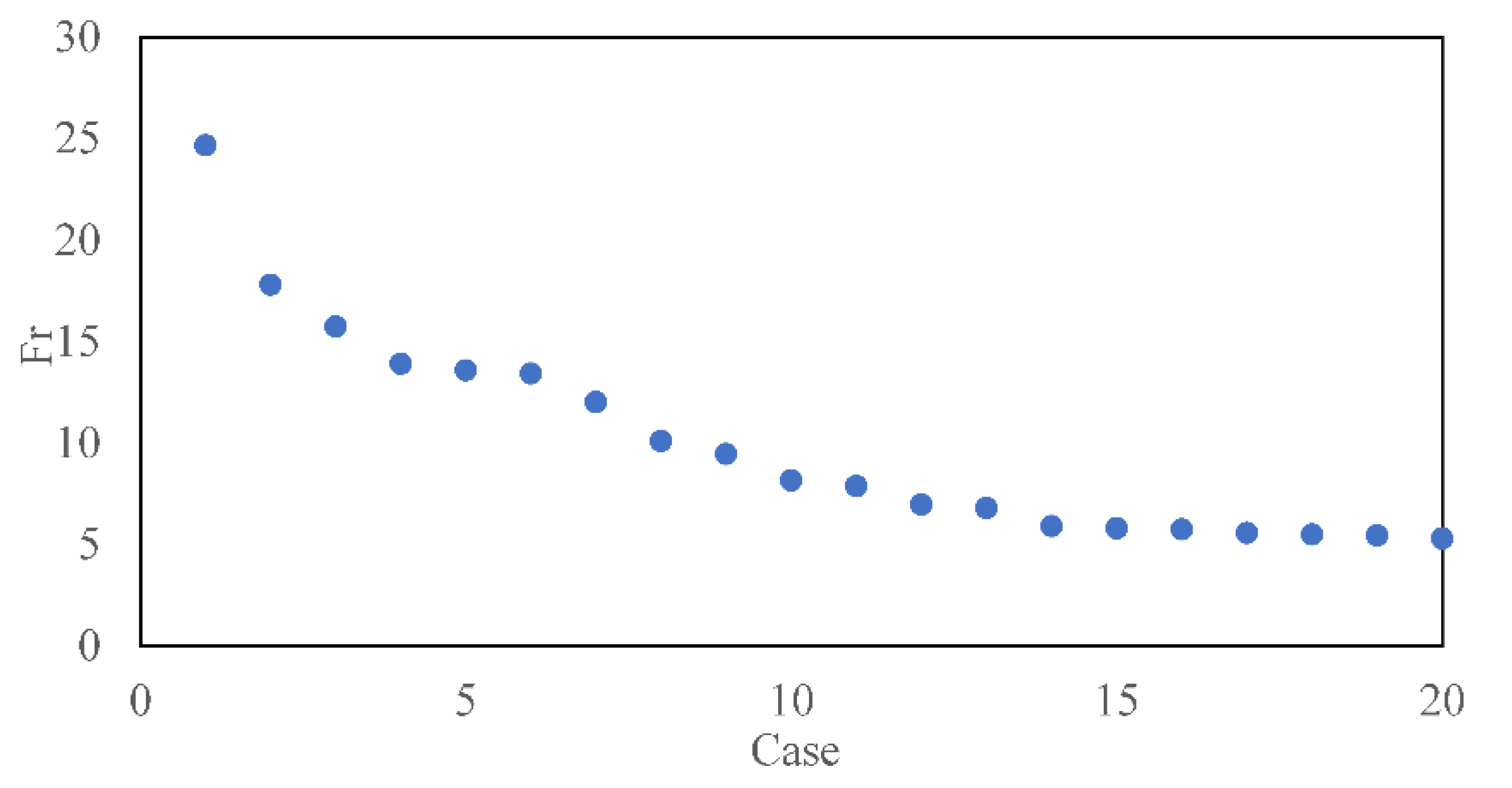
Froude number is an important factor affecting the mixed characteristics of buoyant jets. Therefore, in this study, 20 jets with diverse Fr values were simulated using the above validated CFD model, as shown in Figure 2. In various cases, the initial velocity, jet angle, sewage density, etc. are the same. The ambient water density value is determined using the “rand” function in MATLAB, and the Fr value is randomly selected, with a maximum of 24.676 and a minimum of 5.750. Because Fr is not very diverse in diverse cases, it is believed that the current number of cases meets the data requirements of the machine learning training model. The default value utilized for calculating the time step is 1 s, but the model automatically adjusts based on the Courant number, which has a value of 1. Sensitivity analysis was performed to finally determine that the simulation run time was 30 s, and the longer calculation time did not have a significant impact on the results. Figure 2 shows the Froude parameters for 20 cases.
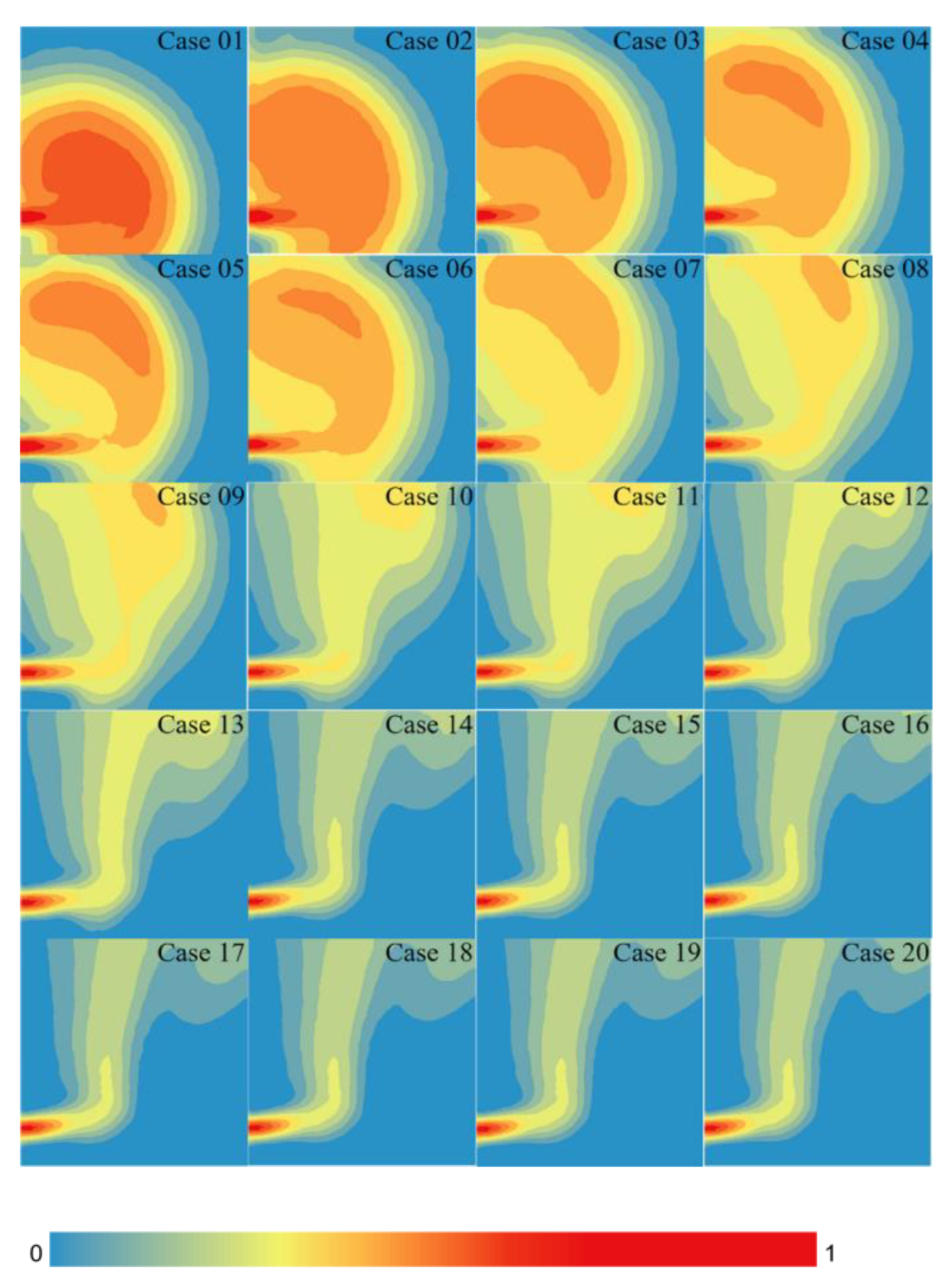
Figure 3 shows the jet dilution trajectory of 20 cases under the CFD model, using the normalized concentration at the center plane (shown in the dashed line in Figure 1b) (defined by concentration, C, divided by the initial jet concentration, C0) to represent the concentration size near the port. As can be observed from the figure, the influence of the Froude number on the dilution trajectory of the jet is very significant. The jet is generally a vertical buoyant jet, diluted by the discharge port, and the farther away from the port, the lower the concentration and the greater the diffusion range. The smaller the Froude number, the larger the difference in the density of sewage and environmental water, the greater the buoyancy effect, and the more obvious the vertical upward layering. In addition, the influence range is above the port, showing a parabolic shape. On the contrary, the smaller the Froude number, the smaller the difference in the density of sewage and environmental water, the smaller the buoyancy effect, and the less obvious the stratification. The diffusion impact range at the port is approximately circular, the concentration near the discharge fracture does not change much, and the bending is not obvious. The smaller the difference in Froud’s numbers, the less diverse the jet concentration curve is.
Numerical data were extracted using ParaView and MATLAB, and in the dataset the mean, minimum, maximum, and median values of Fr were 9.993, 5.305, 24.676, and 8.022, respectively. The standard deviation, variance, kurtosis, and bias were 5.079, 25.801, 4.109, and 1.267, respectively. The mean, minimum, maximum, and median values of the normalized concentrations were 0.33, 0, 1, and 0.28, respectively. The standard deviation, variance, kurtosis, and skewness of the normalized concentrations were 0.28, 0.08, 2.09, and 0.49, respectively. Because this model has been validated, the above 20 cases were utilized as measured data for training and testing machine learning models.

3.2. Results of CFD and CNN Joint Method

While applying the MGGP method to train a model, 80 percent of the data were utilized to train the model, and 20 percent were utilized to test the model. The training procedure was set to 1000 generations; each generation could generate 500 models, and the model performance was evaluated by the RSME value. During training, the model performance was more obvious. At the beginning of training, the model performance was poor, and the RSME value was large, averaging about 0.3. With the training, the model performance improved; after approximately 300 generations, the difference was small; RSME value was lower than 0.15. For the purpose of ensuring the accuracy of the model, learning was continued to 1000 generations. The last generation of models trained by MGGP consisted of 500 models, which needed to be evaluated for better accuracy and simpler operation, and the best model was selected through the Pareto-optimal method.
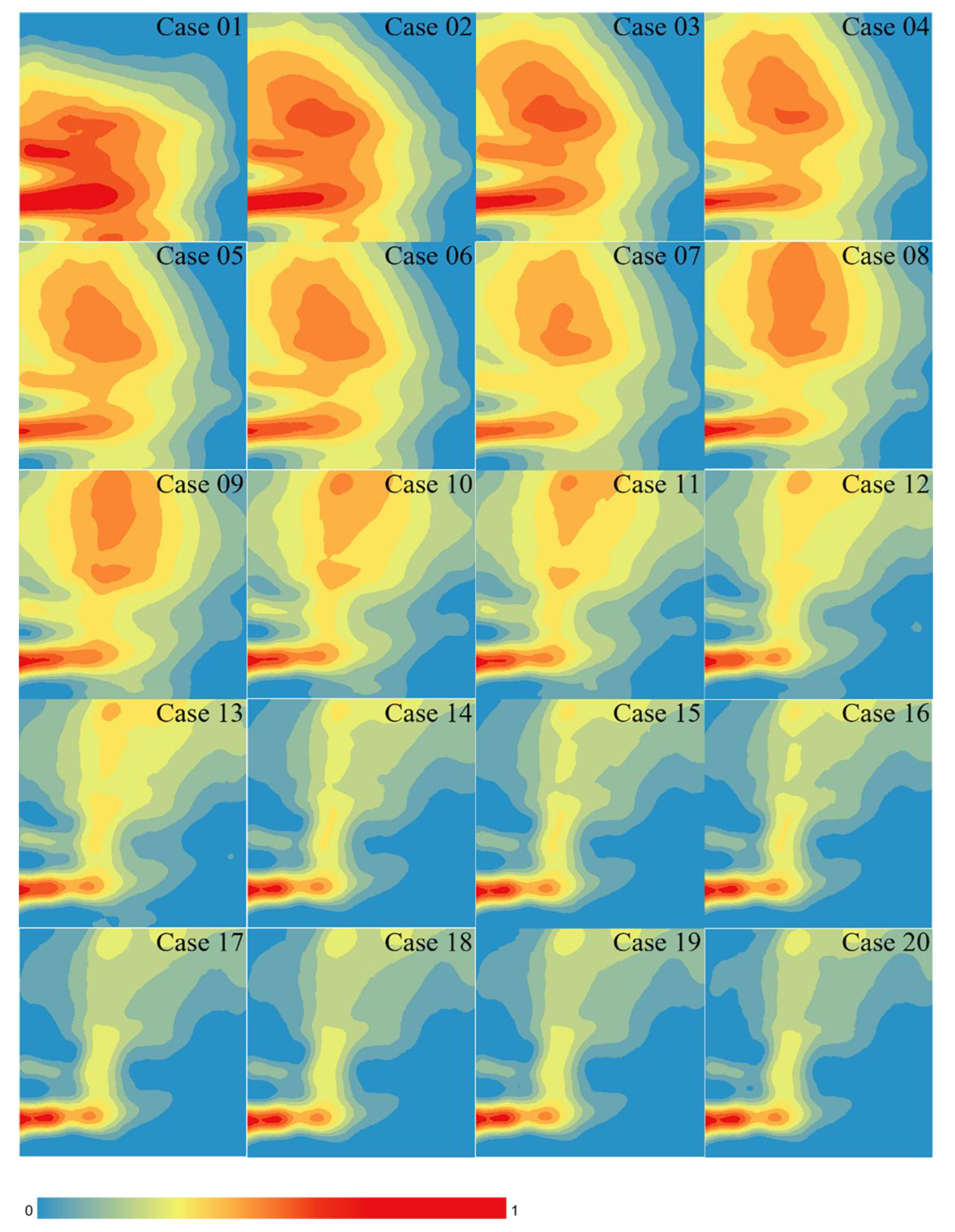
Figure 4 presents the normalized concentrations of diverse cases under the MGGP model. Fr, x, and y were chosen as input variables, and the normalized concentrations in diverse cases were predicted by the best model as the output variables. It can be observed from the figure that the prediction of the normalized concentration distribution of the MGGP model for diverse cases is consistent with the actual comparison, and the law of the concentration distribution changing with the Froude number is consistent with the actual data, but it is not difficult to see that the concentration distribution map obtained by the MGGP model has a large error: the occurrence of a higher concentration area above the port, which is inconsistent with the actual situation.
Figure 5 compares the prediction of the MGGP model with the normalized concentration of the actual data. From this figure, it can be observed that the prediction data are concentrated around the 1:1 line, so it can be judged that the performance of the MGGP joint method is basically good. The predicted values were compared to the actual values, and the RMSE and R2 values were calculated to further evaluate the model performance. It was calculated that the RMSE values of the training set and the test set were 0.087 and 0.088, and the R2 values were 0.903 and 0.902, respectively. The RMSE value was low and the R2 value was high, so the accuracy of the model prediction is acceptable, though large errors still exist.
When using the CNN method to train the model, the dataset division is improved, and the dataset is divided into training sets, validation sets, and test sets according to a 6:2:2 ratio. The training set is utilized to train the resulting neural network model, and then the validation set is utilized to verify the validity of the model, and the model that obtains the best results is selected until a satisfactory model is obtained. When the model “passes” the validation set, the test set is utilized to test the final effect of the model, and the accuracy of the model is evaluated by RSME, R2 value, and so on, including errors. The test set is only utilized for model testing, and it is absolutely impossible to adjust the network parameter configuration and select the trained model according to the results on the test set, otherwise the model will be overfitted on the test set.
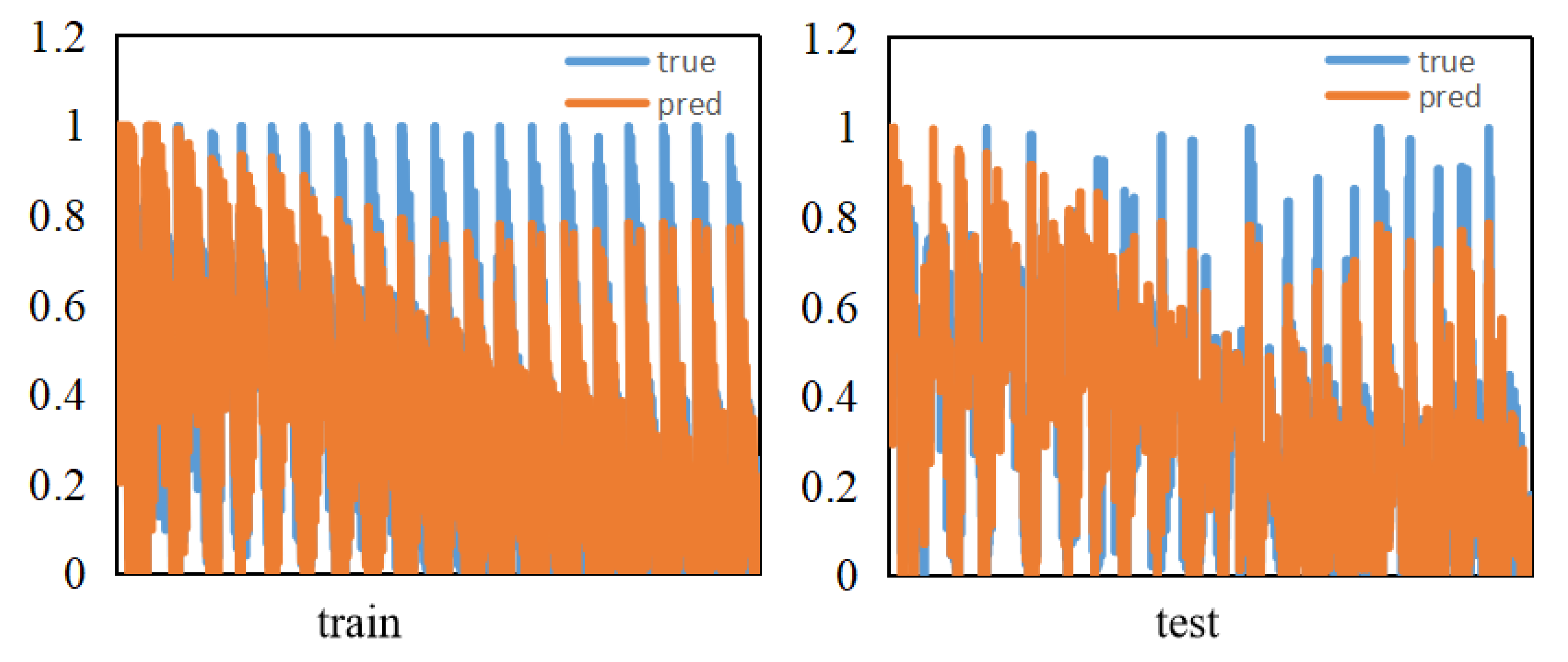
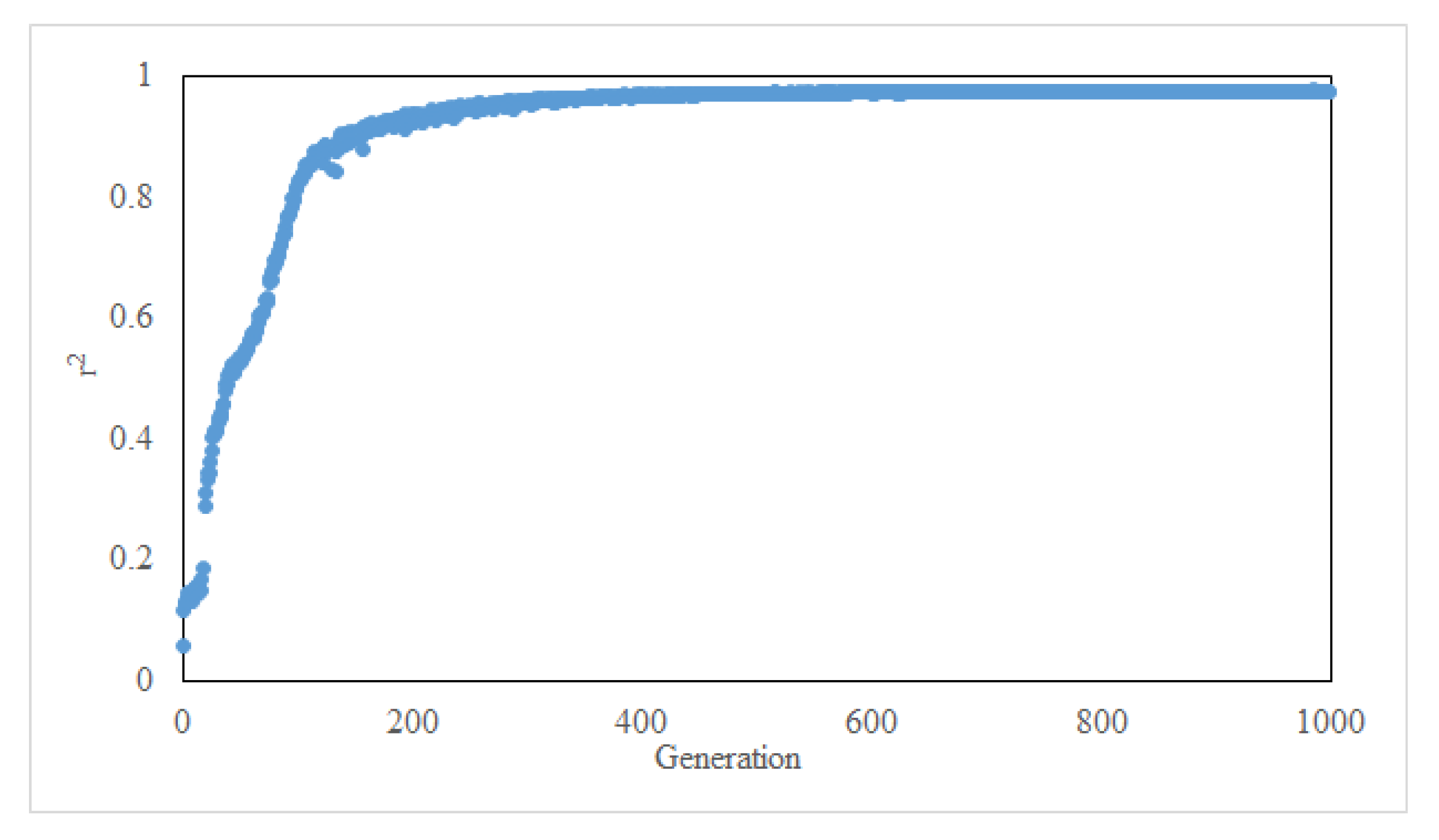
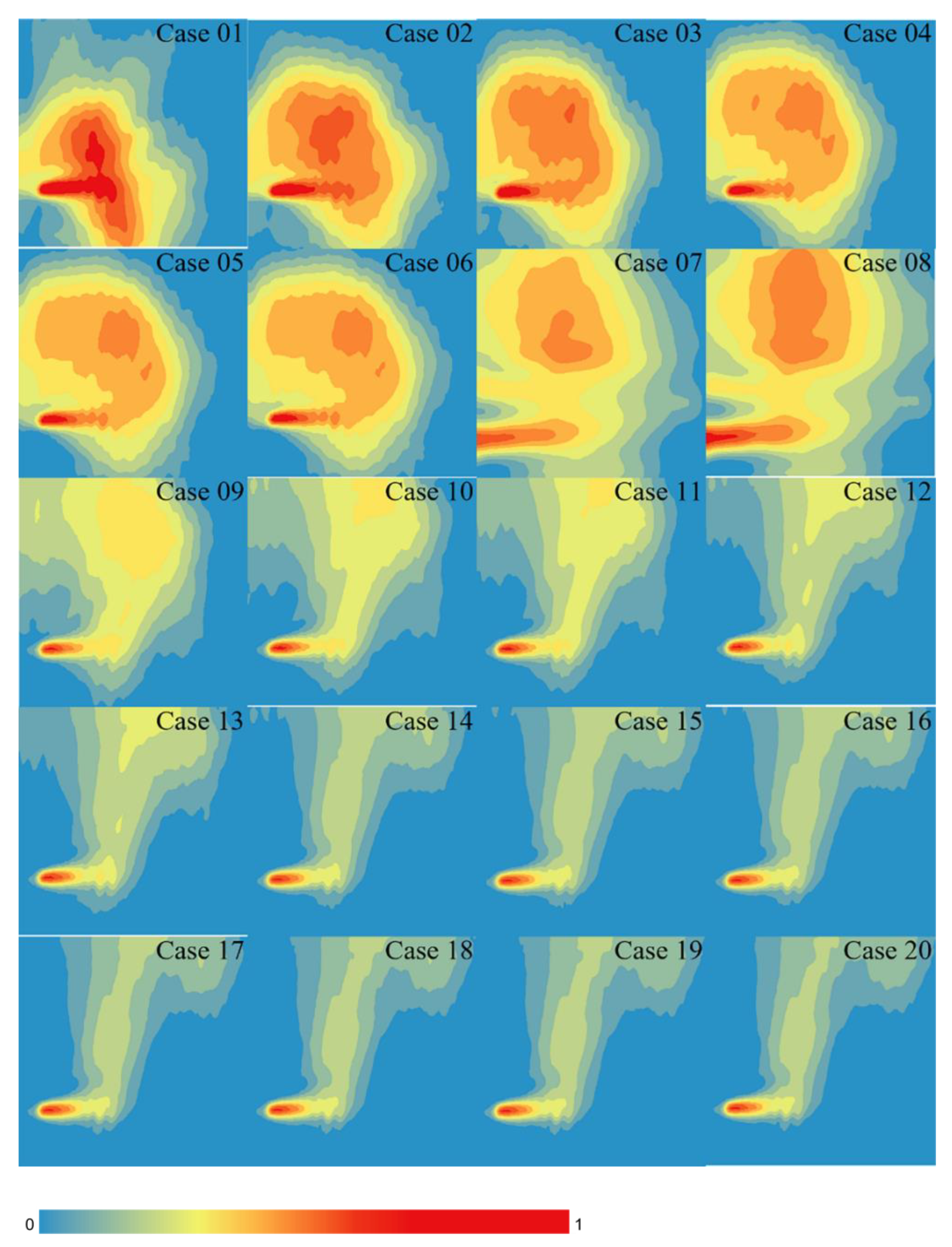
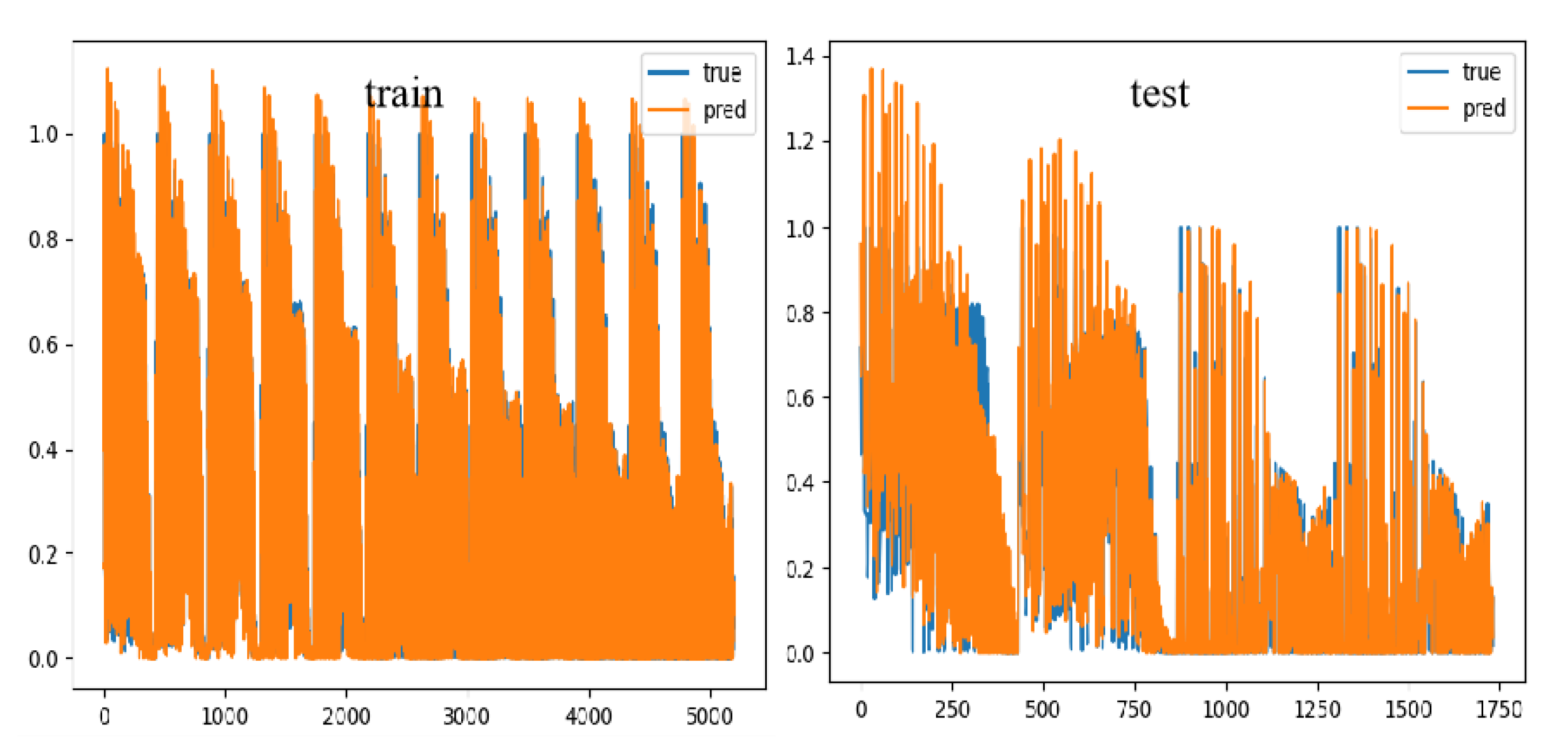
Figure 6 shows the adaptability of the CNN model at each evolutionary step. The CNN method also sets the training procedure to 1000 generations; the initial fitting effect of training is poor, with an increase in the number of changes, the R2 value is becoming larger and larger, the degree of fit is getting higher and higher, and after 300 generations, the result is not very diverse. According to the prediction of the normalized concentration of diverse cases at diverse locations, the normalized concentration field of the central plane is established, as shown in Figure 7. At large Fr values, the simulation prediction is not very good. This is due to the fact that the dataset is relatively small when Fr is larger, which also shows that machine learning requires a large amount of data for training in order to reduce errors. Overall, the prediction of the buoyant jet trajectory at the nozzle of the CNN method is highly consistent with the actual situation, showing an upward vertical jet. As can be observed from the figure, the CNN joint method predicts that the scope of sewage impact is basically consistent with the actual data, which provides a reference basis for determining the location of sewage diffusers and formulating environmental protection policies. In cases 1 to 8, the sewage has a large impact range and is round or elliptical. In cases 9 to 20, the boundary of the sewage impact range is more obvious, and it is greatly affected by buoyancy, which is consistent with the actual data obtained. The validation set is verified by using the trained model, and the resulting RSME value is 0.031 and the R2 value is 0.985, so it can be proved that the model passes the test and can be tested. The test set was evaluated using this model, and the resulting RSME value was 0.056 and R2 value was 0.956. Figure 8 compares the actual and predicted normalized concentrations of the CNN model. It can be observed from the figure that the CNN model prediction is consistent with the actual data trend, and the numerical size is not very diverse, so the prediction accuracy of the model is relatively high.
Compared with the models trained by the CNN and MGGP methods, the model obtained by the CNN joint method has a lower RMSE value and a higher R2 value, and the accuracy rate is significantly improved compared with MGGP. Compared with the normalized concentration distribution maps under diverse models, the concentration distribution maps obtained by MGGP have obvious concentration band fractures, and horizontal concentration distribution bands appear above the port, which is quite diverse from the actual concentration distribution. The concentration distribution map obtained by the CNN method is more consistent with the actual value, and the concentration band is basically the same, so it can be said that the simulation effect is better. The buoyancy jet trajectory was predicted by the CNN combined method, which was more consistent with the measured data, and the vertical normalized concentration distribution and diffusion range were basically consistent with the measured data. In addition, in terms of computing time, MGGP needs several hours to build a model, while CNN training time is relatively short and can be completed in a few minutes; therefore, the computational efficiency is greatly improved. This shows that the results of modeling predictions using the CNN method are superior to the MGGP method, which is an encouraging result in the domain of machine learning.

3.3. The Performance of the Proposed Approach

The CNN model has both reliability and the accuracy. From the perspective of spatial distribution, the CNN model can accurately capture the process of predicting the start, transmission, and diffusion of the buoyant jet. Quantitatively, the RMSE and R2 values calculated by the CNN model based on the buoyancy jet space coordinates are 0.056 and 0.956, respectively, which are higher than the 0.088 and 0.902 of the MGGP model, confirming that the CNN is greatly improved compared with other machine learning models. To the best of the authors’ knowledge, this is the first time a CNN model has been developed for jets or plumes. The CNN method has recently been employed in similar applications. For example, Syed Kabir et al. [32] developed a fast-prediction flood model based on the deep convolutional neural network method, which further confirmed the performance of the CNN model. We have shown that the CNN model greatly outperforms the SVR. Hossein Hosseiny et al. [33] proposed a general river flood modeling framework based on coupled hydraulics and ML modeling, and the results showed that machine learning can reduce the computational time, resources, and cost of large-scale real-time simulations with high accuracy. Compared with CNN technology, the R2 value of the CNN model in this study is 0.956; the R2 of Syed Kabir et al. using CNN modeling was 0.94, and the CNN model studied by Hossein Hosseiny et al. had an R2 of 0.88, which confirms that the accuracy achieved in this study is comparable to those achieved in previous similar studies. In the later research, more influencing factors will be added to continuously improve the accuracy of the model.

4. Conclusions

This research proposed a modeling of a rosette-type multi-port buoyancy jet based on a combination of CFD and CNN technologies. Using a validated CFD model to calculate 20 diverse Froude number cases, and then using CNN technology to build a machine learning model, the accuracy between the final prediction data and CFD physically based data is acceptable. The predicted data RSME value is 0.056 and R2 value is 0.956; when the Froude number is small, the buoyancy jet trajectory shows a significant upward parabolic shape, and the concentration distribution is consistent with the measured value. Compared with MGGP, the CNN model occupies less memory, the operation rate is faster, the accuracy of the results is higher, and the overall performance of the model is better. This study demonstrates the ability of this method in simulating the concentration field of a rosette buoyancy jet. When more data is available, the composite model can be further improved or the performance of the composite model can be extended. Furthermore, in machine learning, the training method and hyperparameter settings have a significant impact on the model training results, and in the training of neural networks, how to better train a model is a problem that is worth exploring.

Author Contributions

Conceptualization, X.Y. and Y.W.; methodology, X.Y. and Y.W. formal analysis, Y.W.; investigation, A.M.; writing—original draft preparation, Y.W.; writing—review and editing, A.M. and J.L.; visualization, Y.W. and X.C.; project administration, X.Y.; funding acquisition, X.Y. and A.M. All authors have read and agreed to the published version of the manuscript.

Funding

This research was funded by the Key Laboratory of Hydrometeorological Disaster Mechanism and Warning of Ministry of Water Resources, Nanjing University of Information Science & Technology, Nanjing, China [HYMED202206], the Fundamental Research Funds for the Central Universities (China; DUT20RC(3)096); the National Natural Science Foundation of China (Grant number 42077348), and Natural Sciences and Engineering Research Council of Canada (NSERC Discovery Grants).

Institutional Review Board Statement

Not applicable.

Informed Consent Statement

Not applicable.

Data Availability Statement

Not applicable.

Conflicts of Interest

The authors declare no conflict of interest.

References

  1. Yan, X.; Ghodoosipour, B.; Mohammadian, M. Three-dimensional numerical study of multiple vertical buoyant jets in stationary ambient water. J. Hydraul. Eng. 2020, 2020, 04020049. [Google Scholar] [CrossRef]
  2. Yan, X.; Mohammadian, A.; Chen, X. Three-dimensional numerical simulations of buoyant jets discharged from a rosette-type multiport diffuser. J. Mar. Sci. Eng. 2019, 7, 409. [Google Scholar] [CrossRef]
  3. Lai, A.C.; Lee, J.H. Dynamic interaction of multiple buoyant jets. J. Fluid Mech. 2012, 708, 539–575. [Google Scholar] [CrossRef]
  4. Abessi, O.; Roberts, P.J. Rosette Diffusers for Dense Effluents in Flowing Currents. J. Hydraul. Eng. 2017, 144, m06017024. [Google Scholar] [CrossRef]
  5. Abessi, O.; Roberts, P.J.; Gandhi, V. Rosette diffusers for dense effluents. J. Hydraul. Eng. 2016, 143, 06016029. [Google Scholar] [CrossRef]
  6. Yan, X.; Mohammadian, A. Numerical Modeling of Vertical Buoyant Jets Subjected to Lateral Confinement. J. Hydraul. Eng. 2017, 43, 04017016. [Google Scholar] [CrossRef]
  7. Zhang, S.; Law, A.W.K.; Jiang, M. Large eddy simulations of 45° and 60° inclined dense jets with bottom impact. J. Hydro-environ. Res. 2017, 15, 54–66. [Google Scholar] [CrossRef]
  8. Glaze, D.J.; Frankel, S.H. Stochastic inlet conditions for large-eddy simulation of a fully turbulent jet. Aiaa J. 2015, 41, 1064–1073. [Google Scholar] [CrossRef]
  9. Knystautas, R. The turbulent jet from a series of holes in line. Aeronaut. Q. 2016, 15, 1–28. [Google Scholar] [CrossRef]
  10. Yannopoulos, P.C.; Noutsopoulos, G.C. Interaction of vertical round turbulent buoyant jets—Part I: Entrainment restriction approach. J. Hydraul. Res. 2006, 44, 218–232. [Google Scholar] [CrossRef]
  11. Wang, H.J.; Davidson, M.J. Jet interaction in a still ambient fluid. J. Hydraul. Eng. 2003, 129, 349–357. [Google Scholar] [CrossRef]
  12. Yan, X.; Mohammadian, A. Multigene Genetic-Programming-Based Models for Initial Dilution of Laterally Confined Vertical Buoyant Jets. J. Mar. Sci. Eng. 2019, 7, 246. [Google Scholar] [CrossRef]
  13. Yan, X.; Mohammadian, A.; Khelifa, A. Modeling spatial distribution of flow depth in fluvial systems using a hybrid two-dimensional hydraulic-multigene genetic programming approach. J. Hydrol. 2021, 600, 126517. [Google Scholar] [CrossRef]
  14. Zhao, G.; Pang, B.; Xu, Z.; Peng, D.; Zuo, D. Urban flood susceptibility assessment based on convolutional neural networks. J. Hydrol. 2020, 590, 125235. [Google Scholar] [CrossRef]
  15. Mehr, A.D.; Nourani, V. A pareto-optimal moving average-multigene genetic programming model for rainfall-runoff modelling. Environ. Model. Softw. 2017, 92, 239–251. [Google Scholar] [CrossRef]
  16. Bayazidi, A.M.; Wang, G.G.; Bolandi, H.; Alavi, A.H.; Gandomi, A.H. Multigene genetic programming for estimation of elastic modulus of concrete. Math. Probl. Eng. 2014, 2014, 474289. [Google Scholar]
  17. Paiva, G.M.D.; Pimentel, S.P.; Alvarenga, B.P.; Marra, E.G.; Leva, S. Multiple site intraday solar irradiance forecasting by machine learning algorithms: Mggp and mlp neural networks. Energies 2020, 13, 3005. [Google Scholar] [CrossRef]
  18. Safari, M.J.S.; Mehr, A.D. Multigene genetic programming for sediment transport modeling in sewers for conditions of non-deposition with a bed deposit. Int. J. Sediment Res. 2018, 33, 46–54. [Google Scholar] [CrossRef]
  19. OpenFOAM User Guide; Version 4.0; The OpenCFD Foundation: London, UK, 2016.
  20. Yan, C.; Wang, C. Development and application of the convolutional neural network model. Comput. Sci. Explor. 2021, 15, 27–46. [Google Scholar]
  21. Wei, D.; Wang, B.; Zhang, M. Study on the Deep Learning Model of Concrete Dam Deformation Prediction Based on CNN. Water Conserv. Hydropower Technol. 2021, 52, 52–57. Available online: https://iopscience.iop.org/article/10.1088/1755-1315/580/1/012042/pdf (accessed on 14 September 2022). [CrossRef]
  22. Holzmann, T. Mathematics, Numerics, Derivations and OpenFOAM®; Holzmann CFD: Loeben, Germany, 2016. [Google Scholar]
  23. Eltner, A.; Bressan, P.O.; Akiyama, T.; Gonçalves, W.N.; Marcato Junior, J. Using deep learning for automatic water stage measurements. Water Resour. Res. 2021, 57, e2020WR027608. [Google Scholar] [CrossRef]
  24. Kreyenberg, P.J.; Bauser, H.H.; Roth, K. Velocity field estimation on density-driven solute transport with a convolutional neural network. Water Resour. Res. 2019, 55, 7275–7293. [Google Scholar] [CrossRef] [Green Version]
  25. Tian, C.; Xu, Y.; Zuo, W. Image denoising using deep CNN with batch renormalization. Neural Netw. Off. J. Int. Neural Netw. Soc. 2020, 121, 461–473. [Google Scholar] [CrossRef]
  26. Kiranyaz, S.; Ince, T.; Hamila, R.; Gabbouj, M. Convolutional Neural Networks for patient-specific ECG classification. In Proceedings of the 2015 37th Annual International Conference of the IEEE Engineering in Medicine and Biology Society (EMBC), Milan, Italy, 25–29 August 2015; pp. 2608–2611. [Google Scholar] [CrossRef]
  27. Zihlmann, M.; Perekrestenko, D.; Tschannen, M. Convolutional Recurrent Neural Networks for Electrocardiogram Classification. 2017. Available online: http://arxiv.org/abs/1710.06122 (accessed on 1 January 2022).
  28. Abdeljaber, O.; Avci, O.; Kiranyaz, M.S.; Boashash, B.; Sodano, H.; Inman, D.J. 1-D CNNs for structural damage detection: Verification on a structural health monitoring benchmark data. Neurocomputing 2018, 275, 1308–1317. [Google Scholar] [CrossRef]
  29. Sakhaei, Z.; Nikooee, E.; Riazi, M. A new formulation for non-equilibrium capillarity effect using multi-gene genetic programming (mggp): Accounting for fluid and porous media properties. Eng. Comput. 2022, 38, 1697–1709. [Google Scholar] [CrossRef]
  30. Searson, D.P. GPTIPS 2: An Open-Source Software Platform for Symbolic Data Mining. In Handbook of Genetic Programming Applications; Springer: Cham, Switzerland, 2015; pp. 551–573. [Google Scholar]
  31. Yan, X.; Wang, Y.; Mohammadian, A.; Liu, J. Simulations of the Concentration Fields of Rosette-Type Multiport Buoyant Discharges Using Combined CFD and Multigene Genetic Programming Techniques. J. Mar. Sci. Eng. 2021, 9, 1311. [Google Scholar] [CrossRef]
  32. Kabir, S.; Patidar, S.; Xia, X.; Liang, Q.; Neal, J.; Pender, G. A deep convolutional neural network model for rapid prediction of fluvial flood inundation. J. Hydrol. 2020, 590, 125481. [Google Scholar] [CrossRef]
  33. Hosseiny, H.; Nazari, F.; Smith, V.; Nataraj, C. A Framework for Modeling Flood Depth Using a Hybrid of Hydraulics and Machine Learning. Sci. Rep. 2020, 10, 8222. [Google Scholar] [CrossRef]
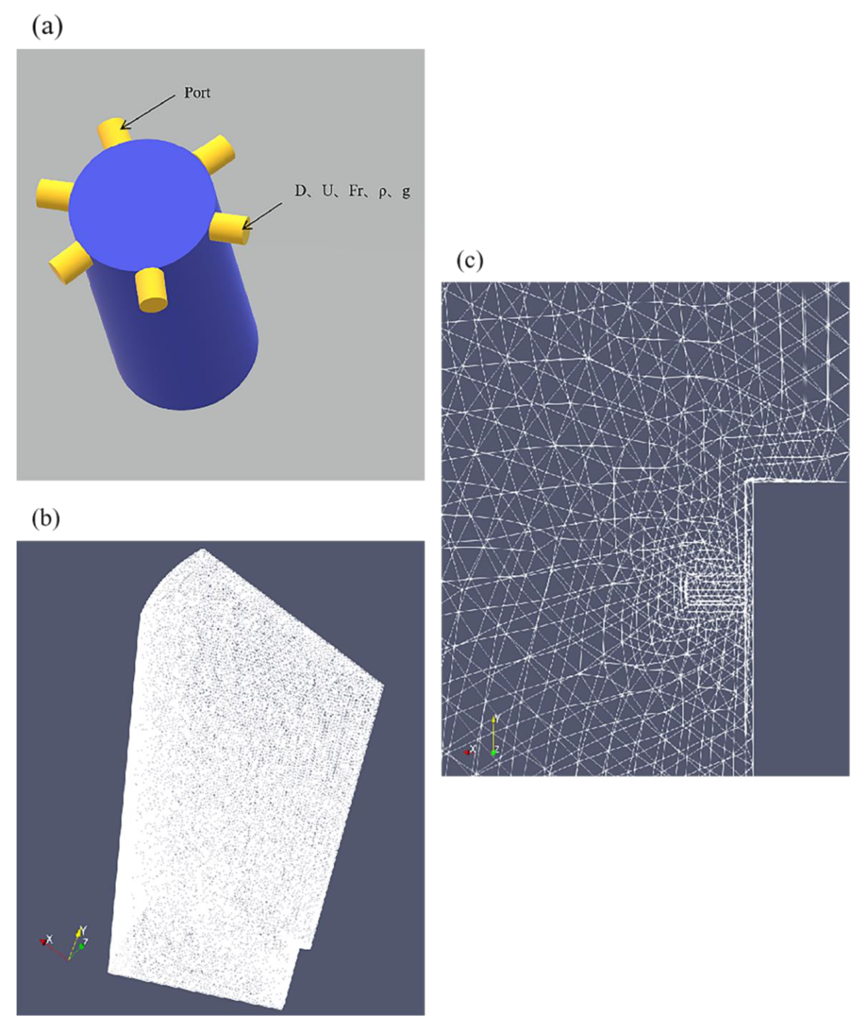
Figure 1. Rosette-type diffuser, computational domain, and mesh: ((a) shows a schematic of the diffuser, (b) is a computational grid, and (c) is a refined mesh near the discharge port).
Jmse 10 01383 g001
Figure 2. 20 cases of Froude parameters.
Jmse 10 01383 g002
Figure 3. The normalized concentration field of the central plane under different conditions obtained by CFD model.
Jmse 10 01383 g003
Figure 4. The normalized concentration field of the central plane under different conditions obtained by the MGGP model.
Jmse 10 01383 g004
Figure 5. Comparison of actual and predicted normalized concentrations.
Jmse 10 01383 g005
Figure 6. Fitness of CNN model in each evolutionary step.
Jmse 10 01383 g006
Figure 7. The normalized concentration fields on the central plane under different conditions obtained by the CNN model.
Jmse 10 01383 g007
Figure 8. Comparison of the actual and predicted normalized concentrations of the CNN model.
Jmse 10 01383 g008
Table 1. Model parameter.
DUFrρg
0.0044 m0.185 m/svariable997 km/m39.8
Table 2. Comparison of experimental results and simulation results.
y/Dx/D (Exp)x/D (Num)
0.401.280.99
1.762.562.84
3.123.523.67
4.883.924.39
37.724.485.13
6.574.644.80
8.014.965.10
35.484.965.09
9.695.285.35
33.155.285.20
11.135.525.53
30.755.525.32
28.115.685.47
25.715.765.64
13.535.845.79
19.145.846.23
20.985.846.19
22.745.846.02
15.225.925.99
17.0666.20
Publisher’s Note: MDPI stays neutral with regard to jurisdictional claims in published maps and institutional affiliations.