Abstract
Various models have recently been developed to describe Arctic coastal erosion. Current process-based models simulate multiple physical processes and combine them interactively to resemble the unique mechanism of Arctic coastal erosion. One limitation of such models is the difficulty of including hydrodynamic forces. The available coastal erosion models developed for warmer climates cannot be applied to Arctic coastal erosion, where permafrost is a significant environmental parameter. This paper explains a methodology that allows us to use the models designed for warmer climates to simulate Arctic coastal erosion. The open-source software XBeach is employed to simulate the waves, sediment transport and morphological changes. We developed different submodules for the processes unique to Arctic coasts, such as thawing–freezing, slumping, wave-cut niche, bluff failure, etc. The submodules are coupled with XBeach to enable concurrent simulation of the two mechanisms of Arctic coastal erosion, namely thermodenudation and thermoabrasion. Some of the model’s input parameters are calibrated using field measurements from the Arctic coast of Kara Sea, Russia. The model is then validated by another set of mutually exclusive field measurements under different morphological conditions from the study area. The sensitivity analysis of the model indicates that nearshore waves are an important driver of erosion, and the inclusion of nearshore hydrodynamics and sediment transport are essential for accurately modelling the erosion mechanism.
1. Introduction
Approximately one-third of the coast worldwide consists of permafrost, for which the average retreat rate is close to 0.5 m per year [1]. The annual retreat of the coastline along Alaska in the Beaufort Sea is 1.7 m per year [2]. In recent decades, the coastal retreat rate along the Kara Sea has been measured between 1 and 1.7 m per year [3]. The annual maximum retreats along the Alaskan coast were approximately 22 m for the years 2007, 2012 and 2016 [4,5,6]. Many other Arctic coasts are retreating at the same level of magnitude. The most significant erosion along the coast of the Kara Sea was observed to be 19.6 m in 2010–11 [7]. Observations along the various Arctic coasts have led to the establishment of a link between increased coastal erosion and a smaller extent of sea cover [8,9], warmer air temperature [10,11] and increased permafrost temperature [12].
The environmental changes due to warming of the climate are triggering significant coastal erosion in the Arctic [13]. The number of open-sea days in the Arctic is increasing rapidly [14]. The seawater temperature anomalies reached 5 °C in the Arctic Ocean [15]. The frequency and intensity of storms during summer are also expected to increase [16]. Increased thawing of permafrost inside the coastal bluffs leads to slumping and, consequently, loss of mass along the Arctic coast. On the other hand, the sea ice extent is shrinking, which enables longer fetches to generate larger waves [14]. A longer open sea season also increases erosion along the coast. As a result, Arctic coastal retreat has increased more than twofold in the last few decades [17,18,19,20].
Increased Arctic coastal erosion poses a significant threat to residents of coastal communities. Shoreline infrastructure is compromised, heritage sites are at risk, and the lifestyle of the indigenous people is also affected [20]. Moreover, within the next decade, the surface air temperature is expected to exceed the normal range of variability. In contrast, with regard to Arctic sea ice, the natural range of variability has already been exceeded [21]. A pan-Arctic model by Nielsen et al. [12] predicts that Arctic coastal erosion will exceed the natural variability range before the end of the century, with a 66% probability of exceeding by 2023 and over 90% probability of exceeding before 2049.
Are F [22] described two mechanisms that govern coastal bluff erosion in the Arctic: thermodenudation and thermoabrasion. In the thermodenudation process, thermal energy thaws the permafrost during the summer, leading to slumping of the thawed bluffs via gravitational forces. The slumped materials are removed from the beach by waves, tides and storm surges. Thermodenudation is a continuous process and contributes to the slow retreat of the coast. In contrast, thermoabrasion is rapid and episodic. Thermoabrasion is triggered during summer storms where surges inundate the beach, leading to the formation of a wave-cut niche at the bluff’s base. The growing niche becomes deep enough to trigger bluff collapse at one point. The collapsed bluff degrades on the beach and eventually washes away under hydrodynamic forcing.
There is still a limited understanding of the governing mechanisms behind Arctic coastal erosion. A fundamental element of the Arctic coasts, the presence of permafrost, creates a different condition compared to coastal erosion in a warmer climate. Permafrost acts as a slow-erodible structure when no thermal source is present. Along with thermal drivers, the mechanical component also contributes to erosion. Coastal erosion in the Arctic is sensitive to the presence of sea ice, which dampens the waves propagating towards the coast [23].
Several models have been developed to simulate Arctic coastal erosion over the past decade. Most of these models focus on bluff failure, where the growth of the niche is the central factor of the erosion mechanism. Such process-based models simulate wave-cut niche growth at the bluff base, destabilise the overhanging portion and lead to bluff failure. The earlier work of Kobayashi [24] provides the basis for most of these models. Kobayashi [24] developed an analytical solution of the inward growth rate of the niche as a function of the temperature of the incoming seawater, the depth of water at the base of the bluff and the duration of the inundation. Additionally, niche models developed for melting of icebergs via waves and currents [25,26] have also been used with modifications; for example, a factor for energy requirement ratio of pure ice and permafrost thawing [27]. Hoque and Pollard [28] modelled bluff failure as a loss of balance (moment failure) and shear failure (mechanical strength). A process-based model to connect niche growth and bluff collapse with hydrodynamic forcing was introduced by Ravens et al. [29]. They included oceanographic boundary conditions using 12-h time steps. Ravens et al. [29] coupled four physical processes as modules: storm surge, niche growth, collapse of the overhanging bluff over the niche and degradation of the collapsed bluff. Barnhart et al. [30] expanded the model of Ravens et al. [29] and incorporated the bluff stability concept of Hoque and Pollard [31]. Barnhart et al. [30] also employed smaller time steps (3 h) to capture erosion at higher temporal resolutions. To include the effect of morphological changes such as changes in the coastal profiles of the Arctic coasts, Ravens et al. [32] used the open-source software package XBeach [33] to simulate wave propagation, sediment transport, and slumping. The latter was achieved by modifying the avalanching module in XBeach originally developed for sandy dunes. Bull et al. [27] introduced finite element analysis to understand niche-induced bluff collapse in detail. Frederick et al. [34] developed the finite element model to obtain a detailed analysis of the formation of the niche and subsequent bluff collapse without assuming any predetermined failure planes Rolph et al. [35] developed a pan-Arctic level erosion model based on thermal energy balance on the beach, a model originally proposed by Kobayashi et al. [36].
Arctic coastal erosion is a combination of various physical processes. While detailed models of some of the processes exist, for example, the formation of a wave-cut niche during a storm [24,34], a long-term generic (not site-specific) comprehensive model has yet to be achieved [37]. The process-based numerical models developed for various sites usually simplify physics. More importantly, the interactions between processes in the models are either ignored or made one-way (the processes are consequential, following a strict order of precedence). The existing models are not generic to all Arctic coasts, specifically for beaches where erosion is a mix of thermodenudation (dominated by thermal processes) and thermoabrasion (mechanically driven).
This paper describes a comprehensive model that couples the thermodenudation and thermoabrasion processes with nearshore hydrodynamics and sediment transport. The waves and related hydrodynamic forcing, together with sediment transport and morphodynamics are simulated using XBeach. The in-house modules simulate the other dominant processes related to erosion. We adopt a modular approach for the numerical implementation where the submodules communicate at three-hour intervals. The model is calibrated and validated with field measurements from one of the Arctic coasts along the Kara Sea. The behaviour of the model and potential applications are demonstrated. The simulations show that the erosion mechanism is greatly influenced by nearshore hydrodynamics and provide justification for including a hydrodynamic model to simulate Arctic coastal erosion.
2. Model Description
This paper presents a comprehensive model to simulate thermodenudation and thermoabrasion simultaneously. The processes of thawing, slumping, niche growth, bluff collapse and collapsed-bluff degradation are coupled with the coastal erosion model XBeach. Two-way coupling is established between (1) hydrodynamic forcing and sediment transport in XBeach on the one hand and (2) mechanical and thermal erosion processes in the in-house model on the other hand.
2.1. Model Domain and Input Data
Arctic coastal erosion originates offshore with wave generation and increases in water level due to storms. Thus, the domain of our model begins offshore. Four boundaries divide the domain into three zones, i.e., offshore, nearshore and beach bluffs (Figure 1). The offshore zone of the domain is contained by boundaries BC1 and BC2. The boundary BC2 is defined where the mean sea level () and wavelength () bear a ratio of less than 0.5. The storm surge and wave generation in the offshore zone are simulated using a simplified 1D storm surge module [38] and SWAN [39], respectively. The SWAN and storm surge model are coupled with XBeach at the BC2 boundary. At the BC2, water level () and wave conditions (, , of JONSWAP spectrum) are specified based on SWAN and storm surge model results. The transformation of the wave, wave setup and set down, and morphological changes in the nearshore zone are simulated by XBeach. Permafrost-related processes thawing and erosion of the bluffs are simulated with in-house modules and coupled with XBeach.
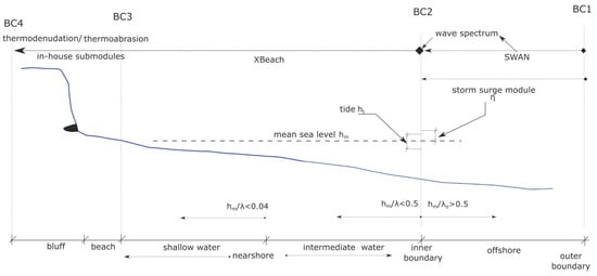
Figure 1.
The spatial zones of the model are marked with four boundaries. SWAN and storm surge modules calculate the hydrodynamics boundary conditions at BC2, which acts as input for XBeach. The outputs of XBeach are used as input for the submodules of thermodenudation and thermoabrasion.
Table 1 lists the parameters used to describe thermodenudation and thermoabrasion in our model. The geometric definitions are provided in Appendix A.

Table 1.
The list of main parameters used to describe the models.
2.2. Thermodenudation Module
The thermodenudation module simulates thermally driven processes within the beach and bluff. The processes of permafrost thawing and slumping at the bluff face are simulated using two submodules of permafrost thaw and slumping.
2.2.1. Submodule: Permafrost Thaw
We divide the permafrost thaw along the coastal profile into four sections, as shown in Figure 2. The warmer air and seawater bring the thermal energy necessary to thaw the permafrost inside the bluffs. The sections are defined based on the nature of the convective heat transfer. The four sections are the bluff surface, bluff face, beach and seabed (definitions are in Appendix B).
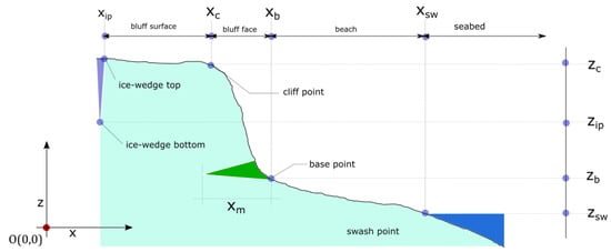
Figure 2.
The coastal profile can be divided into four sections based on the thermal energy transfer mechanism. The most active portion in terms of thawing is the bluff face.
The thawing depth () is defined as the depth of permafrost thawing or freezing face from the coastal profile, normal to each point, as shown in Figure 3. The thawing depth () is time-varying; it typically has the highest value in the summer and returns to zero during the winter. Stefan’s equation can be used to determine the thawing depth () [41]:
where t is the length of time (days), is the average dry density (kg m), is the specific latent heat of fusion (Jkg), w is the water content(%), and is the thermal conductivity of the unfrozen soil; a typical value of can be 1.6 JmsK and are the temperatures of the bluffs. However, Equation (1) overestimates the thawing and freezing depth [41]. The equation does not consider the fluid and surface interactions, air/water velocities, turbulence and geometric orientations. Equation (1) is not suitable for our model since we want to treat the dry and wet (submerged) parts of the coastal profile separately. We adopted another approach to estimate the thawing depth by calculating the heat transfer and subsequent thawing and freezing [32]. The energy transfer from the seawater or air to the sediment is estimated from the convective heat transfer equation:
where is the thermal energy transfer rate (energy per unit area per time) from water or air to the bluffs Jms, is the convective heat transfer coefficient (W/mk); different for air and water, is the temperature of the water or air, and is the temperature of the seabed and bluff.
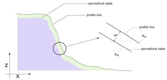
Figure 3.
The thawing depth is the distance normal to the permafrost to the surface of the bluffs ().
Assuming the temperature of the thawed layer remains close to the melting temperature and thus is responsible for the latent heat requirement of the phase change of permafrost, we can use Equation (2) together with Equation (3) to determine the thawing depth ():
where is the volumetric latent heat of fusion, taken as J/m3 [32], is the time duration in seconds and is the thawing depth assumed to be normal to the surface (see Figure 3).
The benefits of using Equation (3) over Equation (1) in our model are (1) the convective heat transfer coefficient can be calibrated to represent the different heat fluxes at bluff-surface, bluff-face, beach and seabed and (2) the equation is also valid for freezing when the fluid temperature drops below zero, allowing the submodule to remain active for all the seasons.
2.2.2. Submodule: Slumping
The failure of the thawed sediments by gravity as a layered movement or mudflow; without active contribution from waves is considered under the thermodenudation mechanism. Several slumping failure modes such as active layer detachment, solifluction, and retrogressive thaw slump are observed in the Arctic. In this paper, a simplified 1D model of mass movement is used in which we adopt a proxy parameter called critical slope (). The latter defines the threshold at which the thawed material will fall under the influence of gravity (see Figure 4). In general, the combined effect of sediment size distribution, ice content, consolidation status, internal friction and cohesion will determine the value of . The value of will vary for each coastal profile and must be carefully examined and calibrated. Further, we do not consider the effect of water flow inside the bluff nor the effects of sediment creep dynamics in our simplified slumping model. Moroever, we do not impose any upper limit on mass movement in our slumping model.
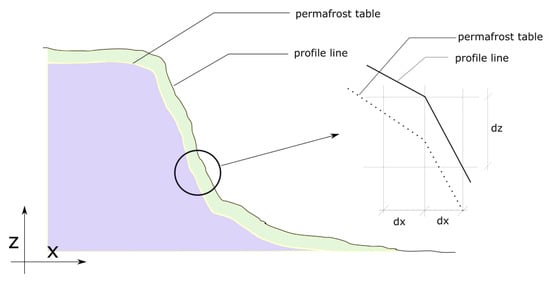
Figure 4.
Slumping occurs when the thawed materials fall due to gravity. The conditions for the triggering are: (1) thawing depth () is greater than zero and (2) slope at the point () is greater than the critical slope ().
The following conditions must be fulfilled to trigger slumping.
where is the slope of the coastal profile at a given point, and are the critical slopes for dry and wet conditions, respectively, and h is the time-averaged water depth. Some parts of the beach may temporarily go underwater by wave run-ups and the time-averaged water depth (in our model three hours) will have a small positive value at some of the grid points even though the heat is exchanged from the warm air. To overcome this problem, an arbitrary small threshold value of 0.05 m is chosen. When the water depth m, we consider the portion of the profile submerged. The assumptions related to slumping and numerical implementation are discussed in detail in Appendix C.2 and a standalone example of the slumping module is available in the Supplementary section.
2.3. Thermoabrasion Module
During storm surges with a combined effect of waves (wave setup, wave run-up) and tide, the water reaches the base of the bluffs, and a niche starts to grow. This module simulates the niche growth, subsequent bluff collapse, and collapsed-bluff degradation as three submodules. The behaviour of the submodules is highly dependent on the boundary conditions at the base of the bluffs, especially the water level at the base of the bluffs () and water temperature ().
2.3.1. Submodule: Niche Growth
When the water level reaches the base of the bluff (point B in Figure 5), the warm water creates a niche. The geometry depicted in Figure 5 is adapted and simplified from the Kobayashi [24] model.
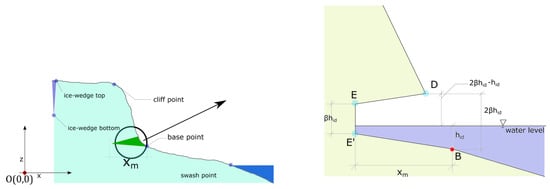
Figure 5.
Niche geometry during the storm surge; simplified from Kobayashi (1985).
The water depth at the base of the bluff; point B in the figure termed is obtained from the results of the XBeach simulation. The thawing face, line EE′, is vertical and assumed to be , where is the empirical parameter. The value of is taken as 2 [29]. The niche depth, line BE′ = , is estimated from the equation:
where is the time-averaged depth of water at the base of the bluff (m), g is the gravitational acceleration (m/s2), is the surf zone diffusivity , A is an empirical constant, taken as 0.4 [42], , is the temperature of the seawater and is the salinity adjusted melting point of the ice.
2.3.2. Submodule: Bluff Collapse
The wave-cut niche at the base of the bluff creates instability, which may lead to bluff collapse. A critical combination of the various geometric parameters, such as niche opening, niche depth, position of the ice-wedge polygon and mechanical strength parameters, such as internal friction and cohesive strength, leads to the collapse of the bluffs. The location of the failure line and plane may vary depending on the combinations of the various parameters. Two principal modes are identified for bluff collapse: (1) shear failure and (2) overturning failure [31]. Shear failures are related to the mechanical strength of the bluffs. In Figure 6, one of the three shear failure modes is depicted (the modes are discussed in Appendix C.3). The shaded region over the niche is susceptible to collapse. The failure line, in this case, is GE, and the shaded region by the geometry GCDE is collapsed. A generalised and simplified condition of shear failure of the bluff is Equation (6) [28]:
where is the angle of inclination of the failure plane, is the angle of internal friction of the bluffs, is the tensile failure line of the bluff (m), c is the tensile strength of the bluff (N/m), and W is the weight of the collapsed bluff (N) (weight of the GCDE portion in Figure 6a).
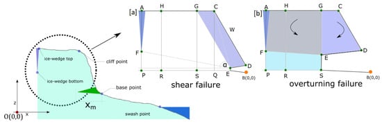
In the overturning failure mode, the failure is initiated by the moment created by the overhanging portion of the bluff. The overturning occurs at the thawing face of the niche at point E in Figure 6b. The shaded overhanging portion (GCDE) creates the driving moment in favour of collapse, which is countered by the moment created by the remaining portion of the bluff (AHGEF). A small contribution comes from the friction along failure line EF and line AF. The failure mode is generalised by the following Equation (simplified from the models by Hoque and Pollard [28] and Barnhart et al. [30]):
where is the moment created by the overhanging bluff at the turning point (N-m), is the opposite moment created by the rest of the bluff (N-m), c is the cohesive strength of the bluff (N/m2) (different for ice and permafrost), is the horizontal failure line (line FE in Figure 6), and is the vertical failure (line AF).
2.3.3. Submodule: Degradation of Collapsed Bluffs
The collapsed bluff remains on the beach and degrades over time. The degradation rate of the bluff can be estimated from the following Equation [29]:
where is the mass of the collapsed bluff at the end of timestep i, is the mass of the bluff at the end of the previous timestep , is the seawater temperature, is the salinity adjusted melting point of ice, H is the significant wave height at the 3-m water depth, and a and n are the empirical parameters. Ravens et al. [29] estimated that the values of a and n are 800 kg/m−°C and 1.47, respectively. In the numerical implementation of bluff degradation, we assume an immediate degradation of the collapsed bluff and the sediments are distributed evenly on the beach. The coupled hydrodynamic module simulates the removal of sediments from the beach.
2.4. Numerical Implementation
2.4.1. Hydrodynamics of the Offshore
Wave conditions and the water level are determined at the BC2 boundary as shown in Figure 1. SWAN determines the wave generation in the domain contained by the boundaries BC1 to BC2. A one-dimensional (1D) storm surge model calculates the storm surge () at the BC2 boundary. Numerical implementation of the storm surge model is detailed in Appendix C.1. The storm surge model is a function of wind speed, alongshore current, pressure drop, and the Coriolis effect.
2.4.2. Hydrodynamics of the Nearshore
We choose XBeach to simulate hydrodynamics, sediment transport and morphological changes from BC2 (in Figure 1) until bluffs. The input parameters at the XBeach offshore boundary at BC2 are time series of JONSWAP spectrum for waves, tide, mean sea level, storm surge, etc. A complete list of the XBeach parameters is provided in the Appendix F. XBeach simulates the wave transformation, wave set up and set down, run up, water level, tide and morphological changes in the nearshore zone. The results of the XBeach simulation are fed into the in-house submodules of thermodenudation and thermoabrasion. The timestep for the global model is chosen to be 3 h (Figure 7). The choice of global timestep is made by following the common practice in wave modelling and is consistent with most of the available metocean databases where stationarity is usually assumed over a period of 3 h and thus the sea state within the timestep is described with a spectrum. We simulate the hydrodynamic forcing and sediment transport of nearshore with XBeach for the i-th timestep and analyse the results. We determine the bed level changes, average water depth at the base of the bluffs (), and the mean water depth at each grid (to determine the wet/dry condition for convective heat transfer). The output of XBeach is then fed into the submodules of slumping, thawing depth, niche growth, and bluff collapse.
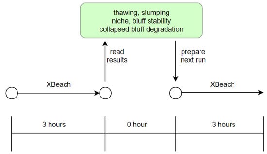
Figure 7.
XBeach simulates the nearshore module. The XBeach output is analysed and used as inputs for other submodules.
2.4.3. Modelling Permafrost and Thawing Depth
The permafrost and the thawed layer above the permafrost need to be treated separately to simulate thermodenudation. The thawing submodule calculates the thawing depth at the interval of each time step. The thawed layer above the permafrost reacts to hydrodynamic forcing similar to a typical coastal profile in a tropical or subtropical climate. Within XBeach, the ‘nonerodible’ surface layer feature aims to treat the effect of hard structure on the morphological changes in the coastal profile. The ‘nonerodible’ features allow users to include a surface that is unaffected by hydrodynamic forcing, and sediment transport is not permitted even if this surface is exposed. The ‘nonerodible’ surface can be defined with , and the user can place it inside the dune, beach and seabed. The permafrost acts similarly to a nonerodible surface, only that the permafrost line is a moving boundary with respect to time. In the numerical model, we achieve it by updating the of XBeach from the thawing depth () estimated at the end of the time step.
2.4.4. Workflow of the Numerical Model
A few threshold values are pre-set in the model. First, we adopt a threshold value of 20% for ice concentration below which the effects of sea ice on waves are neglected and above which waves are assumed totally attenuated before reaching the coast. This choice of threshold value provided a good fit with the field measurement, and is also similar to the threshold values adopted by Rolph et al. [35] and Overeem et al. [14]. Further, we adopt a threshold value of 5 cm to the time-averaged water depth in the cell; below this threshold, the cell is considered dry. We should recall that the time-averaged water depth (in our model over a period of three hours) will attain a small positive value if the cell is submerged only for a small portion of the timestep. If this positive value is very small, we expect that the dominant heat exchange mechanism will be convective heat transfer from the warmer air and thus the cell is to be considered fully dry. The choice of the threshold value is optimised to assure model stability (i.e., we seek the smallest possible value without compromising the stability of the model). A value of 5 cm is considered appropriate. Finally, we adopt a threshold value of 10 cm to the time-averaged water depth at the base of the bluff (); below this threshold, the niche module will not be activated. The choice of this value is also optimised to assure model stability similar to the above.
As discussed earlier, the morphological changes and wave transformations are simulated using XBeach. The workflow of the submodules is shown in Figure 8. At the inception of the simulation, global parameters such as the volumetric latent heat of permafrost thawing (), the tensile strength of bluffs (), geometric parameters such as and for air and water, etc., are loaded. These parameters are time-independent, i.e., remain the same for all timesteps. The input parameters, such as air temperature (), water temperature (), ice concentration (), wind speed (), bluff temperature (), and tide () are dependent on time. The model requires the time series of these input parameters at the same time interval as the global timestep. We set the global timestep as 3 h to be consistent with the three-hour sea-state and wave spectrum.
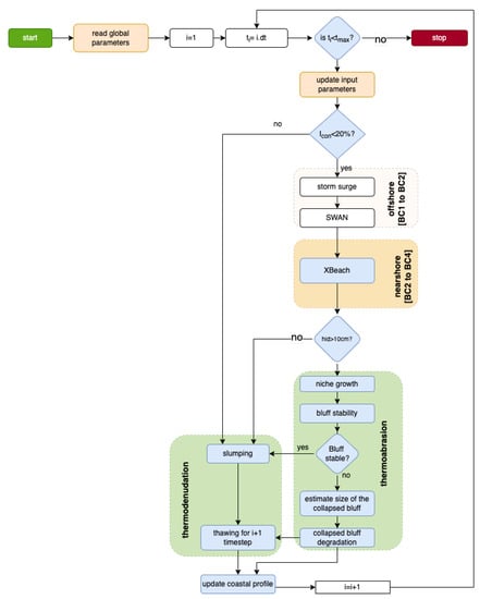
Figure 8.
Numerical implementation workflow of the submodules.
At the beginning of the i-th timestep, we must check whether the current timestep is within the simulation duration. If the condition is satisfied, we load the input parameters from the respective time series for the i-th timestep. The numerical model checks the ice concentration () for the current time step. From here, it is possible to proceed following two different routes. The offshore wave generation and storm surge is calculated only if the ice concentration is less than 20%. If the ice concentration is more than 20%, then the numerical model does not run SWAN, storm surge model and XBeach. We skip to the slumping submodule. An ice concentration of more than 20% indicates no wave activity. However, thawing and slumping might still occur even without hydrodynamic forcing. The numerical model activates the slumping submodule to accommodate this condition. The slumped sediments are moved to the bluff base. Since no hydrodynamic forcing is present in this route, the deposits at the base will not be transferred, and the model allows the accumulation of slumped sediments over the time steps. The accumulated sediments may be transported later when XBeach is activated.
Another route in the workflow is triggered when the ice concentration is less than 20%. If this condition is satisfied, then SWAN and storm surge submodule are turned on. The storm surge water level () and wave spectrum are calculated at boundary BC2. The water level is updated at BC2 for the tide and storm surge.
The XBeach simulates sediment transport, currents, water level setup, and morphological changes. The niche submodule becomes activated when the water level at the bluff () reaches more than 10 cm. We also calculate the time-averaged water depth at every grid point to determine whether the coastal profile is wet or dry at the i-th time step. The dry and wet grid points of the coastal profile are treated differently with respect to convective heat transfer and slumping (Equation (3)).
The model enters the thermodenudation module if the is less than 10 cm (which means the sea is calm, it is a ‘no storm’ condition), the slumping submodule is turned on. If is greater than 10 cm the model enters to thermoabrasion module and the niche submodule is activated. It calculates the growth of the niche (). The niche geometry is fed into the bluff stability submodule to check whether a collapse is triggered. The model returns on the thawing depth submodule when no bluff failure is recorded. When the model registers a bluff failure, it estimates the collapsed bluff’s size and volume, and the collapsed bluff degradation module is activated. After that, we calculate the thawing depth at each grid point for the i + 1 th time step. The last step of the model run at the i-th time step is registering the changes and updating the coastal profile to simulate the i + 1 th iteration.
The model described in this section is generic and thus applicable to most unlithified Arctic coasts for all seasons. Both thermodenudation and thermoabrasion can be simulated simultaneously. In the upcoming sections, we demonstrate in detail the application of the numerical model. Available field observations from one of the Arctic coasts in the Kara Sea were used to first calibrate the model, and the subsequent validation was performed using another set of field observations from different years of the same coasts.
3. Field Observations
Field investigations on one of the Arctic coasts, Baydaratskya Bay in the Kara Sea, have been conducted since the summer of 2012. The study area is in the north-east region of Russia (68.853096 N; 66.891730 E). The coast is situated in the gulf between the Ural coast and the Yamal Peninsula (see Figure 9a). The region is not densely populated, there is limited infrastructure and few indigenous settlements are present. The harsh climate and lack of communication facilities hinder continuous access to the study area. Lomonosov Moscow State University (MSU), under the project Centre for Research-based Innovation (CRI): Sustainable Arctic Marine and Coastal Technology (SAMCoT), investigate the study area during summer (between June and September) when it is accessible by road. The importance of studying the area increased after the Nord Stream gas pipeline was constructed in 2011 [43]. The results obtained from the field observations, measurements, and in situ experiments form the basis of this study.
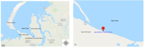
Figure 9.
[a] The study area is situated in the Kara Sea between the shallow gulf of two peninsulas, Yugra and Yamal. Image source: Google Maps. [b] The Arctic beach is straight and consists of continuous permafrost; the shore-normal line creates a 73 line to the north. Image source: Google Maps.
3.1. Morphological Description
The study area can be divided into two primary observation sites, S#1 and S#2 (see Figure 10). S#1 consists of low-lying bluffs ranging between 3–5 m, whereas S#2 comprises 12–15 m of high terraces. S#1 is approximately 1.2 km long. The bluff surface is smoothly sloped. A leida (low-lying land at the coast which is flooded during summer by storm surges) with a shoreline spanning 1.4 km lies between the two sites of S#1 and S#2. The Leida zone has an elevation above the tide level. Only surges created by storms in the summer can flood the leida. The surface run-off created many gullies on the surface of the area in S#1. Regarding sediment, both sites consist of silty clay, silt and silty sand. The permafrost in the study area is continuous; the annual mean temperature at a depth of 3 m is −4 Celsius [3]. The active organic layer measures approximately 0.5–0.8 m at the surface.
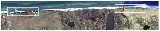
Figure 10.
The study area consists of two sites, S#1 and S#2, with distinct bluff height differences. S#1 consists of low bluff heights. Coastal profiles are shown with red lines. Image source: Internal reports, SAMCoT.
3.2. Data and Methods
3.2.1. Coastal Profiles
The coastal profiles of the study area are surveyed using the Differential Global Positioning System (DGPS). Geo-referencing is completed using handheld DGPS receivers and employing some stable objects to identify the profile in the field. After that, the observations are linked to the Russian State Geodetic Coordinate System (GSK-2011). Coastal features such as bluffs and shorelines are recorded. In 2018, surveying via light detection and ranging (LiDAR) began. Figure 11 shows one profile from each site.
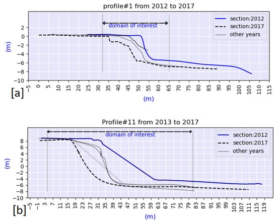
Figure 11.
Measurements of two coastal profiles in S#1 and S#2 are shown. [a] Measurements of profile P#1 in the zone S#1. [b] Measurement of profile P#11 in zone S#2. The bluff height in this profile is approximately 14 m.
Profile#1 in S#1 has a bluff height of 5–6 m. The profiles were covered with snow during measurements taken in 2013, 2014 and 2015. In 2017, we distinctly noticed the collapse of the bluffs near the cliff. Profile#11 from S#2 has a similar cliff retreat magnitude. Unlike Profile#1, the slope of Profile#11 remains constant over the years.
3.2.2. Nearshore Marine Observations
The seabed slope in the study area is 0.004 to 0.01 in the nearshore [44,45]. The length of the open seawater season has been increasing in recent years. From 1979 to 2006, the open sea days increased by 34 days [46]. The salinity of the seawater ranges from 20–25 ppt [47]. The tidal range near the shore is 70 cm, and the tidal currents do not exceed 30 cm/s [48].
3.2.3. Permafrost and Soil Temperature
As part of the investigations, boreholes are constructed at the study sites. Thermistors are used to measure the temperature at 12-h intervals. The boreholes are approximately 3.5 to 9 m deep. From the measurements, we observed that at the bluff’s base, the temperature does not fluctuate and remains stable between −5 to 0 Celsius.
3.3. Permafrost and Soil Properties
The dry density () of the sediments from the bluff is measured to be 2630 kg/m. The particle distribution of the study area is shown in Table A1. The ice content of the bluff ranges between 15–25% [49]. During the summer, the water content of the thawed permafrost was measured to be 29% [3]. About 60% of the sediment on the beach is within the range of 0.25–0.50 mm [3].
3.4. Erosion Pattern in the Study Area
We observed that both thermoabrasion and thermodenudation are active in the study area. During the summer, the thawing is continuous, and slumped materials accumulate on the beach. Figure 12 depicts the wave-cut niche at the base of the bluff at profile#11. The niche has not reached a critical length where the overhanging bluff is destabilised. The vertical position of the niche is higher than that at high tide. It was formed by a storm surge before the observation was made. During observation, no loose sediment was noticed at the base or inside the niche opening. The return currents must have carried away the sediments when the storm flooded the beach.
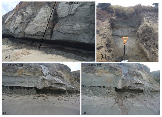
Figure 12.
[a] Status of Profile#11 during the 2015 measurement. The coastal profile#11 is shown as a black line. A wave-cut niche is visible at the base of the bluffs. Image source: SAMCoT Report, 2015. [b] Permafrost inside the bluff was excavated during the field investigation in 2015. Image source: Gorshkov, SAMCoT Report 2015, [c,d] six-hour time-lapse of thermodenudation in S#1. Niche is visible at the base of the bluffs, but the bluffs are stable. Accumulation of slumped sediments at the base. Image source: Vladislav Isaev. SAMCoT Report, 2015.
The permafrost layer inside the bluffs during summer is shown in Figure 12b. The thawed layer above the permafrost is approximately 0.5 to 1 m at the bluff surface. It is clear from the figure that the thawed layer has a considerable thickness at the bluff slope. We can infer that the intensity of the slumping (mass flux) is the limiting process for thermodenudation. In other words, the thawing rate () can be higher than the reduction rate of the thawed layer () due to slumping.
The following summarises the observations in general:
- Thermodenudation at the bluff face may be active, even when sea ice is present, and land-fast ice remains at the base of the bluffs. Unlike thermoabrasion, the open water season is not a prerequisite for thermodenudation.
- Thawed sediments from the bluffs fall under gravity and expose the permafrost underneath. The slumped materials are loose and accumulate on the beach.
- Wave-cut niches are developed at the base of the bluffs, while the bluffs may still be stable. Several storms may elongate the niche depth to a critical depth. Unless the niche depth reaches the critical length, the bluff remains stable.
- Thawed sediments accumulated at the base of the bluffs remain there until an extreme event creates a higher water level and return current.
4. Calibration of the Model
Some of the model input parameters, such as critical slope (), convective heat transfer coefficient (), water level (), and tensile strength of permafrost (c) are usually site-specific. In this section, we attempt to calibrate these parameters against field measurements from zone S#1 and S#2 of the study area. One profile from each zone (P#1 in S#1 and P#8 in S#2) are used. These two profiles are considered mutually exclusive because the profiles are different in geometry (bluff height and bluff slope) and geological settings. We treat each profile as a separate case and expect different calibrated parameters. However, the mean sea level is kept the same for both cases.
4.1. Methodology of Calibration
The convective heat transfer coefficient of the permafrost thaw module is calibrated against measurements of the thawing depth (). The thawing depth at the bluff surface is estimated from the temperature measurements at S#1. A thermistor string is installed in the borehole drilled on the bluff surface, 14.07 m from the crest of profile#3 (see Appendix E). Temperature measurements are taken at 12-h intervals along 20 nodes until reaching a depth of 2.43 m.
We do not have enough measurements to estimate uncertainties in the model input parameters, e.g., to fit a probability density function for each parameter. Hence, we used an upper- and lower-limit value for each parameter. These limits were deducted based on a theoretical evaluation or from field observations. Once the limits were identified, a trial-and-error procedure was used to calibrate some of the parameters. It should be mentioned that the available measurements were collected during testing campaigns conducted near the end of the summers of 2015 and 2016 (in mid-September, three to four weeks before winter started). The erosion measurements do not distinguish thermodenudation from thermoabrasion erosion. Therefore, we could only execute the calibration herein by running a one-year simulation (from 15.09.2015 to 14.09.2016) with different combinations of input parameters and selecting the combination that yields the minimum difference between the simulated and measured total erosion volume.
The morphological changes in the coastal profile from the shoreline to the bluffs are considered for calibration. The calibration process intends to simulate the morphological changes at the bluffs and the beaches as close as possible to the measurements. The indicators of erosion measurements, such as (a) crest retreat, (b) erosion volume, and (c) slope of the bluff face, are the targets. Out of the three erosion indicators, the primary aim is to simulate erosion by volume, i.e., the volumetric changes between the two measurements of consecutive years with minimum deviation from measurements. We measure erosion as volume changes spanning from the shoreline up to 15 m from the cliff towards the land. The erosion measurement is the volume per metre along the shore parallel line: (mm−width). The following equation is used to determine the erosion volume (Figure 13):
where E is the erosion volume, n is the grid point at the shoreline, N is the grid point 15 m from the cliff point, is the horizontal distance between two grid points, a is the measurement of the previous year and b is the measurement of the current year. A positive E value represents erosion, whereas negative values indicate accretion. We used ‘net erosion’ to describe the arithmetic sum of erosion and accretion.
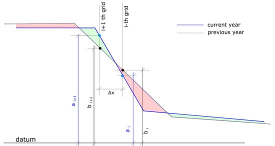
Figure 13.
A schematic of erosion volume calculation where a and b are the previous and current measurements from n to N grid points. The datum can be any arbitrary level since we are measuring differences. Positive erosion volume (E) indicates erosion.
We use root mean squared error (RMSE) to measure the performance of the calibration. The equation to calculate the RMSE values is as follows:
where RMSE is the root mean squared error, i is the variable, N is the number of grid points of simulation and observation, o is the observed value at the grid point and is the simulated value at the grid point.
4.2. Calibration of the Convective Heat Transfer Coefficient for the Bluff Surface
A continuous time series of thawing depth for the summer of 2017 is established by interpolation of the temperature measurements from borehole#4 on profile#3 (shown in Figure A5 in Appendix E). The thawing depth () during the summer of 2017 is simulated by applying the permafrost thaw module and compared with the measurement (Figure 14a). Different values are used with several iterations to seek the optimum value of that ensures the lowest RMSE when compared with the thawing depth measurements (Figure 14b).
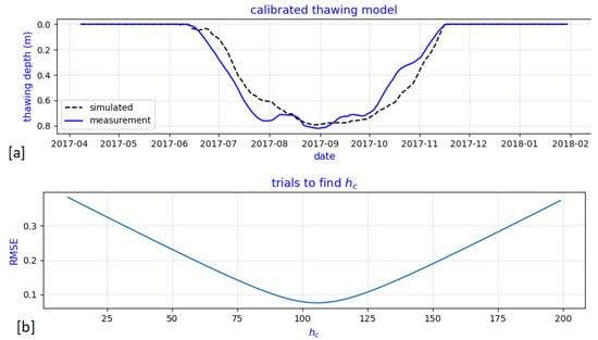
Figure 14.
The thawing depth measurement and simulation by the thawing module are shown in sub-figure [a]. The convective heat transfer coefficient () is iterated to minimize the RMSE error (sub-figure [b]). The lowest RMSE error is 0.1m for value of 106 for the bluff surface.
4.3. Calibration of Remaining Parameters
We choose two cases as described in Table 2 for the calibration. The case studies are termed case#1 and case#2. Both cases are from the same period. The coastal profiles of case#1 and case#2 are shown in Figure 15 and Figure 16, respectively.
Table 2.
A summary of the cases for calibration.
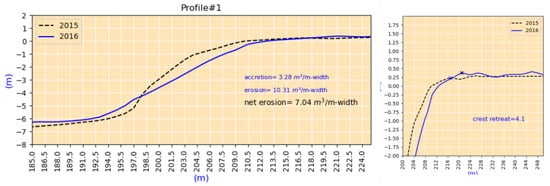
Figure 15.
The coastal profiles of case #1, from 2015 to 2016.
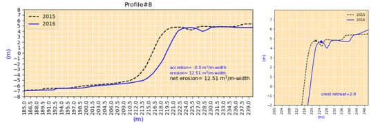
Figure 16.
The coastal profiles of case #2, from 2015 to 2016.
The cases started in September 2015 and ended in September 2016. We make the following observations about the cases:
- 1.
- The bluff height for case#1 is 6 m, and for case#2 is 13 m. The bluff slope of case#1 is approximately 0.4, which is lower than the bluff slope of case#2 (0.9).
- 2.
- The cases demonstrate different erosion patterns. For case#1, we note that the profile has undergone both erosion and accretion; the value of erosion is almost three times the accretion value (Figure 15). The accretion value indicates that the sediments accumulated in the lower part of the bluffs. No accretion is measured for cases#2 (Figure 16). For case#2, all the sediment from the erosion must have been washed away offshore.
- 3.
- The crest retreat for case#1 is 4.1, which is larger than that of case#2, even though the erosion volume of case#1 is lower. Because of the higher bluff heights (13 m vs. 6 m) for a similar crest retreat, case#2 had higher erosion volume.
- 4.
- The changes in the bluff slope are negligible for case#2 but significant for case#1. For case#1, the bluff base did not retreat; instead, the crest retreated, and the bluff slope was lowered as a result.
In order to run the one-year simulation, environmental parameters to force the model are required. The air temperature, water temperature, significant wave heights ( calculated at BC2 by SWAN), and wind speeds from September 2015 to September 2016 are shown in Figure 17. The air and sea-surface temperatures show almost no phase lag. The wind speeds are higher during the winter. Storms are defined as wind speeds greater than 10 m/s within a 36-h window. The air temperature during the summer of 2016 reached 28 °C, which presents a significant anomaly. The source of these input parameters is the NOAA reanalysis model [40].
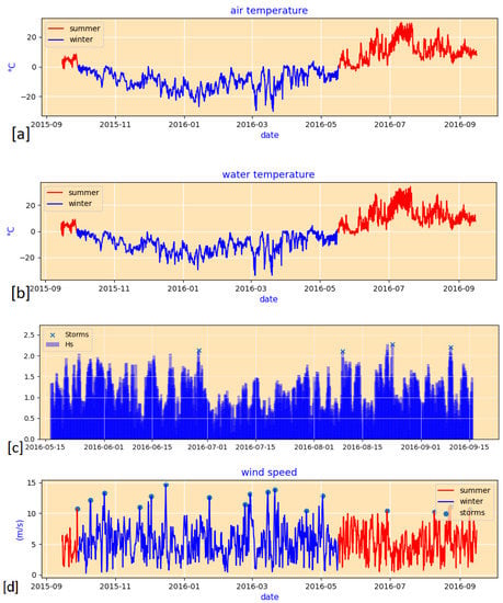
Figure 17.
The environmental forcing during the calibration cases is shown. [a] The air temperature of the study area is shown; summer with a red line and winter with a blue line. Winter started on 28 September and ended on 16 May the following year. During the summer of 2016, temperature reached 28 °C. The year 2016 was the hottest in recent decades. [b] Sea-surface temperature is shown, summertime with a red line and winter with a blue line. The phase lag between air and sea-surface temperature is minimal. [c] The wave conditions at the BC2 boundary during summer, the input for the XBeach, are shown. The storms are marked with ‘x’. [d] Wind speed and storms are shown. Wind speed is higher during the winter.
4.3.1. Upper and Lower Limit of the Mean Sea Level
The water level () at boundary BC2 (see Figure 1) is updated at every timestep. We estimate at the BC2 boundary by superimposing water level changes due to tide() and storm surge() on the mean sea level (). At the BC2 boundary, the water level () is treated as the boundary condition for the XBeach, expressed by the following equation:
where is the mean sea level, which is constant during the simulation (not a function of time), denotes tidal water-level changes at three-hour intervals (interpolated from the measurement), and is the storm surge level estimated at three-hour intervals by the storm surge submodule. For calibration, we employ the field measurements of sea level using the Russian State Geodetic Coordinate System (GSK-2011), which is also used as a datum for the numerical model. The values of and are not subject to calibration. The upper and lower limits of are the constraints imposed from field observations: (1) the water level does not touch the base of the bluffs during high tide on a calm day (upper limit of ), and (2) the length of the beach from the base of bluffs to the swash zone varies from 40 to 70 m (lower limit of ).
4.3.2. Upper and Lower Limit of the Convective Heat Transfer Coefficient
The convective heat transfer coefficient differs between the four sections (see Figure 4). In Section 4.2, we calibrated the for bluff surface. The remaining three other values are calibrated using trials and errors to match the total erosion volume. As a starting point for the value for water, we follow the model of Kobayashi et al. [36] as follows:
where a is the empirical parameter equal to 0.5, is the wave friction factor, is the volumetric heat capacity of seawater, is the fluid velocity and F is the parameter depending on the turbulence and Prandtl number. Kobayashi et al. [36] estimated the value of within the range of 500 to 800 W/mk.
For the of air of bluff slope and dry portion of the beach, the initial value of iteration is determined by using the equation for the forced convection of a turbulent flow over a flat plate:
where is the Nusselt number, is the thermal conductivity of the fluid, L is the characteristic length, is the Reynolds number, and is the Prandtl number. Using Pr = 0.71 for air, we estimate the initial value of to be approximately 25 W/mk.
4.3.3. Upper and Lower Limit of the Critical Slope ()
The slumping process inside the numerical model is controlled and triggered using one single parameter, the critical slope (), as mentioned in Equation (8). In this study, we calibrated the value of from the field observations. Alternatively, one can use numerical thermo-mechanical models, coupled with mechanical strength and thermal energy balance module ([50,51] or similar model) to perform slope stability of the bluffs and estimate the value of . The calibration is achieved by running the model with various values of within an acceptable range and then selecting the value that yields the closest estimate of total erosion volume and the profile shape. We estimated initial values for the trials from field measurements of the coastal profiles. The bluff height and bluff slope of 30 measurements are shown in Figure 18. The coastal profiles shown in the figure present observations that were free of snow at the time of measurement. These measurements were taken between 2012 and 2017 on several profiles of S#1 and S#2. The slope of the profiles varies from 0.1 to 1.1. A distinct difference is visible between the bluff slopes of zones S#1 and S#2. The coastal profiles are measured at the end of the summer when the thermodenudation is almost complete. We infer that the slopes of the bluff faces are near-stable slopes, and thus, the critical slope should be more than these measured slopes. We also note that the profiles at S#2 have a greater bluff height and steeper slope. We used a lower limit of Figure 18 for 0.2 and 0.4 for the S#1 and S#2, respectively. The upper limit was set at 0.45 and 0.8 for S#1 and S#2. The value of Figure 18 directly affects the value of erosion volume and shape of the bluff surface.
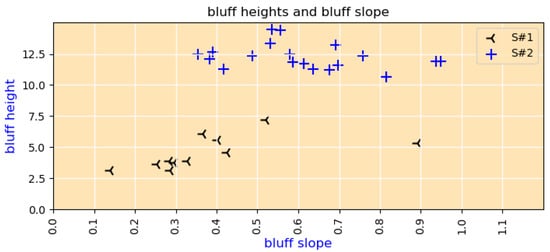
Figure 18.
Relation between the bluff height and bluff slope in the study area.
4.4. Calibration Result
Application of the environmental forcing iterations is performed with the calibrated parameters to match the simulation outcome to the three targets: net erosion volume, crest retreat and bluff slope as closely as possible. A summary of the calibrated values of the parameters is shown in Table 3. In the upcoming sections, we discuss the results of the calibration.
Table 3.
Summary of the calibrated parameters.
A summary of the calibration results with error measurements is shown in Table 4. The numerical model overestimates erosion volumes for both cases.
Table 4.
Summary of the calibration of case#1 and case#2. (td = thermodenudation and ta = thermoabrasion).
4.4.1. Prediction of Erosion
The simulated erosion volume for case#1 and case#2 differ from the measurements by 17.9% and 18.3%, respectively (Figure 19 and Figure 20). Thermoabrasion (ta) is the dominating mechanism, contributing 75.78% of cumulative erosion volume, whereas, for case#2, thermoabrasion (ta) is 59.18%. Four collapses are simulated for case#1, but for case#2, two collapses are triggered within the model. The values for the case#2 are also less frequent ( values over 20 cm are shown in the secondary axis). The sediment influx by thermodenudation is nearly three times greater for case#2 compared with case#1. Since the water level () is the same for both cases, we can deduce that the higher sediment influx by thermodenudation changes the nearshore morphology and influences the rate of thermoabrasion.
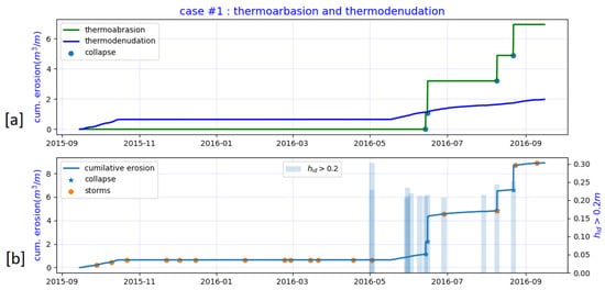
Figure 19.
Results of the calibration of Case#1. sub-figure [a]:Cumulative thermoabrasion and thermodenudation are shown separately. The sudden jumps in the erosion volumes indicate a bluff collapse by thermoabrasion. sub-figure [b]:The erosion volume from the measurement was 7.04 m/m−width, whereas the model simulated erosion of 8.3 m/m−width. Thermodenudation contributes 2.01 out of 8.3 m/m−width. Four collapses are simulated, and thermoabrasion contributes 75.7% of the erosion.
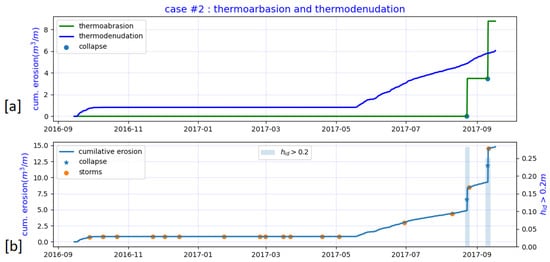
Figure 20.
Results of the calibration of Case#2. sub-figure [a]:Cumulative thermoabrasion and thermodenudation are shown separately. sub-figure [b]:The erosion volume from the measurement was 12.51 m/m−width, whereas the model simulated erosion volume was 14.8 m/m−width. Thermodenudation contributes 6.04 out of 14.8 m/m−width, about three-times greater than case#1. The bluff slope is steeper (0.9 vs. 0.4) and the bluff height is higher (13 m vs. 6 m). Two collapses are simulated and thermoabrasion contributes 59.18% of the erosion.
The two collapses in case#2 are in sync with storms. Case#1 has two additional collapses at the beginning of summer. The largest storm surge occurred during May, which did not result in any collapse. The thermal driving force of niche growth: the temperature of the water was not warm enough to rapidly grow the niche. We also notice the values are spiked and not continuous, which is in line with our assumption that only during storm surges can water reach the base of the bluffs.
4.4.2. Prediction of Crest Retreat
The secondary aim of the simulation is to predict the crest retreat of the bluffs. The crest retreat of the Arctic coast is retrogressive, i.e., always retreating as there is no restoration mechanism such as the dune systems of the sandy beaches in warmer climates. The crest of the bluff is always moving towards the land. The annual crest retreat rate is important for predicting vulnerability and associated risks. For case #1, the crest retreat rates were 4.1 m. The model predicts crest retreats of 3.9 m (Figure 21a). For case#2, the simulation predicted a crest retreat of 4 m (Figure 21b).
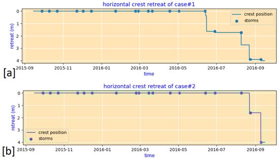
Figure 21.
The crest retreat as a time series is shown. sub-figure [a]: The crest retreats coincide with the bluff collapses. The sudden drops are due to thermoabrasion, which contributed the most to the retreat. sub-figure [b]: Similar pattern is visible for Case#2.
4.4.3. Prediction of the Shape of Coastal Profile
Secondary aim of the calibration is to forecast the shape of the profile at the bluff face and the elevation of the beach. The elevation of the beach is crucial since it affects the inundation depth (), which in turn controls the thermoabrasion. The performance of the model for case#1 is shown in Figure 22. Before estimating the RMSE value, we ‘normalise’ the profile around the middle of the bluff slope. Hence, the RMSE values are only related to the shape of the profile, and not associated with the position of the bluff.
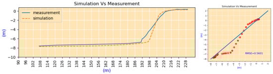
Figure 22.
Case#1: Prediction of the coastal profile shape after normalising the simulation around the middle of the bluff slope. The RMSE of the prediction is 0.56 m.
For case#1, we observe that the simulation predicted a slope slightly steeper than the measurement. The predicted elevation of the beach was close to the measurements, although it overestimated the erosion by sediment transportation. The deviation is highest near the base of the bluff; errors near the beach are negligible. The model overestimates the erosion at the base of the bluffs.
For case#2, shown in Figure 23, the model simulates the slope as much as the prediction. The simulated values deviated near the cliff points and the bluff base. The prediction at the beach was close. The RMSE values are higher for case#2.
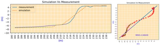
Figure 23.
Case#2: Prediction of the coastal profile shape after normalising the simulation around the middle of the bluff slope. The RMSE of the prediction is 0.88 m.
5. Validation
We apply the calibrated model to another three sets of measurements to validate the model. The new cases are summarised in Table 5. Case#3 and case#4 are from profiles#1 and #8 for 2016–2017. Case#5 is from the two measurements of 2012 and 2017 on profile#1. Case#5 is selected to examine the performance of the numerical model for simulating long-term erosion. The measured erosion volume and crest retreats of all the cases are shown in Appendix G.
Table 5.
A summary of the three cases for validation.
5.1. Methodology of the Validation
The calibrated parameters in Table 3 are used without any changes. The time series of the input parameters: air and water temperature, wind speed, and tides are updated. The initial thawing depths for case#3 and case#4 are used from the previous simulations (the thawing depth of the last timestep for case#1 and case#2). For case#5, the initial thawing depth was taken as zero because the case starts in June, not September. From the thawing-depth patterns of cases #1 and #2, we estimate that the thawing depth in June is zero.
5.2. Validation Results
A summary of the simulation results is shown in Table 6. The results show a good agreement with the measurements.
Table 6.
Summary of the validation cases.
5.2.1. Validation of Permafrost Thawing Module
The permafrost thawing module is calibrated by seeking minimum RMSE error from the measurements of summer 2017. The module is validated using the thawing depth measurements of summer 2014 from the same borehole. The thawing depth simulation mimics the field measurements (see Figure 24). The simulation could not properly capture the duration of thawing; however, the depth is captured quite accurately. The RMSE error is 0.07 m.
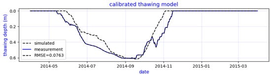
Figure 24.
Validation of the thawing module is completed using measurement of the summer of 2014.
5.2.2. Validation of Case#3
A summary of the validation results is shown in Figure 25. The cumulative erosion of the profile reaches 25.8 m/m−width, which is slightly underestimated by the simulation. The erosion is dominated by thermoabrasion, but the contribution from thermodenudation increased from the previous year, from 24.3% to 33.22% (case#1). The rate of thermodenudation was higher during the summer of 2017. However, the prediction of the beach elevation deviated from the measurements. The shape of the bluff face was irregular, which the model failed to capture. Similar to the other cases, the deviation is higher near the base.
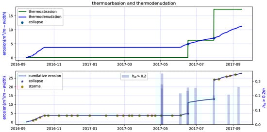
Figure 25.
Validation results for case#3. Thermoabrasion is 17.23 of 25.8 mm−width; 66.78% of the total erosion. The collapses are fewer in number.
5.2.3. Validation of Case#4
The cumulative erosion volume simulated by the model for case#4 is shown in Figure 26; the erosion is dominated by thermoabrasion (75.17%). The model estimated an erosion volume of 15.1 m/m−width, which is overestimated from the measurement of 11.81 m/m−width. Compared with case#2, case#4 demonstrated different behaviour. Thermoabrasion dominated the erosion mechanism with one initial big collapse.
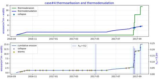
Figure 26.
Validation results for case#4.
5.2.4. Case#5: Simulation of Long-Term Erosion
The application of the model for the long-term erosion simulation is demonstrated by case#5. The simulation duration of the case is five years and four months. The simulation results are shown in Figure 27.
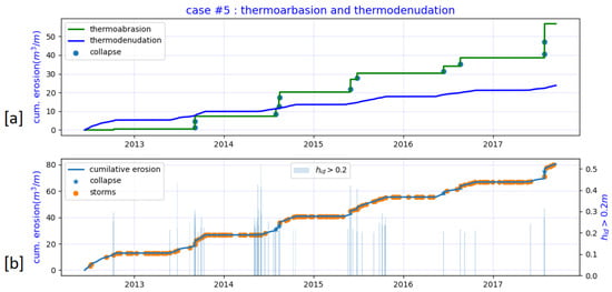
Figure 27.
Validation results for case#5.sub-figure [a]: The cumulative thermoabrasion and thermodenudation is shown separately. Thermoabrasion is the dominating mechanism; similar to earlier cases. sub-figure [b]: The combined erosion volume is 80.5 m/m−width which is over estimation of measurement.
The erosion pattern of case#5 is similar to the other cases. The erosion is dominated by thermoabrasion (70.68%). The thermodenudation rate differs each year. The values during the simulation are shown in the secondary y-axis of Figure 27b. We observe higher values for the earlier years; the highest is observed during the summer of 2014. The effect of the higher values of 2014 did not translate to many bluff collapses. The bluff collapse by niche growth requires a positive value, but the intensity of the erosion does not depend on the frequency and magnitude of the values.
Deviation of the profile shape is shown in Figure 28. The deviation is higher at cliff points and bluff bases. During the five-year simulation, the beach elevation was simulated to be lower than the measurements; the deviation was nearly 0.3 m, whereas the average deviation at the grid points was 0.86 m (RMSE).
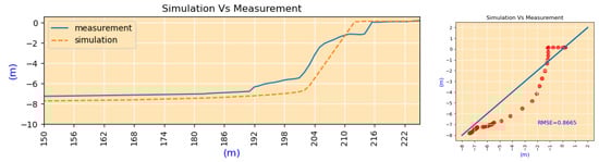
Figure 28.
Shape of the profile after normalising. The RMSE value was estimated to be 0.86.
5.2.5. The Effect of Environmental Forcing on Erosion
In Figure 29, the air temperature and simulated cumulative erosion are drawn. The upwards zero crossing of the air temperature and the inception of the erosion in the summer have a small phase lag. The erosion rate correlates with air temperature; higher air temperature leads to increased erosion. At the end of the summer, the erosion stops as soon as the air temperature exhibits downwards zero crossing.
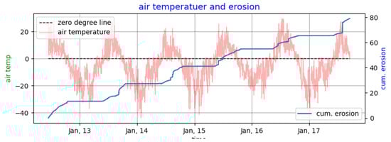
Figure 29.
Air temperature and cumulative erosion (simulation).
The thawing index of air is used in many empirical equations concerning the thawing of permafrost and erosion. Figure 30 draws the measured cumulative thawing index of case#5 juxtaposed with the simulated cumulative erosion. The correlation between the two parameters is very strong even though the thawing index is only one of the environmental forcing parameters of erosion. The cause of the erosion can be partly attributed to the thawing index. We cannot establish a direct causation-relation of the thawing index of air with thermoabrasion; warm air has almost no immediate effect on erosion by thermoabrasion. From the simulation result, we notice that even though erosion is dominated by thermoabrasion, a strong correlation exists between the cumulative thawing index and cumulative erosion.
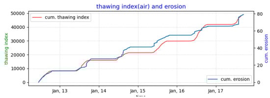
Figure 30.
Cumulative thawing index and erosion (simulation).
However, the wind speed and the simulated cumulative erosion of case#5 are not correlated (Figure 31). The wind speeds are higher during the winter when there is no erosion. The bluff collapses (creating a jump on the cumulative erosion) rarely coincide with the storms of the summer. We can infer that the bluff collapse by thermoabrasion is not dominated by storms in the summer; instead, a combination of various environmental forcing results in bluff failure, justifying the inclusion of hydrodynamic and morphological submodules into the numerical model of Arctic coastal erosion.
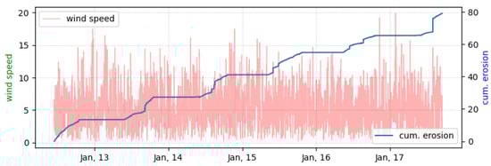
Figure 31.
Wind speed and cumulative erosion (simulation).
6. Sensitivity Analysis of the Model
We cannot validate all the modules individually since the measurements are only available once a year. Only the permafrost temperature inside the bluffs is measured continuously throughout the year. The temperature measurements yield a continuous year-round measurement of thawing depth, using which we can calibrate and validate the thawing module (Section 4.2). Thermoabrasion is episodic; pre and post-bluff-collapse measurements are essential to validate. Considering the scarcity of measurements to identify and discern the individual effect of the coastal processes, a sensitivity analysis is undertaken to demonstrate the behaviour of the numerical model and its potential applicability.
6.1. Base Case
Sensitivity analysis is performed on a base case, and some conclusions are inferred. Two approaches are adopted: (a) turning off a process and comparing it with the base case and (b) amplifying or damping one environmental forcing to observe the deviation from the base case. The base case is shown in Figure 32. The calibrated model is used to simulate the erosion of a hypothetical coastal profile over a period of 31.25 days, from 7 June 2016 to 8 July 2016. Environmental forcings are taken from NOAA reanalysis [40]. The profile has a bluff slope of 0.35, and a height of around 7 m. The base case is developed in such a way that one single mechanism does not dominate; thermoabrasion and thermodenudation are almost equal. The environmental forcing and erosion patterns are shown in Appendix H.
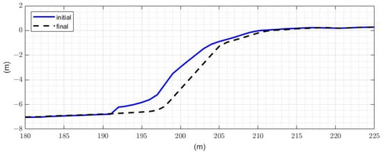
Figure 32.
Profile of the base case.
6.2. The Effect of Waves
The wave is the prominent mechanical driver of both erosion mechanisms. When we turn off the wave inside the XBeach, the values become very small to non-existent (Figure 33). No sediment transport along the cross-shore is simulated, eventually stopping thermodenudation by stabilizing the slope. The model detects almost no erosion as a result. We can infer the following:
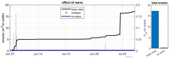
Figure 33.
The effect of waves on erosion.
- Thermoabrasion is controlled by both mechanical and thermal driving forces; the absence of one of the driving forces can withhold thermoabrasion.
- Mechanically driven forces do not control thermodenudation, i.e., they are not the limiting factor, but nearshore hydrodynamics can influence the rate of thermodenudation.
- Without the presence of waves, no bluff collapse occurs even when the model simulates positive values of ; indicating the importance of the combination of thermal and mechanical drivers.
Figure 34 shows the effect of the amplitude of the wave heights () at BC2 as an environmental forcing. A 20% increase in the significant wave height increases the cumulative erosion by more than 30% (qualitative assessment) as simulated by the model. The bluff collapses are more frequent and occur earlier in the summer when amplitudes are increased. Thermodenudation also increases as stronger waves enable a faster removal of the thawed materials from the bluff base.
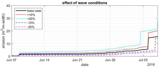
Figure 34.
The effect of wave inputs on erosion.
6.3. The Effect of Niche Growth
When we turn off the niche growth module, the model essentially converts to a thermodenudation model ignoring thermoabrasion even when the other modules of thermoabrasion are active. Figure 35 describes the result where erosion is only allowed by removing the sediments from the base via waves and currents, dominating by thermodenudation. We notice an initial high erosion. The frequent values indicate that the erosion is due to waves and currents removing the thawed material from the base of the bluffs and beaches.
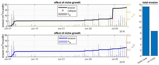
Figure 35.
Effect of the niche-growing process on erosion.
6.4. The Effect of Slumping Process
The results of turning off the slumping module are shown in Figure 36. The model allows the removal of sediments from the beach, but the influx from the slumping module is turned off. The result shows that the erosion initially has smaller values than the base case. However, the erosion volume increased significantly later in summer with frequent collapses. A comparison of the values reveals that higher and more frequent are observed for this case, indicating the importance of the influx of sediments from the thermodenudation as an erosion-resisting mechanism in the model. The sediment influx from the slumping elevates the base and reduces the probability of thermoabrasion. Thus, two erosion mechanisms are intertwined.
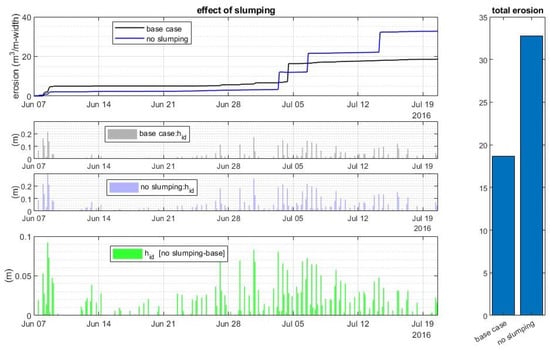
Figure 36.
Effect of the slumping process on erosion.
6.5. The Effect of Tide
Water level fluctuation due to tide () is simulated in XBeach as one of the input parameters. Figure 37 depicts the effect of excluding tide from the model. In our study, area, the tidal range is 70 centimetres, so the effect of the tidal fluctuation on the output of the numerical model appears small. The deviation from the base case is not very high. Both the thermodenudation and thermoabrasion are reduced, and the bluff collapses are delayed as values become smaller with lower frequency.
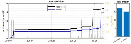
Figure 37.
The effect of tide on erosion.
6.6. The Effect of Water Level
The model is highly sensitive to water level (, defined using Equation (10)). The incremental water level changes (10 cm) are shown in Figure 38. The frequency of the bluff collapse is related to the . The erosion volume shows a linear relation with the input parameter . The erosion volume increases about three times causing a 30 cm elevation in water levels.
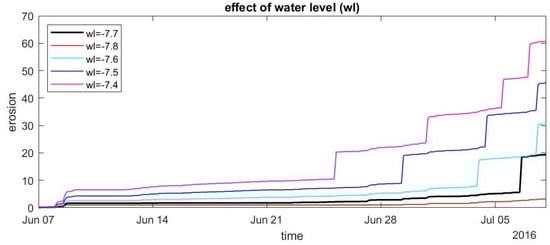
Figure 38.
The effect of water level inputs on erosion.
The effects of water and air temperature are shown in Appendix I. The results show that the air and water temperatures are not the limiting factor for both erosion mechanisms. The air and water temperatures act as an on/off switch inside the model since niche growth and permafrost thawing are impossible without a positive temperature.
7. Conclusions
This paper describes a comprehensive process-based model that simulates Arctic coastal erosion, including hydrodynamic forcing from the sea. The model is constructed by coupling XBeach with in-house thermal modules. The model includes the physical processes as submodules under the two major erosion mechanisms: thermodenudation and thermoabrasion. A feedback mechanism is established between the submodules so that the model can simulate thermodenudation and thermoabrasion simultaneously.
The numerical implementation of the model is described briefly, and the workflow is explained. We calibrate the model using field measurements from Baydaratskya Bay in the Kara Sea, Russia. The simulation by the calibrated model agrees reasonably with the field measurements. The analysis of the erosion patterns reveals the erosion mechanism is dependent on the nearshore hydrodynamics and morphological changes. Hence, including a proper hydrodynamic and sediment transport model to simulate Arctic coastal erosion significantly improves the fidelity.
The following conclusions can be made from the calibration process of the numerical model:
- 1.
- Erosion during the winter is negligible or absent. Barnhart et al. [30] concluded in their model that low erosion occurs at the end of summer and beginning of fall for the coast of Alaskan Beaufort Sea whereas our numerical model for Baydaratskya Bay in Kara sea simulates higher erosion at the middle and end of summer.
- 2.
- There is a slight phase lag between the commencement of summer (measured by air temperature) and the beginning of slumping. The air temperature had an upwards zero crossing at the end of May, but thawing began after June in both cases #1 and #2.
- 3.
- Smaller sudden spikes in air and water temperature at the beginning of summer do not contribute to thermodenudation. The model also does not show any immediate response to the spikes of temperature anomalies. This behaviour indicates that the limiting factor for thermal energy transfer and thawing of permafrost is the energy requirement for the latent heat of the transformation from ice to water.
- 4.
- Thermodenudation is continuous and of lower intensity, whereas thermoabrasion causes spikes in erosion volume. The limiting factors for thermodenudation and thermoabrasion are, respectively, the latent heat requirement and water depth at the base of the bluffs ().
The model is validated by another three sets of observations, two short-term (one year) and one long-term (five years). We demonstrate that the model can simulate long-term erosion with the same level of fidelity. We infer the following concluding remarks from the results of the simulations:
- 1.
- The results of the numerical model suggest that thermoabrasion is a complex process and does not demonstrate a linear relation with the intensity of storms. In other words, the strongest storm does not necessarily lead to a collapse. A bluff collapse by a wave-cut niche results from a combination of the nearshore beach profile, storm surge duration, water temperature, and bluff geometry. A similar observation was made by Barnhart et al. [30] for the thermoabrasion numerical model of the Alaskan Beaufort coast.
- 2.
- The two consecutive bluff collapses routinely have an interval between them, and the time lapse between the two collapses is four to six weeks. The sediments released from the collapsed bluff alter the elevation near the swash zones, reducing the probability of inundating the beach with warm water and resulting in slow niche growth. The model by Ravens et al. [29] considered a numerical elevation of the beach by about 0.28 m to calibrate the model and achieve optimised calculation. In contrast, the model proposed herein assumes the sediment from the bluffs increases the elevation of the beach and the elevation is controlled by the morphodynamic module (XBeach).
- 3.
- The parameter inundation depth, , acts as an on–off switch for thermoabrasion; however, the numerical model does not show a clear relationship between the magnitude of and erosion. Our model agrees with the previous observation of Ravens et al. [29] that overall crest retreat is controlled by the niche erosion process.
- 4.
- The erosion rate of thermodenudation was found to be approximately 0.4 m/month for low bluff-height profiles in zone S#1. The erosion rate by thermodenudation for the zones with high bluff was estimated to be close to 1 m/month. The erosion rate of thermodenudation does not show a strong relationship with the thawing depth ().
We conclude the following from the sensitivity analysis using a base case:
- 1.
- The hydrodynamic forcing, especially wave condition, plays a vital role in the erosion mechanism; hence the inclusion of the nearshore hydrodynamics and morphological changes is important.
- 2.
- The limiting factor for the rate of thermodenudation is found to be the critical slope (). In the case of thermoabrasion, the limiting factor was .
- 3.
- Thermodenudation and thermoabrasion are intertwined; one mechanism can affect the other. For beaches where the two mechanisms are active, this feedback should be taken into consideration.
We demonstrate that coupling the physical processes as submodules to simulate Arctic coastal erosion model erosion can produce realistic coastline erosion rates. It is possible to couple the model with globally available climate reanalysis data. The simulation results are within the same order of magnitude as the field measurements. The model can be further improved by considering the following:
Future Development
- 1.
- The accumulation and melting of snow and related water flow are not exclusively modelled. Since there is no open water during the winter and coastal erosion is negligible, we did not model the effect of snow. A snow module will improve the accuracy of the model.
- 2.
- The presence of sea ice was considered in a binary mode, where we ignored sea ice when the ice concentration was less than 20%, and it was assumed to not affect the waves. The damping effect of the floating ice on the waves may also improve the model’s fidelity.
- 3.
- The critical slope () is taken as depth-averaged for the profiles. One depth-averaged value is estimated for each zone in the study area. A matrix of values at different depths and geometries will increase the model’s accuracy.
- 4.
- The collapse of the bluff is predetermined. A finite element model at the bluff face may better predict the irregular bluff slope.
- 5.
- The model is applicable to the unlithified Arctic coasts since gravel is not included in the XBeach explicitly.
Supplementary Materials
The following supporting information can be downloaded at: https://www.mdpi.com/article/10.3390/jmse10111602/s1, File: A stand-alone module of slumping; written in Matlab.
Author Contributions
Conceptualization, M.A.I. and R.L.; methodology, M.A.I. and R.L.; software, M.A.I. and R.L.; validation, M.A.I. and R.L.; formal analysis, M.A.I.; investigation, M.A.I. and R.L.; resources, R.L.; data curation, M.A.I.; writing—original draft preparation, M.A.I. and R.L.; writing—review and editing, R.L.; visualization, M.A.I.; supervision, R.L; project administration, R.L.; funding acquisition, R.L. All authors have read and agreed to the published version of the manuscript.
Funding
This report was written as part of the EU H2020-funded Nunataryuk project (Grant: 773421), where it is filed as part of deliverable 6.4.
Institutional Review Board Statement
Not applicable.
Informed Consent Statement
Not applicable.
Data Availability Statement
Not applicable.
Acknowledgments
The toolbox developed by the OpenEarth community (https://openearth.community/about-oec, accessed on: 8 October 2021) allowed better control over XBeach. The team led by Vladislav Isaev from the Department of Geocryology, Lomonosov Moscow State University (MSU), Russia obtained the field observations with support from the project Sustainable Arctic Marine and Coastal Technology (SAMCoT), Norway and Norwegian University of Science and Technology (NTNU).
Conflicts of Interest
The authors declare no conflict of interest.
Appendix A. Definitions
Below are some geometric parameters defined to explain the Arctic coasts:
- 1.
- profile line: the surface line of the beach profile not including the snow or ice sheets. During the summer, the profile line is exposed to environmental parameters.
- 2.
- permafrost table: the thawing face of the permafrost. During the winter, the line is assumed to collide with the profile line. The difference between the beach line and the permafrost table is the thawing depth.
- 3.
- base point: the point at the end of the beach where a sudden change in the slope occurs. Typically, it stands above the tidal range and in calm conditions, water level can not reach the base point.
- 4.
- cliff point: the end of the bluff-face and beginning of the bluff-surface; a sudden change in the slope.
- 5.
- ice-wedge top point: the point at the surface where the ice-wedge polygon is visible on the surface.
- 6.
- ice-wedge bottom point: not necessarily the bottom point of the ice-wedge. It is the point from which we can assume the continuity of the bluff is broken by the ice wedge.
- 7.
- swash point/line: Where the average water depth for a timestep is less than 5cm. The point(1D) or line(2D) is assumed to be constant for one timestep.
- 8.
- thawing depth: The difference between the permafrost line and profile line, calculated for the grid points on the profile line and normal to the tangent on the point at the profile line.
Appendix B. Four Zones of the Coastal Profile
The four zones of the Arctic coast in terms of erosion, thermal energy transfers and involvement of various physical processes are described in Figure 2. The four zones are defined as follows:
- 1.
- bluff surface: it is the surface behind the cliff point . The slope in the zone is zero or close to zero. The surface is covered with vegetation during the summer. Subsidence due to the thawing of the permafrost is the major change in the profile. Thawing depth is dependent on the convection of air and solar radiation. We assume the erosion due to surface run-off is negligible (based on field observation). The bluffs are usually filled with ice-wedge polygons. The organic-active layer at the top of the surface has negligible shear strength but can contribute to the lower erodibility to surface run-offs.
- 2.
- bluff face: It is the steepest slope of the profile, in between the base point and cliff point and the most active part of the profile. The thawing process contributes directly to the mass loss by slumping and cliff retreat.
- 3.
- beach: The narrow beach in front of the bluff from the base point to the swash point . The thawed sediments accumulate on the beach. The collapsed bluffs fall on the beach. The beach is subject to inundation during the summer storms. The return currents created during the storms sort out the accumulated sediments and transport them offshore.
- 4.
- seabed: It is defined from the swash point to the offshore. The general direction of the sediment transport is offshore since there exist no restoration mechanisms at the Arctic beaches. The wave-induced particle movement is enough to transfer heat (convective heat transfer). The thawing depth is not the limiting factor, i.e., the permafrost lies quite deep. However, due to sea ice, sediment transport during the winter is negligible.
Appendix C. Numerical Schematisation of the Submodules
Appendix C.1. Modelling Storm Surge
Storm surge is modelled by discretising Equation (A1). The setup/surge level is assumed to be zero at the offshore boundary, where is the water level setup from the mean sea level. The surge level, is determined at a 3-h interval. The 3-h time-averaged wind speed is used as an input parameter. When the ice concentration near the sea, is above 20%, the surge is set to zero, assuming damping from the ice. The following equation determines the storm surge at each grid point.
The storm surge submodule is the steady-state solution of the following Equation [38]:
where g is the gravitational acceleration, is the mean water depth (time-averaged), is the Coriolis frequency of Earth, is the latitude of the study area (in radians), is the seawater density, V = depth-averaged alongshore water velocity, is the stress from the wind on the surface of the water, is the drag coefficient (), and is the wind speed at 10 m and is the pressure drop.
Equation (A1) is discretised using the forward Euler numerical scheme as follows:
The details of the numerical model of the steady state storm surge are provided by Barnhart et al. [30] in Supplementary text S1 available at: https://agupubs.onlinelibrary.wiley.com/action/downloadSupplement?doi=10.1002%2F2013JF002845&file=2013JF002845text01_March2014.pdf, accessed on 2 September 2022.
Appendix C.2. Modelling Slumping
The numerical schematisation of slumping is shown in Figure A1. The line ABCD was the original profile before slumping. Point A has a slope less than the critical slope (). The next grid point B has a slope greater than . Slumping occurred at point B, which resulted in the new line AB′C′D. The permafrost line WXYZ remained unchanged; however, the thawed layer thickness at grid points B and C changed due to slumping. The criterion to initiate slumping as described earlier:
where is the slope of the grid point j and is the critical slope of the grid point j.

Figure A1.
Numerical schematisation of slumping based on critical slope and fall by gravity only. The line ABCD is the profile line which had WXYZ permafrost line at various thawing depths of each grid point. The slope at point B is greater than which triggers the slumping and the new position for the point B at the same grid line is B′.

Let us assume, at the n-th timestep, the numerical submodule is checking whether slumping is triggered at each grid point. Using the critical slope criteria, the model finds point A, the i th grid point does not satisfy the criteria , then it checks the i + 1 th grid, the point B.
The slumping module is based on the following assumptions:
The slumping process is initiated by gravitational force only. We ignore the movement of thawed material by the water flow created as a result of permafrost thawing.
The constraints of the initiation of the slumping at the i + 1 th grid point (point B in the figure) are as follows:
- C1. No slumping occurs at the permafrost table, the line WXYZ, irrespective of the slope. The failure within permafrost is considered in the bluff stability submodule. This submodule only simulates until thawing depth.
- C2. The slope at the grid point before the i th cell (point A) has a lower slope than critical .
- C3. The n-th timestep has j number of iterations where j is any number iteration until Equation (A3) is no more satisfied.
- C4. For slumping at i-th grid point at j th iteration, the mass transfer is limited to two adjacent grid cells; points B and C are moved to B′ and C′.
- C5. As a result of slumping, the grid point in consideration, point B, will be subsided to B′, increasing the elevation of point C to C′.
- C6. The subsidence of point B is such that the area under the curve ABCD will be equal to the area AB′C′D so that the conservation of mass is maintained.
- C7. Rule C6 is overridden when the subsidence of point B′ is limited by the permafrost line. Point B is not allowed to be lowered than point X. If C6 is overridden, then point C will move and still maintain mass balance. In this case, the movement of the mass will be lower.
- C8. The slumping process is always triggered in the downward direction. If for n th timestep, if two grid points have a slope more than the critical value , slumping will be initiated at the grid point in the higher vertical position.
There is no limit to the iterations for each time step, i.e., the module will run until all the grid points in the profile satisfy the governing equation.
If the slumping occurs, it overrides the thawing depth, estimated by the thawing depth modules.
The workflow of the numerical model is shown in Figure A2. Each grid point is checked for the triggering condition, and then the profile is continuously updated until the last grid point. When all the grid points are examined, the numerical model allows for the next coupled module or next time step.

Figure A2.
Workflow of the slumping module.
Figure A2.
Workflow of the slumping module.

To demonstrate the governing rules mentioned earlier, the module is applied to a hypothetical case. The coastal profile has a 6m bluff height with a bluff slope of 0.5 (26.5°). The thawing depth is 1m at the bluff surface and beach, and 0.71 at the bluff surface.
- Figure A3a demonstrates the case when the is equal to the initial slope, i.e., no slumping can occur establishing the value acts as a triggering condition in the numerical model.
- Figure A3b demonstrate a case when we consider the = 0.4. The slumping occurred and part of the bluff surface was exposed (no thawing depth on the upper portion of the bluff surface).
- The effect of on the final profile is shown in Figure A3c. When we reduce the value to 0.3 from 0.4, keeping everything else the same, the exposed portion of the bluff surface got decreased. The slumped materials now moved further back on the beach.
- If we further decrease the value, the sediments are now distributed on almost 35 m along the beach (Figure A3d) and a large portion of the bluff surface is exposed.
- Figure A3e demonstrates a reduction in thawing depth on slumping. If the thawing depth is reduced to 0.5 m with a low value most of the bluff surface is exposed as a result.
- Figure A3f demonstrates the effect of very high thawing depth, the model behaviour is similar to active layer detachment, and a large portion of the thawed layer is moved.

Figure A3.
Application of the thawing module in some cases. (a) = 0.5, initial slope = 0.5, thawing depth = 1 m; (b) = 0.4, initial slope = 0.5, thawing depth = 1 m; (c) = 0.3, initial slope = 0.5, thawing depth = 1 m; (d) = 0.1, initial slope = 0.5, thawing depth = 1 m; (e) = 0.2, initial slope = 0.5, thawing depth = 0.5 m; (f) = 0.2, initial slope = 0.5, thawing depth = 2 m.

Appendix C.3. Modelling Bluff Stability
Four modes of failure cases are considered at each timestep. Three of them are the shear failure (mode#1 to#3) and the rest moment failure, the governing equations are described earlier. The failure modes are as follows (see Figure A4):
- 1.
- Mode#1: The failure line is CE (from the cliff point to the base point E). The bluff face got steeper as a result.
- 2.
- Mode#2: The failure line is GE. Point G is determined using the same slope of the bluff.
- 3.
- Mode#3: The failure line is FE. F is the lowest point of the ice-wedge polygon. The shear failure line is the FE.
- 4.
- Mode#4: The failure line is PE and PF. This is the moment failure mode.

Figure A4.
Stability of the overhanging bluffs.
Figure A4.
Stability of the overhanging bluffs.

Appendix D. Physical Properties of Permafrost
Table A1.
Particle size distribution in the study area.
Table A1.
Particle size distribution in the study area.
| Particle Size (%-mm) | 1.0–0.5 | 0.5–0.25 | 0.25–0.1 | 0.1–0.05 | 0.05–0.01 | 0.01–0.005 | <0.005 | <0.002 | <0.001 | Moisture (%) | Density (gm/cm) |
|---|---|---|---|---|---|---|---|---|---|---|---|
| Sample 1 | 0.2 | 1.0 | 59.5 | 24.1 | 7.4 | 0.5 | 0.5 | 1.5 | 5.2 | 29 | 2.63 |
| Sample 2 | 0.1 | 0.9 | 58.4 | 26.6 | 5.2 | 1.6 | 0.5 | 1.0 | 5.7 | 29 | 2.64 |
| Sample 3 | 0.1 | 0.1 | 64.9 | 23.6 | 3.2 | 0.3 | 0.5 | 1.2 | 6.1 | 29 | 2.64 |
| Sample 4 | 0.1 | 0.8 | 62.1 | 24.6 | 3.8 | 0.8 | 0.5 | 1.2 | 6.0 | 29 | 2.63 |
For the detailed field report, we refer to [49], accessible at https://www.researchgate.net/publication/322103499_Field_investigation_and_laboratory_analyses_Baydaratskaya_bay_2017, accessed on 14 September 2021.
Appendix E. Measurements of Thawing Depth

Figure A5.
Position of the borehole#4 on profile#3. Image source: SAMCoT report 2015.
Figure A5.
Position of the borehole#4 on profile#3. Image source: SAMCoT report 2015.

Nodes are positioned at 0, 5, 10, 16, 27, 35, 44, 55, 86, 100, 115, 130, 145, 164, 180, 204, 220 and 243 cm from the surface.
Trumpet curves for each month of 2014 are shown in Figure A6.

Figure A6.
Trumpet curves of the temperature within bluffs for each month.
Figure A6.
Trumpet curves of the temperature within bluffs for each month.

Appendix F. The Parameters of XBeach
The simulation time for every timestep is 10,900 s which is 3 h and 100 s. An additional 100 s is added to make sure the waves reach the shoreline. The simulation of morphological changes starts after 100 s. Using the ‘tstart’ parameters, it is controlled within XBeach.
Flow boundary condition parameters
front = abs_1d
back = abs_1d
wavemodel = stationary
tstop = 10,900
CFL = 0.900000
morfac = 1
morstart = 100
wetslp = 0.300000
dryslp = 0.700000
struct = 1
ne_layer = nebed.dep
bcfile = filelist.txt
outputformat = netcdf
tintp = 60
tintg = 60
tstart = 100

Figure A7.
The variable grid spacing along x-axis.
Figure A7.
The variable grid spacing along x-axis.

Appendix G. Coastal Profiles for Validation Cases
Even though cases#1, #3 and #5 are on the same profile#1, the erosion pattern is different for each case. In two consecutive years, the erosion pattern drastically changed between cases #1 and #3 (Figure A8a). The bluff slope of case#3 morphed into an uneven bluff slope. The bluff slope became steeper at the lower part near the bluff base, indicating that during the summer of 2017, the hydrodynamic forcing removed a large volume of sediments from the bluff base. Case#4 on profile#8 is relatively stable, but we note the lowering of the elevation of the beach (Figure A8b). Lowering beach elevation indicates that the beach was inundated frequently during the summer of 2017, a similar conclusion we made for case#3. Case#5 is a representation of long-term erosion (Figure A8c). The erosion of the beach was significant in this case; the profile is lowered by approximately 1.5 m around the 180-m mark. However, the base of the bluffs remains almost at the same level. No positive accretion value was recorded for any of the three cases, which suggests that the accumulated sediments must have been washed away by hydrodynamic forcing.

Figure A8.
Coastal profiles of cases#3, #4 and #5 are shown. (a) Case#3: Measurements are of profile P#1, from 2016 to 2017. (b) Case#4: Measurement of profile P#8, from 2016 to 2017. (c) Case#5: Measurement of profile P#1, from 2012 to 2017.
Figure A8.
Coastal profiles of cases#3, #4 and #5 are shown. (a) Case#3: Measurements are of profile P#1, from 2016 to 2017. (b) Case#4: Measurement of profile P#8, from 2016 to 2017. (c) Case#5: Measurement of profile P#1, from 2012 to 2017.

Appendix H. Base Case: Environmental Forcing

Figure A9.
Environmental forcing of the base case.
Figure A9.
Environmental forcing of the base case.


Figure A10.
Erosion of the base case.
Figure A10.
Erosion of the base case.

Appendix I. Effect of the Environmental Forcing
Appendix I.1. Effect of Seawater Temperature
The base case is modified to demonstrate the effect of water temperature. Instead of applying the environmental forcing as shown in Figure A9, a mean water temperature is used so that the deviation of the erosion volume over time can be identified. The mean seawater temperature of the base case was 6.65 C. We now apply 2 to 10 C with 2 C increment (Figure A11). The erosion with mean 6 C is considered the base case. For the base case, no bluff collapse is recorded. Bluff collapse is triggered for 8 C and 10 C, collapse for 10 C occurred just 12 h earlier (three timesteps). We can infer that unless the mean seawater temperature for this 32.5 days is over 6 C, it is unlikely any bluff collapse will occur. We also notice, for the first three cases, the erosion volume is almost the same, indicating the sea-water temperature is not an important factor for the thermodenudation of the bluff surface.

Figure A11.
The effect of water temperature inputs on erosion.
Figure A11.
The effect of water temperature inputs on erosion.

Appendix I.2. The Effect of Air Temperature
Similar to the sensitivity analysis of water temperature, the base case is modified to demonstrate the effect of air temperature on erosion volume. The mean air temperature of the earlier base case is 11.45 C. The air temperature for the modified base case is chosen as 10 C. The new base case is chosen in such a way that thermodenudation is the dominant erosion mechanism. Keeping all other environmental forcings unchanged, only air temperature is increased and decreased. The result is shown in Figure A12. The cases indicate in our model that air temperature at the beginning of summer may be the controlling parameter for erosion, but eventually, the difference due to air temperature is not significant. However, we can not reach a conclusion from this analysis since only the thermodenudation mechanism is considered in this analysis. Thermodenudation in the study area contributes nearly 20 to 30% of the erosion volume.

Figure A12.
The effect of air temperature inputs on erosion.
Figure A12.
The effect of air temperature inputs on erosion.

References
- Lantuit, H.; Overduin, P.P.; Couture, N.; Wetterich, S.; Aré, F.; Atkinson, D.; Brown, J.; Cherkashov, G.; Drozdov, D.; Forbes, D.L.; et al. The Arctic coastal dynamics database: A new classification scheme and statistics on Arctic permafrost coastlines. Estuaries Coasts 2012, 35, 383–400. [Google Scholar] [CrossRef]
- Gibbs, A.E.; Richmond, B.M. National Assessment of Shoreline Change: Historical Shoreline Change along the North Coast of Alaska, US-Canadian Border to Icy Cape; US Department of the Interior, US Geological Survey: Washington, DC, USA, 2015.
- Isaev, V.; Koshurnikov, A.; Pogorelov, A.; Amangurov, R.; Podchasov, O.; Sergeev, D.; Buldovich, S.; Aleksyutina, D.; Grishakina, E.; Kioka, A. Cliff retreat of permafrost coast in south-west Baydaratskaya Bay, Kara Sea, during 2005–2016. Permafr. Periglac. Process. 2019, 30, 35–47. [Google Scholar] [CrossRef]
- Gibbs, A.; Richmond, B.; Erikson, L.; Jones, B. Long-term retreat of coastal permafrost bluffs, Barter Island, Alaska. In Proceedings of the 5th European Conference on permafrost, EUCOP5, Chamonix, France, 23 June–1 July 2018; Volume 1, pp. 1–2. [Google Scholar]
- Jones, B.M.; Arp, C.D.; Jorgenson, M.T.; Hinkel, K.M.; Schmutz, J.A.; Flint, P.L. Increase in the rate and uniformity of coastline erosion in Arctic Alaska. Geophys. Res. Lett. 2009, 36. [Google Scholar] [CrossRef]
- Jones, B.; Bull, D.; Farquharson, L.; Buzard, R.; Arp, C.; Grosse, G.; Romanovsky, V. A decade of annual permafrost coastal observations indicate changes in the Arctic System. Environ. Res. Lett. 2018, 13, 1–13. [Google Scholar]
- Ogorodov, S.; Aleksyutina, D.; Baranskaya, A.; Shabanova, N.; Shilova, O. Coastal erosion of the Russian Arctic: An overview. J. Coast. Res. 2020, 95, 599–604. [Google Scholar] [CrossRef]
- Barnhart, K.; Overeem, I.; Anderson, R.S. The effect of changing sea ice on the physical vulnerability of Arctic coasts. Cryosphere 2014, 8, 1777–1799. [Google Scholar] [CrossRef]
- Stroeve, J.; Notz, D. Changing state of Arctic sea ice across all seasons. Environ. Res. Lett. 2018, 13, 103001. [Google Scholar] [CrossRef]
- Serreze, M.; Barrett, A.; Stroeve, J.; Kindig, D.; Holland, M. The emergence of surface-based Arctic amplification. Cryosphere Discuss. 2008, 2, 601–622. [Google Scholar] [CrossRef]
- Cohen, J.; Screen, J.A.; Furtado, J.C.; Barlow, M.; Whittleston, D.; Coumou, D.; Francis, J.; Dethloff, K.; Entekhabi, D.; Overland, J.; et al. Recent Arctic amplification and extreme mid-latitude weather. Nat. Geosci. 2014, 7, 627–637. [Google Scholar] [CrossRef]
- Nielsen, D.; Pieper, P.; Barkhordarian, A.; Overduin, P.; Ilyina, T.; Brovkin, V.; Baehr, J.; Dobrynin, M. Increase in Arctic coastal erosion and its sensitivity to warming in the twenty-first century. Nat. Clim. Chang. 2022, 12, 263–270. [Google Scholar] [CrossRef]
- Rowland, J.; Jones, C.; Altmann, G.; Bryan, R.; Crosby, B.; Hinzman, L.; Kane, D.; Lawrence, D.; Mancino, A.; Marsh, P.; et al. Arctic landscapes in transition: Responses to thawing permafrost. Eos Trans. Am. Geophys. Union 2010, 91, 229–230. [Google Scholar] [CrossRef]
- Overeem, I.; Anderson, R.S.; Wobus, C.W.; Clow, G.D.; Urban, F.E.; Matell, N. Sea ice loss enhances wave action at the Arctic coast. Geophys. Res. Lett. 2011, 38. [Google Scholar] [CrossRef]
- Steele, M.; Ermold, W.; Zhang, J. Arctic Ocean surface warming trends over the past 100 years. Geophys. Res. Lett. 2008, 35. [Google Scholar] [CrossRef]
- Holland-Bartels, L.; Pierce, B. An Evaluation of the Science Needs to Inform Decisions on Outer Continental Shelf Energy Development in the Chukchi and Beaufort Seas, Alaska; Technical Report; US Geological Survey: Reston, VI, USA, 2011.
- Günther, F.; Overduin, P.P.; Yakshina, I.A.; Opel, T.; Baranskaya, A.V.; Grigoriev, M.N. Observing Muostakh disappear: Permafrost thaw subsidence and erosion of a ground-ice-rich island in response to arctic summer warming and sea ice reduction. Cryosphere 2015, 9, 151–178. [Google Scholar] [CrossRef]
- Irrgang, A.M.; Lantuit, H.; Manson, G.K.; Günther, F.; Grosse, G.; Overduin, P.P. Variability in rates of coastal change along the Yukon coast, 1951 to 2015. J. Geophys. Res. Earth Surf. 2018, 123, 779–800. [Google Scholar] [CrossRef]
- Jones, B.M.; Irrgang, A.M.; Farquharson, L.M.; Lantuit, H.; Whalen, D.; Ogorodov, S.; Grigoriev, M.; Tweedie, C.; Gibbs, A.E.; Strzelecki, M.C.; et al. Coastal Permafrost Erosion. Arct. Rep. Card 2020, 15. [Google Scholar]
- Jones, B.M.; Hinkel, K.M.; Arp, C.D.; Eisner, W.R. Modern erosion rates and loss of coastal features and sites, Beaufort Sea coastline, Alaska. Arctic 2008, 61, 361–372. [Google Scholar] [CrossRef][Green Version]
- Landrum, L.; Holland, M.M. Extremes become routine in an emerging new Arctic. Nat. Clim. Chang. 2020, 10, 1108–1115. [Google Scholar] [CrossRef]
- Are F, E. Thermal abrasion of sea coast. Polar Geogr. Geol. 1988, 12, 1–157. [Google Scholar] [CrossRef]
- Squire, V.A.; Vaughan, G.L.; Bennetts, L.G. Ocean surface wave evolvement in the Arctic Basin. Geophys. Res. Lett. 2009, 36. [Google Scholar] [CrossRef]
- Kobayashi, N. Formation of thermoerosional niches into frozen bluffs due to storm surges on the Beaufort Sea coast. J. Geophys. Res. Ocean. 1985, 90, 11983–11988. [Google Scholar] [CrossRef]
- Russell-Head, D. The melting of free-drifting icebergs. Ann. Glaciol. 1980, 1, 119–122. [Google Scholar] [CrossRef]
- White, F.M.; Spaulding, M.L.; Gominho, L. Theoretical Estimates of the Various Mechanisms Involved in Iceberg Deterioration in the Open Ocean Environment; Technical Report; Rhode Island Univ. Kingston: Kingston, RI, USA, 1980. [Google Scholar]
- Bull, D.L.; Bristol, E.M.; Brown, E.; Choens, R.C.; Connolly, C.T.; Flanary, C.; Frederick, J.M.; Jones, B.M.; Jones, C.A.; Ward Jones, M.; et al. Arctic Coastal Erosion: Modeling and Experimentation; Technical Report; Sandia National Lab. (SNL-NM): Albuquerque, NM, USA, 2020. [Google Scholar]
- Hoque, M.A.; Pollard, W.H. Arctic coastal retreat through block failure. Can. Geotech. J. 2009, 46, 1103–1115. [Google Scholar] [CrossRef]
- Ravens, T.; Jones, B.; Zhang, J.; Arp, C.D.; Schmutz, J.A. Process-based coastal erosion modeling for drew point, North Slope, Alaska. J. Water. Port Coastal Ocean. Eng. 2012, 138, 122–130. [Google Scholar] [CrossRef]
- Barnhart, K.R.; Anderson, R.S.; Overeem, I.; Wobus, C.; Clow, G.D.; Urban, F.E. Modeling erosion of ice-rich permafrost bluffs along the Alaskan Beaufort Sea coast. J. Geophys. Res. Earth Surf. 2014, 119, 1155–1179. [Google Scholar] [CrossRef]
- Hoque, M.A.; Pollard, W. Thermal and mechanical erosion along ice-rich Arctic coasts. In Proceedings of the 9th Intl. Conf. on Permafrost, Fairbanks, Alaska, 29 June–3 July 2008; pp. 741–746. [Google Scholar]
- Ravens, T.; Ulmgren, M.; Wilber, M.; Hailu, G.; Peng, J. Arctic-capable coastal geomorphic change modeling with application to Barter Island, Alaska. In Proceedings of the OCEANS 2017-Anchorage, Anchorage, AK, USA, 18–21 September 2017; pp. 1–4. [Google Scholar]
- Deltares. XBeach. 2022. Available online: https://oss.deltares.nl/web/xbeach/release-and-source (accessed on 10 October 2020).
- Frederick, J.; Mota, A.; Tezaur, I.; Bull, D. A thermo-mechanical terrestrial model of Arctic coastal erosion. J. Comput. Appl. Math. 2021, 397, 113533. [Google Scholar] [CrossRef]
- Rolph, R.; Overduin, P.P.; Ravens, T.; Lantuit, H.; Langer, M. ArcticBeach v1. 0: A physics-based parameterization of pan-Arctic coastline erosion. Geosci. Model Dev. Discuss. 2021, 1–26. [Google Scholar]
- Kobayashi, N.; Vidrine, J.; Nairn, R.; Soloman, S. Erosion of frozen cliffs due to storm surge on Beaufort Sea Coast. J. Coast. Res. 1999, 15, 332–344. [Google Scholar]
- Irrgang, A.M.; Bendixen, M.; Farquharson, L.M.; Baranskaya, A.V.; Erikson, L.H.; Gibbs, A.E.; Ogorodov, S.A.; Overduin, P.P.; Lantuit, H.; Grigoriev, M.N.; et al. Drivers, dynamics and impacts of changing Arctic coasts. Nat. Rev. Earth Environ. 2022, 3, 39–54. [Google Scholar] [CrossRef]
- Dean, R.G.; Dalrymple, R.A. Water Wave Mechanics for Engineers and Scientists; World Scientific Publishing Company: Singapore, 1991; Volume 2. [Google Scholar]
- SWAN. Simulating Waves Nearshore. 2021. Available online: https://swanmodel.sourceforge.io/ (accessed on 13 January 2021).
- Saha, S.; Moorthi, S.; Wu, X.; Wang, J.; Nadiga, S.; Tripp, P.; Behringer, D.; Hou, Y.T.; Chuang, H.y.; Iredell, M.; et al. The NCEP climate forecast system version 2. J. Clim. 2014, 27, 2185–2208. [Google Scholar] [CrossRef]
- Guégan, E. Erosion of Permafrost Affected Coasts: Rates, Mechanisms and Modelling. Ph.D. Thesis, Norwegian University of Science and Technology, Trondheim, Norway, 2015. [Google Scholar]
- Longuet-Higgins, M.S. Longshore currents generated by obliquely incident sea waves: 1. J. Geophys. Res. 1970, 75, 6778–6789. [Google Scholar] [CrossRef]
- Ogorodov, S.; Arkhipov, V.; Kokin, O.; Marchenko, A.; Overduin, P.; Forbes, D. Ice effect on coast and seabed in Baydaratskaya Bay, Kara Sea. Geogr. Environ. Sustain. 2013, 6, 21–37. [Google Scholar] [CrossRef]
- Kamalov, A.; Ogorodov, S.; Birukov, V.Y.; Sovershaeva, G.; Tsvetsinsky, A.; Arkhipov, V.; Belova, N.; Noskov, A.; Solomatin, V. Coastal and seabed morpholithodynamics of the Baydaratskaya Bay at the route of gas pipeline crossing. Kriosf. Zemli (Earth Cryosphere) 2006, 10, 3–14. [Google Scholar]
- Bogorodskii, P.; Marchenko, A.; Pnyushkov, A.; Ogorodov, S. Formation of fast ice and its influence on the coastal zone of the Arctic seas. Oceanology 2010, 50, 317–326. [Google Scholar] [CrossRef]
- Rodrigues, J. The rapid decline of the sea ice in the Russian Arctic. Cold Reg. Sci. Technol. 2008, 54, 124–142. [Google Scholar] [CrossRef]
- Stein, R.; Fahl, K.; Fiitterer, D.; Galimov, E.; Stepanets, O. River run-off influence on the water mass formation in the Kara Sea. Siberian Rer Run-Off in the Kara Sea: Characterisation, Quantification, Variability and Environmental Significance; Elsevier: Amsterdam, The Netherlands, 2003; p. 9. [Google Scholar]
- Harms, I.; Karcher, M. Modeling the seasonal variability of hydrography and circulation in the Kara Sea. J. Geophys. Res. Ocean. 1999, 104, 13431–13448. [Google Scholar] [CrossRef]
- Isaev, V.; Pogorelov, A.; Amangurov, R.; Komarov, O.; Gorshkov, E.; Belova, N.; Aleksyutina, D.; Kokin, O. Field Investigation and Laboratory Analyses; Baydaratskaya bay 2017. Available online: https://www.researchgate.net/publication/322103499_Field_investigation_and_laboratory_analyses_Baydaratskaya_bay_2017 (accessed on 10 September 2022).
- Simpson, J.M.; Darrow, M.M.; Huang, S.L.; Daanen, R.P.; Hubbard, T.D. Investigating movement and characteristics of a frozen debris lobe, south-central Brooks Range, Alaska. J. Environ. Eng. Geosci. 2016, 22, 259–277. [Google Scholar] [CrossRef]
- Sun, J.; Huang, Y. Modeling the Simultaneous Effects of Particle Size and Porosity in Simulating Geo-Materials. Materials 2022, 15, 1576. [Google Scholar] [CrossRef] [PubMed]


Publisher’s Note: MDPI stays neutral with regard to jurisdictional claims in published maps and institutional affiliations. |
© 2022 by the authors. Licensee MDPI, Basel, Switzerland. This article is an open access article distributed under the terms and conditions of the Creative Commons Attribution (CC BY) license (https://creativecommons.org/licenses/by/4.0/).