Time Domain Nonlinear Dynamic Response Analysis of Offshore Wind Turbines on Gravity Base Foundation under Wind and Wave Loads

Abstract

The third-generation gravity base foundation, which consists of a concrete-based structure with infill aggregates, is designed for water depths greater than 20 m. In this study, a simplified method in the time domain for predicting the nonlinear dynamic response of the offshore wind turbine supported on the third-generation gravity base foundation is proposed. The results obtained by the proposed method are compared with 3D finite element simulations, and the consistency of the results verifies the reliability of the simplified method. In addition, the dynamic response of the wind turbine supported on GBF under wind and wave loads is investigated. The results indicate that the lateral dynamic responses of the GBF are more affected by the thrust force than by the distributed force when the wind loads are only considered; the maximum dynamic displacement of the GBF caused by the drag force is almost the same as that of the GBF caused by the inertia force when the wave loads are only considered, and the dynamic response of the GBF under combined wind and wave loads show a similar trend to that of the GBF under the wind loads only, especially the existence of a large displacement on the horizontal direction at the beginning of the loading.

1. Introduction

Wind energy has the advantage of being clean and renewable, and making full use of it is an effective measure to address the challenge of climate change. Currently, wind power is the main way to utilize wind energy, which has become an important part of the global energy supply. The data shows that the UK and Germany have invested 60 billion euros in European offshore wind projects, and the average annual number of newly installed wind turbines in China in the next five years is about 50–70 GW, of which 60% is for offshore wind turbines (OWT) [1,2,3]. The foundation design of offshore wind turbines is the key factor to ensure the safety of the whole offshore wind turbine system (OWTs) and reduce the overall investment costs [4].

The most common types of foundations designed for wind turbines are monopiles, jackets, tripods and gravity base foundations (GBFs), as shown in Figure 1 [3,5]. The gravity base foundation (GBF) has some advantages over other types of foundations, such as lower costs, less offshore work and a longer lifetime [6,7]. Furthermore, the GBF also exhibits better dynamic characteristics than steel monopiles due to the greater mass and lower natural period compared to steel monopiles [8]. Research indicates that the GBF has become a competitive alternative to monopiles, and it has been used for more than 70% of the operating wind farm foundations in Asia due to improvements implemented in the construction and transportation in the offshore wind industry, especially in areas where the driving-in of monopiles is difficult [3,9,10].

The existing GBF can be classified as shown in Figure 2, which corresponds to the first, second and third generations of GBF [11,12]. As can be seen from the projects constructed so far, the application of first- and second-generation GBFs is mainly in shallow water ranging from 4 to 15 m, such as the Liuao offshore wind farm in China and the Nysted offshore wind farm in Denmark. The third generation of GBF is characterized by a foundation consisting of tubular and conical sections with infill aggregates, which is different from the previous types of foundation. It is worth noting that researchers and engineers are exploring the possibility of using the third generation of GBF in water depths of more than 20 and even up to 50 m, such as the Thornton bank offshore wind farm in Belgium, and the Blyth offshore wind farm in England [13,14].

Unlike the onshore wind turbine, the whole OWT system (OWTs) is subject to wind and wave loads due to the complicated marine environment. At first, these forces are considered as static or cyclic loads. For example, Vahdatirad et al. [15] used reliability theory to analyze the static bearing capacity of GBFs on undrained cohesive soil, and Zachert et al. [16] analyzed the bearing performance of GBFs under monotonic or cyclic loading using the finite element method (FEM). The loads acting on OWTs are complex and vary with frequency, which should be classified as dynamic loads that require special consideration [17,18,19].

In recent studies, researchers have begun to consider the effects of dynamic load to fulfill the safety requirements. Many efforts have been made to model the dynamic response of GBF numerically. Witcher [20] analyzed the dynamic response of the wind turbine under seismic action with the help of blade software. Lian et al. [21] developed a finite element model of the infrastructure and superstructure of a 5 MW OWT on the GBF to analyze the natural vibration characteristics and the effect of an environmental water body on the seismic response of the OWT. Li et al. [22] and Cui et al. [23] proposed a three-dimensional numerical model to investigate the wave-induced seabed response around a GBF. However, limited research on the dynamic response of the third-generation GBF has been conducted. Nguyen et al. [24] used a series of finite element models to assess the vibration damage of the OWT supported by the third-generation GBF under various wave loads.

In fact, rebuilding the finite mesh model for different OWTs is time consuming and may result in large computational efforts in the subsequent analysis. Theoretical analyses have been widely used due to their simplicity and high computation efficiency. He and Wang [18] studied the rocking dynamic characteristics of a GBF placed on a poroelastic soil half-space covered by seawater using the lumped-parameter method. Damgaard et al. [25] proposed a consistent lumped-parameter model to study the dynamic impedance of OWT on GBF. It should be noted that in the research mentioned above, the frequency domain method was used and the soil surrounding the foundation was assumed to be elastic. The nonlinear soil–structure dynamic interactions between the GBF and soil have not been considered; these have proven to be a significant influence on the dynamic characteristics of the foundation, including the resonant frequency of the OWT [26,27]. The first-order natural frequency of a typical OWT is usually in the range of 0.3–0.9 Hz. In order to avoid system resonance, a common method to design the OWT is to use soft-soft, soft-stiff, and stiff-stiff design methods so that the first-order natural vibration frequency of the OWT is lower than 1 P (the rotor frequency), between 1 P and 3 P (blade passing frequency) or higher than 3 P [28]. The DNV guidelines suggest that the wind turbine fundamental frequency lies within a narrow band between the 1 P and 3 P frequency values. Therefore, as a frequency-sensitive structure, it is essential to propose a time domain method to consider the nonlinear dynamic behavior of the OWTs.

Moreover, another one of the key factors affecting the natural frequency of the OWT structure is the force acting on the structure, which will determine the degree of nonlinear magnitude of the soil–structure dynamic interaction. Some research has focused on the interactions between the fluid and structure [29,30], including the effect of wind force, dynamic pressure and bending moment on the structures. Some research has focused on the structural design of the foundation when considering the dynamic response of the OWT under the dynamic loading. For example, the dynamic response of the OWT-supported GBF under seismic load and environmental load have been studied separately [31,32,33,34]. Nevertheless, the dynamic characteristics of the OWT-supported GBF under combined wind and wave loads have not been further discussed. Wang et al. [35] and Cheng et al. [36] studied the dynamic response of the OWT supported on the large diameter pile and suction caisson under combined wind, wave and seismic loads, and the results show that the wind and wave loads have a significant effect on the acceleration and displacement response of the foundation. Accordingly, a lack of consideration of the combined effect of loads will result in inaccurate outcomes in the evaluation of dynamic characteristics of the OWTs; this element is crucial for OWT design.

Considering the aforementioned limitations, the objective of this paper is to investigate the nonlinear dynamic response of the lateral loaded OWT supported on GBF and the combined wind and wave load effect on the dynamic response of the OWTs. Firstly, a simplified analytical method in the time domain for calculating the dynamic response of the OWTs is proposed, in which the wind turbine tower is considered as a beam with continuously varying cross sections, and GBF is considered as a partially embedded foundation. The nonlinearity of the soil surrounding the GBF is properly accounted for by the dynamic nonlinear Winkler model theory. The validity of the proposed model is verified by the finite element simulation results. Finally, the dynamic responses of the OWTs are analyzed under combined wind and wave loads, and various factors affecting the dynamic performance of the OWTs are investigated.

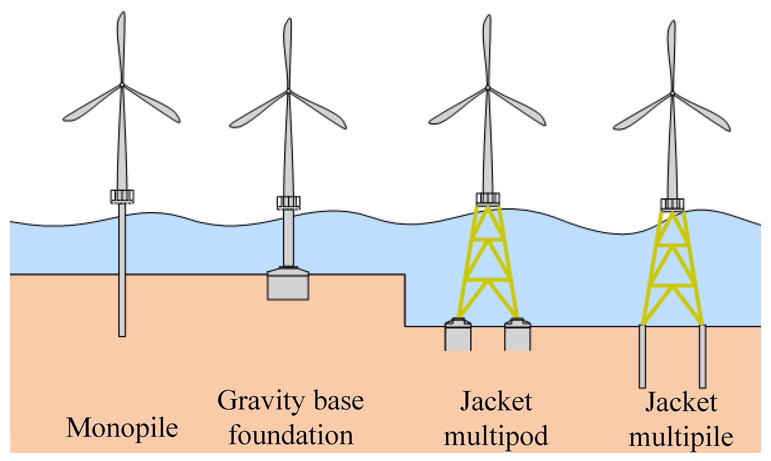
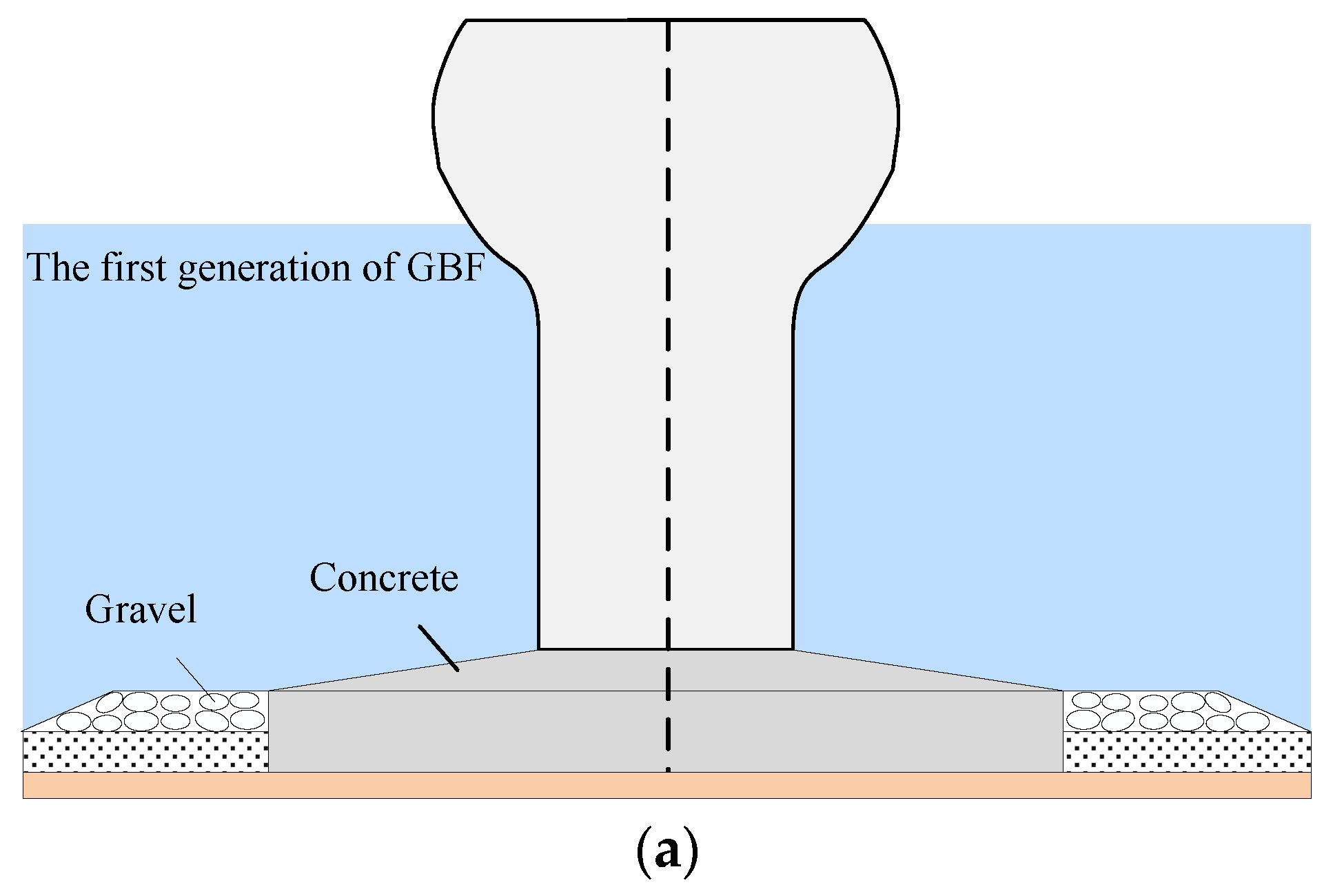
2. Nonlinear Dynamic Analysis of OWT on Gravity Base Foundation

Offshore wind farms gradually move to deeper water areas; thus, offshore wind turbines supported by third-generation GBFs are selected in this study for further analysis. The OWTs consists of three main components, namely the wind turbine tower, the GBF and the foundation bed, as shown in Figure 3.

2.1. Loads on the OWTs

Typical loads acting on the OWTs in the offshore area are wave and wave loads, as shown in Figure 3a. These loads are calculated as follows:

The wind load acting on the OWTs consists of two components, namely the distributed force acting on the tower structure and the thrust force acting on the rotor. The distributed force and the thrust force are mainly determined by the wind velocity. The wind velocity increases with the increases of the distance from the ground surface due to the ground friction force, and it will tend toward a stable state when the distance reaches a certain height. According to the statistical data, the wind speed at any point is a smooth Gaussian random process. It can be divided into the mean wind velocity and fluctuating wind velocity. Then, the distributed force acting on the tower structure can be calculated as follows [37]:

$$F_i=0.5{\rho }_a{C}_D{D}_i{h}_i\left[V_m\left(z,t\right)+V_u\left(z,t\right)\right]$$

(1)

where F_i is the wind force on the beam segment i of the OWTs above the mean sea level, ρ_a is the air density, C_D is the drag coefficient, D_i and h_i are the diameter and length of the beam segment i, and V_m(z,t) and V_u(z,t) are the mean wind velocity and fluctuating wind velocity at height z, respectively.

The thrust force acting on the rotor can be calculated by Bernouli’s equation [38], given as

$$F_T=0.5{\rho }_a\pi C_T{R}_T^2{V}_m^2\left(z_R,t\right)\left[1+2V_u\left(z_R,t\right)/V_m\left(z_R,t\right)\right]$$

(2)

where C_T is the thrust coefficient, R_T is the rotor radius, and $V_m\left(z_R,t\right)$ and $V_u\left(z_R,t\right)$ are the mean wind velocity and fluctuating wind velocity at the hub height of the rotor, respectively.

Morison’s equation is usually suggested to calculate the wave load acting on the offshore structure [17]. According to Morison’s equation, the wave force F_w acting on the OWT can be divided into two parts: the drag force F_D proportional to the square of the instantaneous flow velocity and the inertia force F_I in phase with the local flow acceleration [39]. The drag force is proposed based on the steady flow theory, while the inertia force is proposed based on the potential flow theory, given as

$$F_{wi}=F_{Di}+F_{Ii}=0.5{\rho }_w{C}_D{D}_i{V}_x(z,t)\left|V_x(z,t)\right|dz+0.25\pi {\rho }_w{C}_M{D}_i^2\frac{\partial V_x(z,t)}{\partial t}dz$$

(3)

where F_wi, F_Di and F_Ii are the wave force, drag force and inertia force acting on the segment i of the OWTs below the mean sea level, respectively; C_M is the inertia coefficient; ρ_w is the water density; V_x(z,t) is the wave velocity in the x direction [36].

It should be noted that there is also an additional hydrodynamic pressure on the structure due to the dynamic excitation, which may change the dynamic characteristics of the OWTs [40]. This action between OWTs and water can be simulated by the hydraulic added mass, as follows [41,42]:

$$m_a=0.25\pi D_i^2{C}_a{\rho }_w$$

(4)

where C_a is the added mass coefficient.

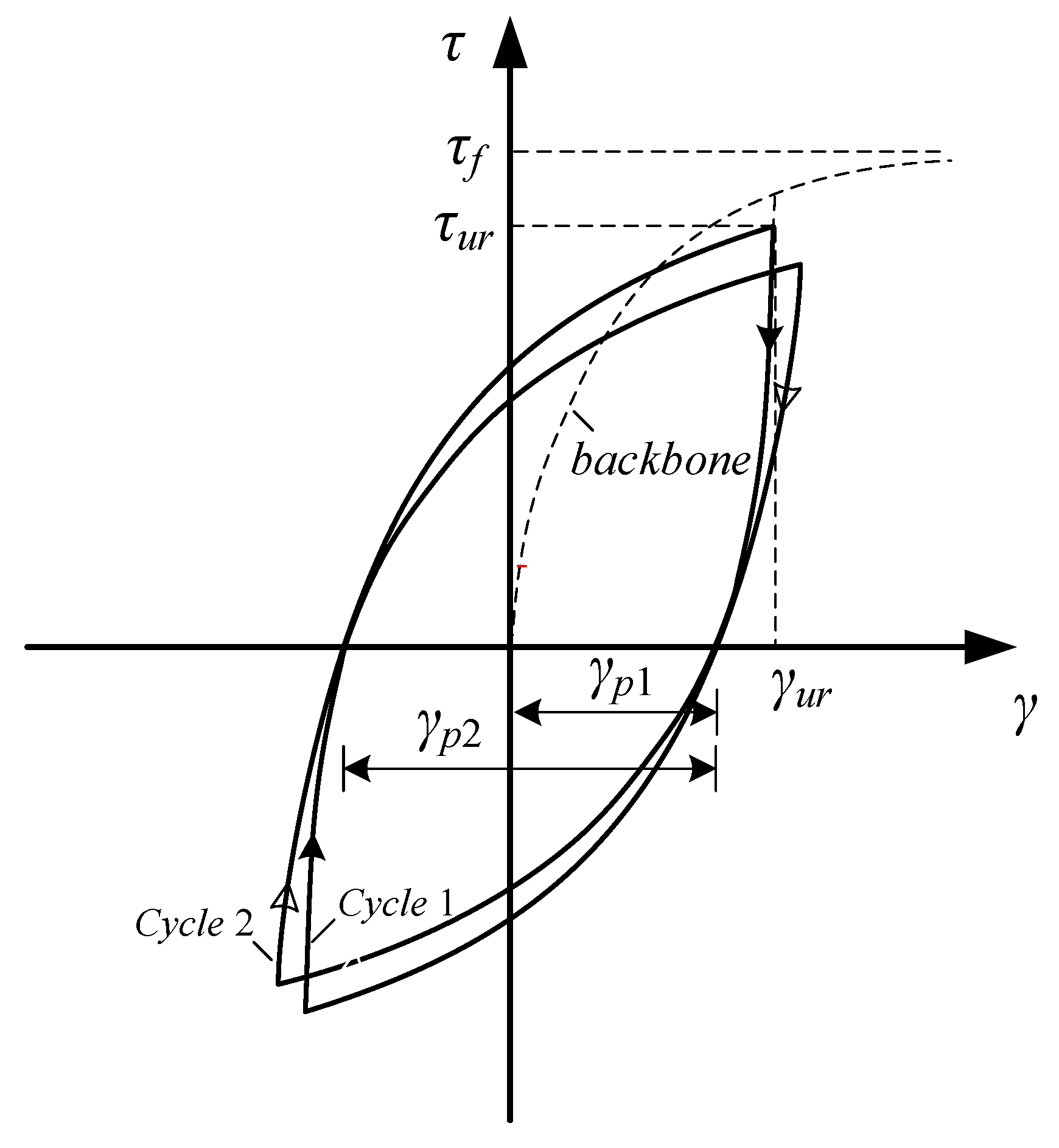
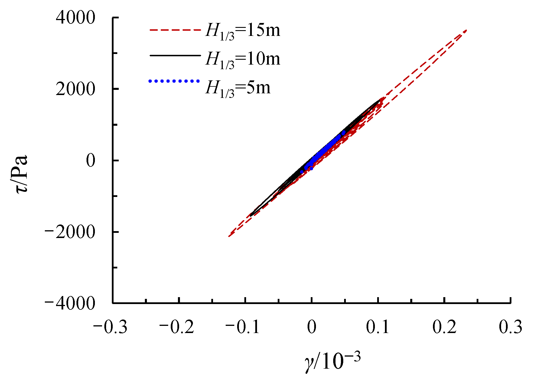
2.2. Nonlinear Interaction between Soil and GBF

It is obvious that dynamic nonlinear characteristics will be generated between the soil and GBF when the OWTs is subjected to the combination of wind and wave loading. Here, the nonlinear dynamic Winkler foundation model is used to simulate the nonlinear interaction between the soil and GBF. It is of vital importance for the dynamic Winkler model to capture the features of soil surrounding the GBF, including the soil nonlinearity, the soil stiffness and strength degradation. For a typical OWT supported on the GBF, the soil around the GBF is a backfill layer consisting of sandy soils, as shown in Figure 3. For a foundation embedded in sandy soil, there is usually no gapping between the soil and the foundation when it is subjected to a dynamic load [43]. Then, hyperbolic shear stress-strain curves with Masing’s rule are used to account for the nonlinear interaction between sandy soil and the foundation as suggested by Hardin and Drnevich [44]. In order to consider the cyclic degradation or hardening behaviors of soil, the modified Pyke’s factor is integrated into the Hardin–Drnevich model [45,46], as shown in Figure 4. Then, the hysteretic curve of shear stress–strain can be expressed as

$$\tau \pm {\tau }_{ur}=\frac{\gamma \pm {\gamma }_{ur}}{1/{\delta }_G{G}_0+\left|\gamma -{\gamma }_{ur}\right|/({\kappa }_0{\tau }_f)}$$

(5)

$${\kappa }_0=1\pm \frac{{\tau }_{ur}}{{\delta }_q{\tau }_f}$$

(6)

where G₀ is the initial shear modulus of soil, γ and τ are the shear strain and shear stress of soil at the current state, γ_ur and τ_ur are the current shear strain and stress of soil at the beginning of unloading or reloading, respectively, κ₀ is the modified Pyke’s factor, and signs of ‘+’ and ‘−’ represent the unloading and reloading process, respectively. δ_G and δ_q are the shear modulus and strength degradation (or hardening) factors of the soil, given as [47]

$${\delta }_G={\delta }_{GN}+(1-{\delta }_{GN})e^{-b{\gamma }_p}$$

(7)

$${\delta }_q={\delta }_{qN}+(1-{\delta }_{qN})e^{-b{\gamma }_p}$$

(8)

where δ_GN and δ_qN are the residual stiffness and residual strength ratio, b is a constant reflecting the degradation or hardening rate of the accumulative shear strain, γ_p is the accumulated plastic shear strain, which is calculated by the sum of the plastic shear strain developed at each load cycle, given as

$${\gamma }_p={\displaystyle \sum {\gamma }_{pi}} (i=1, 2, 3, \cdots 2N-1, 2N)$$

(9)

where N is the number of stress–strain hysteresis loops or load cycles. Neither the combined wind and wave seismic loads nor the dynamic response of the OWTs under the combined loads are symmetrical cycles. Here, the number of reloading and unloading at the current time step is used to determine the plastic shear strain of the soil at each cycle.

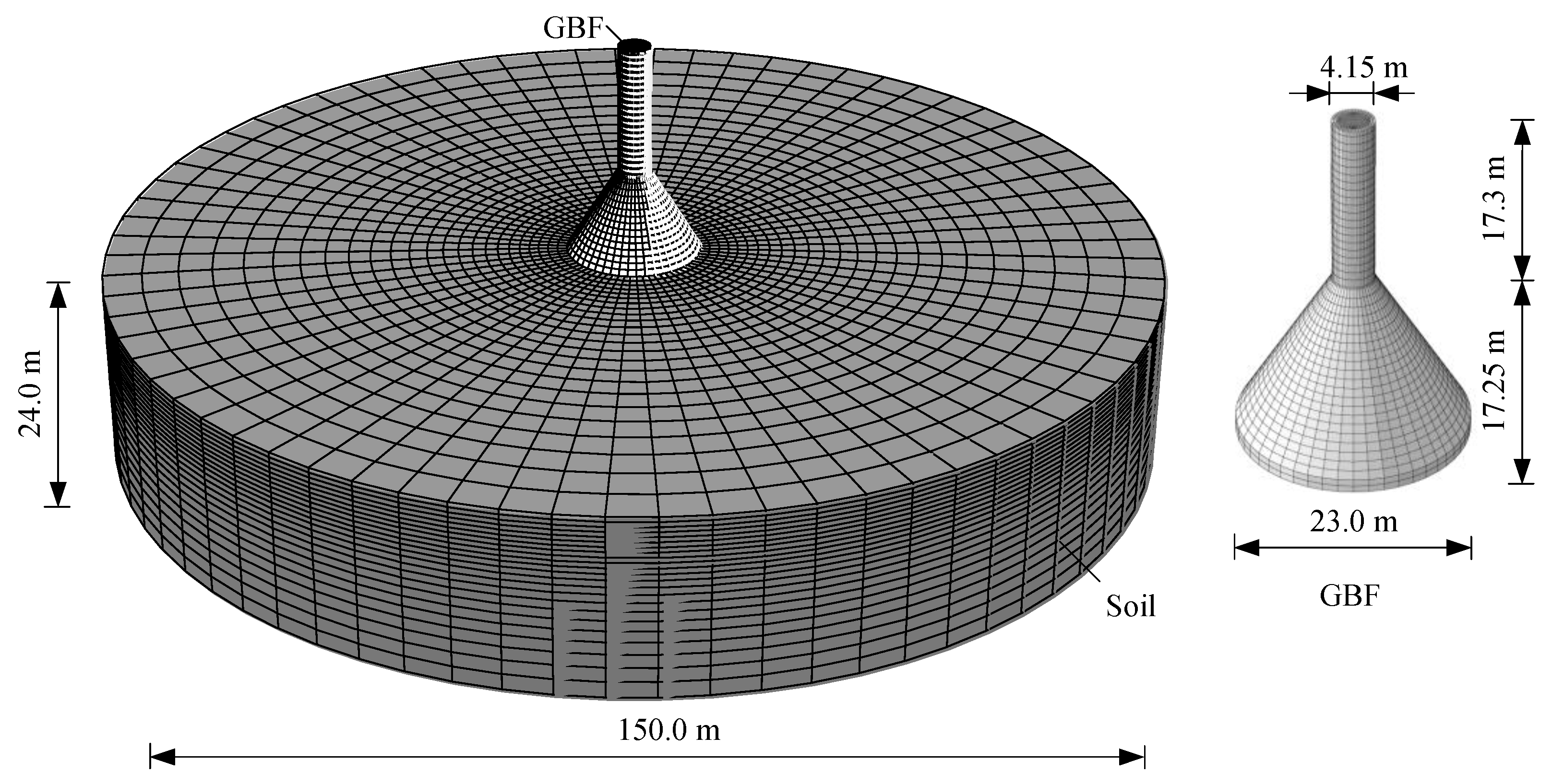
2.3. Analysis Model for the OWT on the GBF

To obtain the dynamic response of the OWT on the GBF, the tower is discretized into n segments, which are modeled as a continuous elastic beam based on the displacement and force coordination of the beam nodes. The mass density is assembled to the nodes of the beam to account for the inertia characteristics of the tower [48,49], as shown in Figure 3b. In addition, to achieve higher accuracy, the cross-sectional inhomogeneity of the tower is considered here by setting different diameters and thicknesses of the beam segments. It should be noted that the rotor nacelle assembly (RNA, includes the rotor, nacelle and blades) may also affect the performance of the wind turbine [29,30]. Considering the nonlinear interaction between GBF and the soil and analyzing the dynamic response of the OWTs under wind and wave loads are the main focuses of this study. The effect of the RNA on the dynamic response of the OWTs is not taken into account. Therefore, the RNA is assumed to be a concentrated mass at the top of the tower and is considered as rigidly connected to the tower beam segment.

Similarity, the lateral distributed load can be simplified as the concentrated force acted on the node, and [F_i] is a two-dimensional load vector acting on the node i containing concentrated force and moment. The GBF can be considered as a rigid caisson foundation [18,24,25]. Then, the horizontal-rocking vibration equilibrium equation of the whole OWTs with respect to the bottom of the tower structure can be given as

$$\mathbf{M}\mathsf{ü}+\mathbf{C}\mathsf{ü}+\mathbf{Ku}=\mathbf{F}$$

(10)

where u and F are the dynamic displacement and force matrices of the OWTs, and M, C, and K are the mass matrix, damping matrix and stiffness matrix of the OWTs, respectively.

The mass, damping and stiffness of the wind turbine tower are easy to determine as it is an elastic material. The key to obtaining the dynamic response of the OWTs is to determine the dynamic characteristics of the GBF. The GBF was considered as a surface foundation in previous studies [18,25]. Actually, the GBF is an irregularly shaped partially embedded foundation in engineering practice, and treating it as a surface foundation will lead to inaccurate results in the dynamic response of the GBF. According to the conditions of force equilibrium, the dynamic equation of a partially embedded foundation can be written as

$${\mathbf{M}}_g\left\{\begin{array}{c}{\ddot{u}}_g\\ {\ddot{\theta }}_g\end{array}\right\}+{\mathbf{C}}_g\left\{\begin{array}{c}{\dot{u}}_g\\ {\dot{\theta }}_g\end{array}\right\}+{\mathbf{K}}_g\left\{\begin{array}{c}{u}_g\\ {\theta }_g\end{array}\right\}=\left\{\begin{array}{c}{H}_G\\ M_G\end{array}\right\}$$

(11)

where M_g, K_g and C_g are the mass matrix, the dynamic stiffness matrix and the damping matrix of the GBF, respectively; u_g and θ_g are the lateral displacements and the rocking angel of the base of the GBF; H_G and M_G are the dynamic horizontal and moment load acting on the top of the GBF.

Based on the dynamic Winkler theory, the dynamic characteristics of a massless partially embedded foundation can be determined by the soil properties at the base of the foundation and the soil properties on the side of the embedded part of the foundation. Considering the embedded depth is usually small, the embedded part of the foundation can be treated as a cylindrical structure; then, the stiffness and damping matrices of the GBF can be calculated as

$${\mathbf{K}}_g=\left[\begin{array}{cc}{K}_{hh}& K_{hr}\\ K_{rh}& K_{rr}\end{array}\right]=\left[\begin{array}{cc}{K}_h+k_{h}d& \frac{1}{2}{k}_h{d}^2\\ \frac{1}{2}{k}_h{d}^2& K_r+\frac{1}{3}{k}_h{d}^3+k_{r}d\end{array}\right]$$

(12)

$${\mathbf{C}}_g=\left[\begin{array}{cc}{C}_{hh}& C_{hr}\\ C_{rh}& C_{rr}\end{array}\right]=\left[\begin{array}{cc}{C}_h+c_{h}d& \frac{1}{2}{c}_h{d}^2\\ \frac{1}{2}{c}_h{d}^2& C_r+\frac{1}{3}{c}_h{d}^3+c_{r}d\end{array}\right]$$

(13)

where d is the embedded depth of the GBF; k_h, c_h and k_r, c_r are the horizontal and rocking stiffness and damping of the spring simulating the soil properties around the GBF, respectively; K_h, C_h and K_r, C_r are the horizontal, rocking stiffness and damping of the spring at the base of GBF, which can be calculated by the stiffness and damping of the rigid circular surface foundation [50].

The matrix M_g can be determined by the geometric parameters and the mass of the GBF m_g, given as

$${\mathbf{M}}_g=\left[\begin{array}{cc}{m}_g& m_g{L}_0\\ m_g{L}_0& J_g+m_g{L}_0\end{array}\right]$$

(14)

where J_g is the inertia moment of the GBF, and L₀ is the height from the bottom of the GBF to the center of gravity of the GBF.

Integrating Equation (10) and the dynamic equilibrium equation of the wind turbine tower structure, and according to the displacement and force coordination conditions of node n + 1 (see Figure 3), the dynamic matrices M, C and K of the whole OWTs can be established, which can be found in Appendix A. It is obvious that all the stiffness or damping coefficients mentioned in Equations (12) and (13) are closely related to the shear modulus of soil, and the current state of the shear modulus of the soil must be determined by an iterative method due to the effect of soil nonlinearity. As long as the soil parameters are determined, such as the initial shear modulus, effective friction angle, and Poisson’s ratio of soil, the dynamic response of the whole OWTs can be obtained by solving the dynamic equilibrium equation through the Newmark-β method with the linear acceleration method [51]. The flow chart for the nonlinear analysis is illustrated in Figure 5.

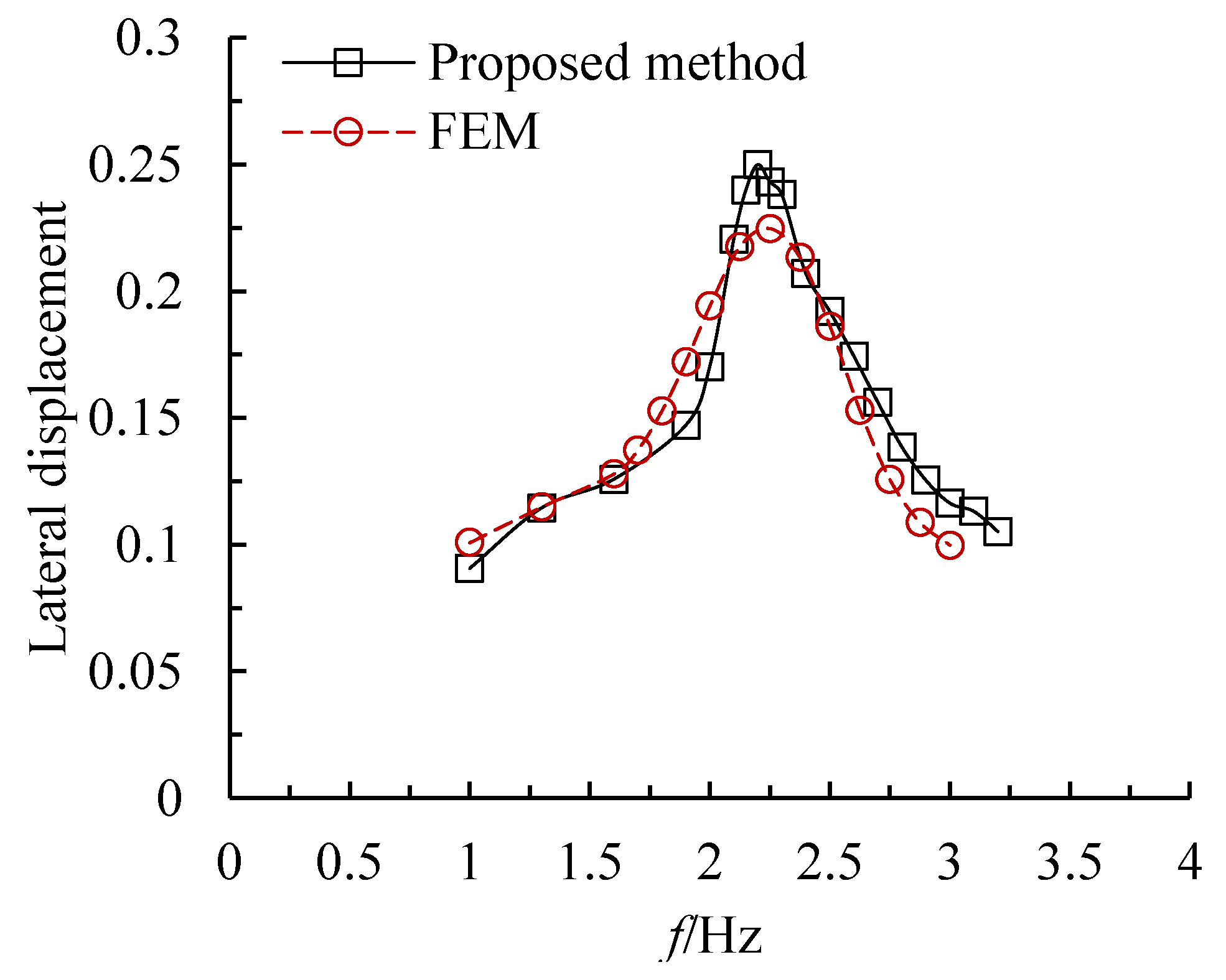
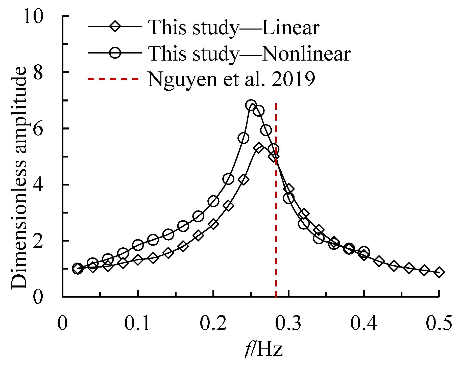
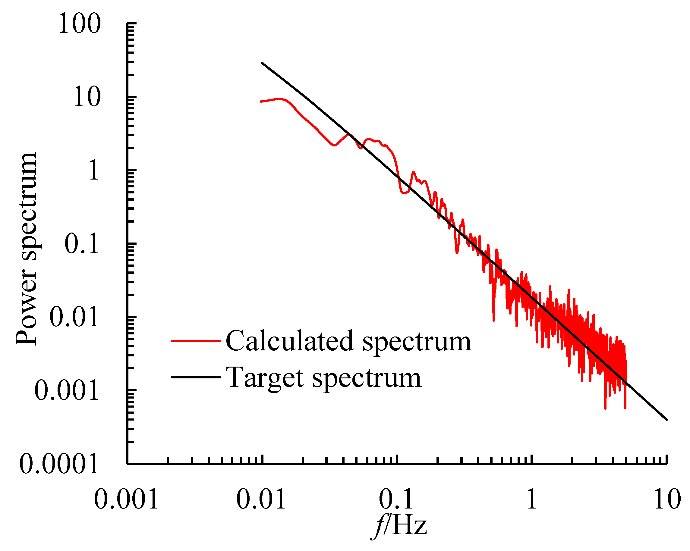
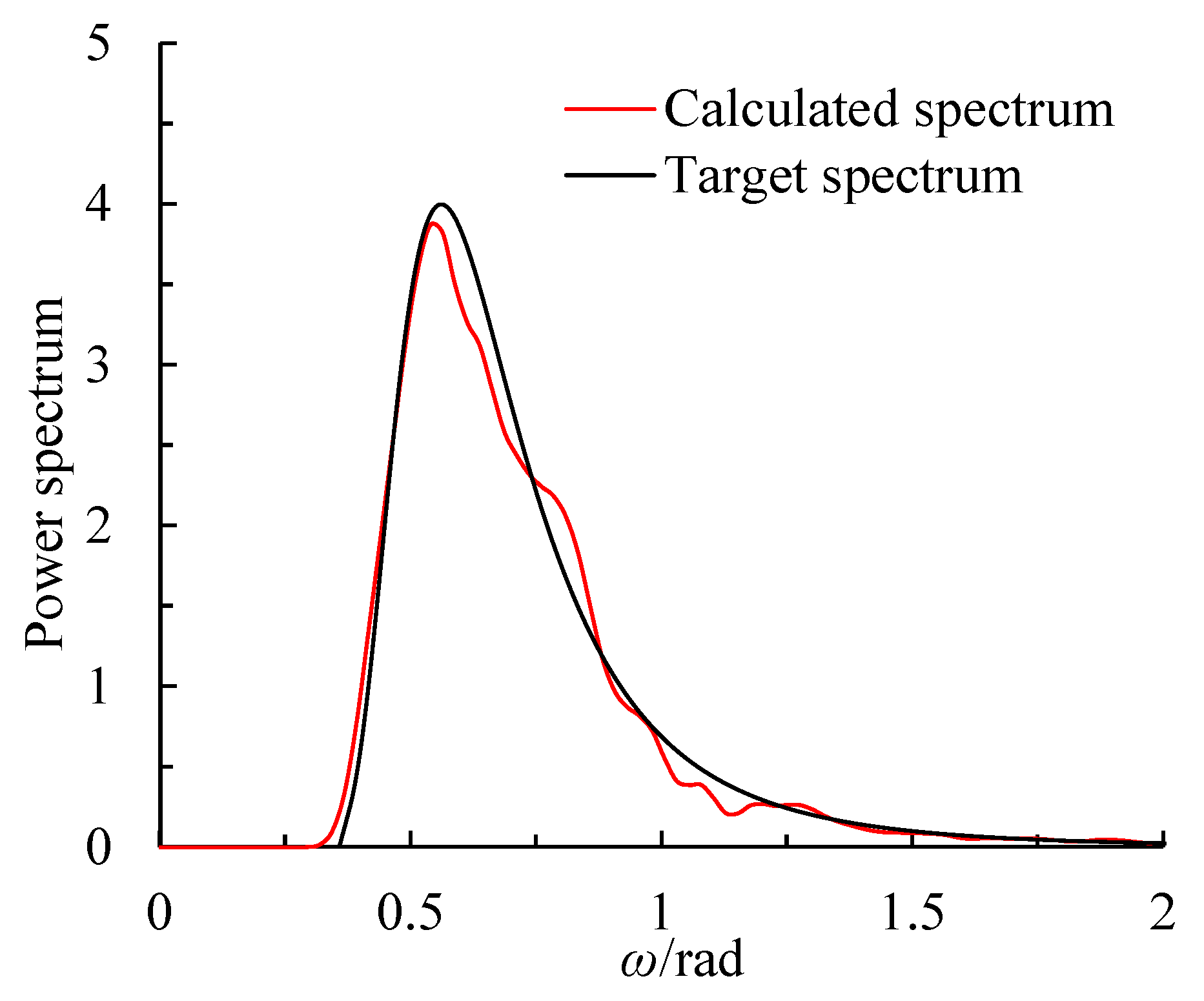
3. Verification of the Proposed Method

A thorough review of the literature available on third-generation GBFs shows that experimental and theoretical data on lateral dynamic response are relatively scarce, especially considering the effect of the soil nonlinearity. Therefore, the proposed analysis method is verified by the lateral characteristics of the OWT on GBF by the FEM method. The OWTs of 3 MW at Hankyung II Wind Park was selected as a target structure, and the geometry of the OWTs used in this paper can be found in Nguyen et al. [24], as illustrated in Figure 5. The mass of the rotor nacelle assembly is 94,600 kg. The top and bottom diameters of the wind turbine tower are 2.32 m and 4.15 m, and the thickness of the section varies with the elevation of the tower. The geometrical details of the wind turbine tower are listed in

Table 1. Parameters of the wind turbine tower [24].

Height (m)	Thickness (mm)	Height (m)	Thickness (mm)
0~5.4	40	42.2~50.9	21
5.4~21.9	26	50.9~53.8	19
21.9~30.6	24	53.8~56.7	18
30.6~36.4	23	56.7~59.6	17
36.4~42.2	22	59.6~77.3	16

, and the mechanical properties of soil are listed in

Table 2. Material properties of the OWT on the GBF [24].

	Material Property	Elastic Modulus E MPa	Poisson’s Ratio ν	Density ρ kg/m3
Tower	Steel	210,000	0.3	7698
GBF	Concrete	33,500	0.2	2500
	Infill sand	66.5	0.325	1620
Foundation bed	Scour protection layer	/	/	1800
	Backfill layer	66.5	0.325	1620
	Gravel layer	140	0.3	1500
	Filter layer	140	0.3	2100
Ground	Sand layer	66.5	0.325	1620

.

The reliability of the simplified method when considering soil nonlinearity should be analyzed. The nonlinear characteristics occur only in the interaction between soil and foundation. For simplicity, the nonlinear time domain dynamic analysis model of a laterally loaded foundation is developed by the finite element method to verify the validity of the proposed method. Here, the dimensions of the GBF illustrated in Figure 6 are used, and the finite element mesh of the GBF is depicted in Figure 7. The soil filling and surrounding the GBF is in accordance with the Mohr-Column model. The Young’s modulus, Poisson’s ratio, mass density and effective internal friction angle of the soil are 66.5 MPa, 0.325, 1620 kg/m³ and 30°, respectively. The damping properties of soil are simulated by using Rayleigh damping coefficients, and the value of the first mode and fifth mode natural frequencies of soil are used to define the Rayleigh damping coefficients as α = 0.4073 and β = 0.00614 [52,53]. The viscoelastic boundary is used in this paper for attenuating the wave reflection in the dynamic finite element analysis. Slippage and gapping between the soil and GBF are not allowed during the analysis.

Figure 8 shows the dynamic lateral displacement atop the caisson as a function of the frequency f under a 20 MN harmonic horizontal load atop the GBF. The proposed simplified method predicts slightly smaller values in the low frequency range and slightly larger values in the medium and high frequency range than those by the FEM. The resonant frequencies of the GBF calculated by the proposed method and FEM are 2.5 Hz and 2.25 Hz, and these two values are very close, which verifies the rationality of the simplified method. The difference between the FEM and proposed method may be attributed to the rigidity assumptions of the GBF. The time histories of displacement at the top center of the foundation when f = 2.25 Hz are extracted to make a further comparison, as shown in Figure 9. The results show that the time histories of lateral displacement atop the GBF calculated by the proposed method and FEM are in good agreement. Note that both models have slight asymmetry at the first several cycles, while the are more uniform at the subsequent loading cycles. This is mainly due to the soil nonlinearity developed during the first loading half-cycle, which is similar to the results in Huang et al. [54].

On the other hand, resonant frequencies and mode shapes are important properties for studying the dynamic characteristics of wind turbines. Therefore, the dynamic responses of the OWTs at different frequencies calculated by the present method are shown in Figure 10. The lateral load is a 100 kN sinusoidal load, whose magnitude is close to the combined wind and wave load. The lateral dynamic displacement is normalized by the displacement under static response. As shown in Figure 10, the resonant frequency of the OWTs is 0.26 Hz without considering the nonlinear interaction between the GBF and soil, which is almost equal to the 0.283 Hz obtained by the finite element method [24]. This comparison also ensures the reliability of the present simplified method for elastic analysis. The resonant frequency of the OWTs is about 0.25 Hz when considering the nonlinear interaction between the GBF and soil. Obviously, the effect of soil nonlinearity will result in an increase in the amplitude of the dynamic response of the OWTs and a decrease in the resonant frequency of the OWTs.

4. Performance of OWTs under Wind and Wave Loads

The OWTs in Section 3 is subsequently selected to further investigate the effects of the combined load on the dynamic response.

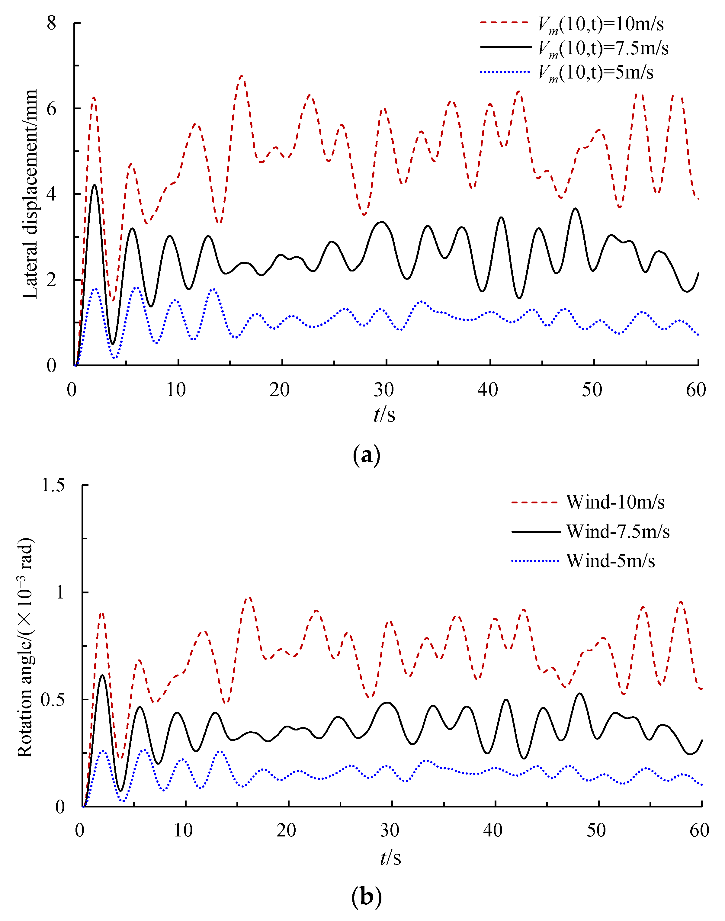
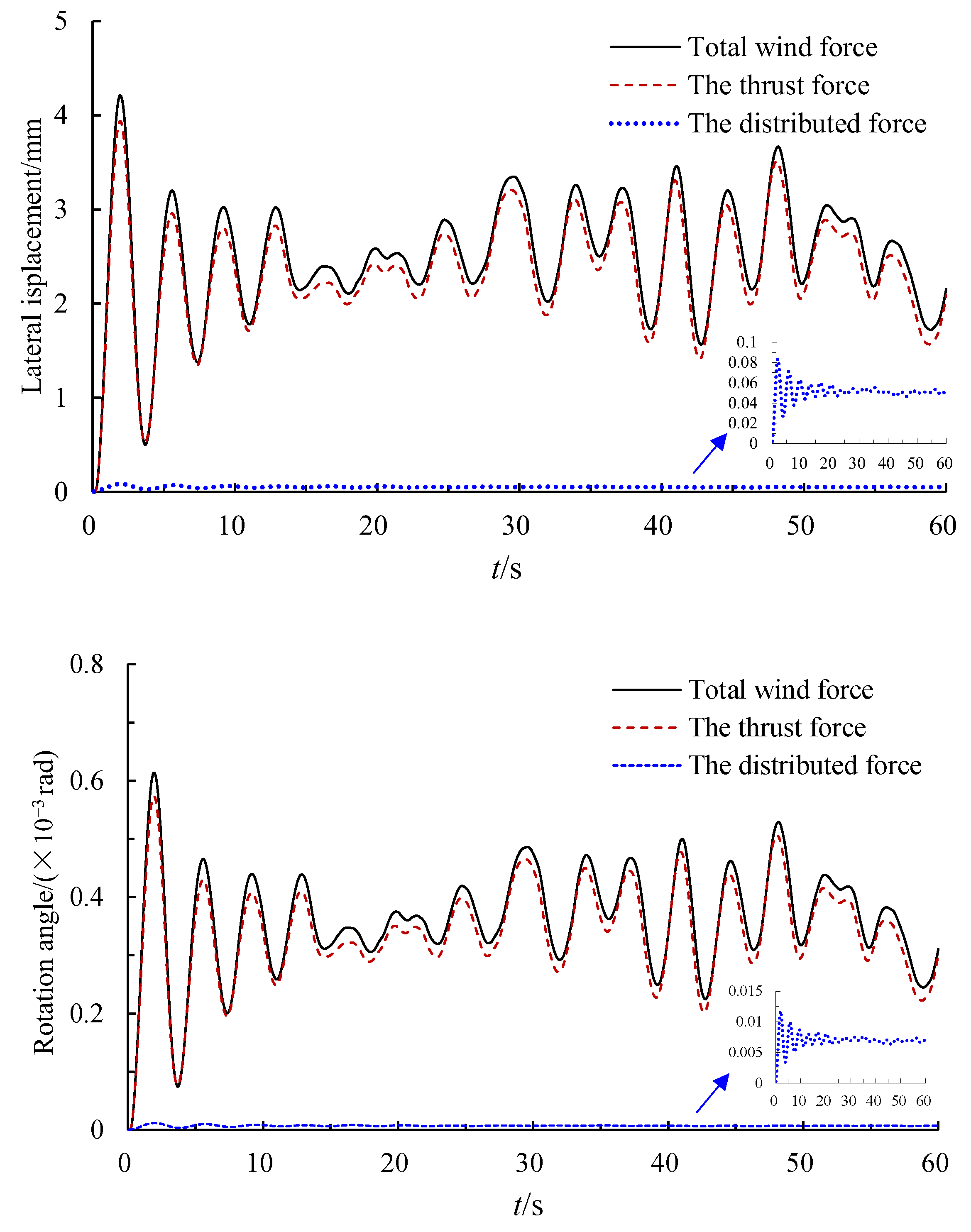
4.1. Response to the Wind Loads

The wind loads can be divided into the distributed force and the thrust force. The key to calculating the values of the distributed force and the thrust force is to determine the wind velocity.

The logarithmic model is used to calculate the mean wind velocity, given as [55]

$$V_m\left(z,t\right)=V_m\left(10,t\right)\frac{\ln (z/z_0)}{\ln (10/z_0)}$$

(15)

where z₀ is the roughness length, taken as 0.003, and $V_m\left(10,t\right)$ is the mean wind velocity at the height of 10 m.

The Kaimal wind speed spectrum is selected to simulate fluctuating wind velocity, as suggested in the IEC standard [56,57]. The Kaimal spectrum introduces a stochastic function related to the height from the ground, given as

$$S\left(f,z\right)=\frac{I^2\left[V_m\left(z,t\right)+V_u\left(z,t\right)\right]L_s}{{\left(1+1.5\frac{f\cdot L_s}{\left[V_m\left(z,t\right)+V_u\left(z,t\right)\right]}\right)}^{5/3}}$$

(16)

where I is the turbulence intensity, given as 0.11, and f and L_s are the frequency and length scale.

Then, $V_m\left(10,t\right)$ = 7.5 m/s is selected to calculate the wind loads acting on the wind turbine. As suggested by Liang et al. [17] and Cheng et al. [36], ρ_a can be assumed as 1.225, and C_D and C_T are taken as 1.2 and 1.0, respectively. The power spectrum of wind load when $V_m\left(10,t\right)$ = 7.5 m/s is given in Figure 11, which shows a good agreement with the target spectrum; the time history of the wind load acting at the hub of the OWTs when $V_m\left(10,t\right)$ = 7.5 m/s is illustrated in Figure 12.

In order to analyze the wind load effect on the dynamic response of the OWTs, three mean wind velocities at a height of 10 m, $V_m\left(10,t\right)$ = 5 m/s, 7.5 m/s and 10 m/s, are used to calculate the mean wind velocity in this study. Figure 13 demonstrates the lateral displacement and rocking angle atop the GBF when experiencing the wind loads only. The results show that the peak displacement of the GBF increases significantly with the increase of the mean wind velocity $V_m\left(10,t\right)$, and there is a large increment of lateral displacement occurring at the beginning of the wind loading stage. This is mainly attributed to the fact that the wind load is an asymmetric load, which results in the accumulation of displacement in the horizontal direction. This finding is also similar to the results reported by Cheng et al. [36] in terms of the effect of environmental loads on the suction foundation. This phenomenon also can be found in the soil stress–strain hysteresis curves at 0.5 m from the soil surface given in Figure 14.

As seen in Figure 14, the backbone curves of stress–strain hysteresis curves at different mean wind velocities are partially overlapping, and the strain accumulation in horizontal direction and hysteresis loops areas after each cycle increase with the increase of the wind velocity. This stems from the fact that the wind load is greater when $V_m\left(10,t\right)$ = 10 m/s compared to $V_m\left(10,t\right)$ = 7.5 m/s and 5 m/s, resulting in the soil showing a stronger nonlinearity. This is also the main reason that the displacement of the GBF shows a nonlinear increase trend under different mean wind velocity $V_m\left(10,t\right)$. In order to further analyze the thrust force and the distributed force generated by the wind on the dynamic response of the OWTs, the time histories of lateral displacement and rotation angle of the GBF when $V_m\left(10,t\right)$ = 7.5 m/s are also illustrated in Figure 15. The results show that the thrust force acting on the rotor plays an important role in the dynamic response of the GBF, while the distributed wind load has little effect on the dynamic response of the foundation.

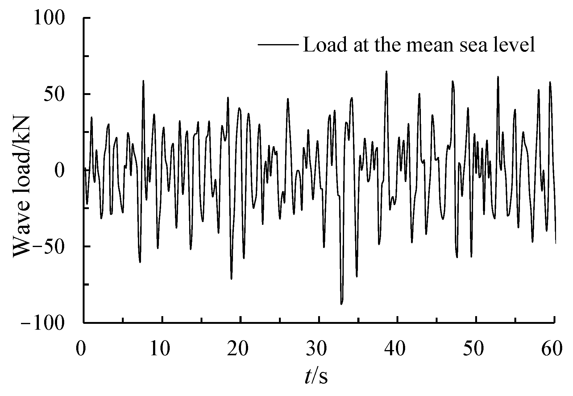
4.2. Response to the Wave Loads

Likewise, the key to calculating the values of the drag force F_D and the inertia force F_I is to determine the wave velocity V_x(z,t), the inertia coefficient C_M and the drag coefficient C_D, as shown in Equation (3). As suggested by Liang et al. [17], C_M and C_D can be taken as 2.0 and 1.2, respectively. Stochastic wave theory was adopted by using the Pierson and Moskowitz (P–M) spectrum to simulate the wave velocity V_x(z,t) acting on the OWTs [36,58]. The P–M spectrum is a special case of a much wider class termed the gamma-spectra, which can be introduced in close formal analogy with the generalized gamma probability distribution. It can easily describe the peculiar characteristics of wind waves, generated over a long period of time. The P–M spectrum is given as

$$S\left(\omega \right)=0.75{\omega }^{-5}\exp \left(-3.11{\omega }^{-4}{H}_{1/3}^{-2}\right)$$

(17)

where H_1/3 and ω are the significant wave height and the circular frequency, respectively.

To determine the amplitude of the wave load, the significant wave height H_1/3 should be determined first. Then, the significant wave height H_1/3 = 10 m is selected to calculate the wave loads on the GBF, and the wind structure below the mean sea level is divided into five segments. The power spectral density with the target spectrum is given in Figure 16. The results also show that the calculated spectrum is in good agreement with the target spectrum. The time history of the wave load acting at the mean sea level when H_1/3 = 10 m is illustrated in Figure 17.

In order to obtain the wave load effect on the dynamic response of the OWTs, the significant wave heights of H_1/3 = 5 m, 10 m and 15 m are selected to calculate the wind load on the OWTs in this study. The time histories of the lateral displacement and rocking angle atop the GBF when experiencing the wave loads only are shown in Figure 18. It is obvious that the displacement of the GBF increases with the increase of the significant wave height H_1/3. The most important reason is the increase in wave force due to the increase in H_1/3. Meanwhile, the increase in soil nonlinearity is also one of the reasons for the increase in displacement response. This can be explained by the stress –strain hysteresis curves of soil around the GBF, as depicted in Figure 19. Although the soil strain is relatively small, it can still be seen that the hysteresis loop area is increasing with the increase of the H_1/3.

In order to further analyze the drag force F_D and the inertia force F_I on the dynamic response of the OWTs, the time histories of lateral displacement and rotation angle atop the GBF when H_1/3 = 10 are shown in Figure 20. The results show that the dynamic displacement of the GBF caused by the drag force F_D is smaller than that of the GBF caused by the inertia force F_I. However, the maximum dynamic displacement of the GBF caused by the drag force F_D is almost the same as that of the GBF caused by the inertia force F_I.

4.3. Response to the Combined Loads

In order to investigate the dynamic response of the OWTs subjected to the combined wind and wave loads, the mean wind velocity $V_m\left(10,t\right)$ = 7.5 m/s and three different significant wave heights, H_1/3 = 5 m, 10 m and 15 m, are also selected to analyze the effect of the combined wind and loads on the dynamic response of the GBF. The time histories of dynamic response atop the GBF are illustrated in Figure 21. Since the wave loads are relatively small compared to the wind loads, the time history curves of the dynamic response of the GBF under combined wind and wave loads show a similar trend to that of the dynamic response of the GBF under the wind loads only. Figure 22 gives the stress–strain curves of soil around the GBF. It is obvious that the degree of soil nonlinearity increases with the increase of the H_1/3. Compared to the results in Figure 14, it can also be found that the hysteresis loop areas increase significantly when the wave load is taken into account.

In the meantime, the mean wind velocity $V_m\left(10,t\right)$ = 7.5 m/s and the significant wave height H_1/3 = 10 m are selected to calculate the wind and wave loads on the OWTs in this study. The time histories of dynamic response atop the GBF under combined wind and wave loads are shown in Figure 23. The results show that there is an overall increase in the time history curves of the lateral displacement and rotation angle atop the GBF under wind load compared to that of the lateral displacement and rotation angle atop the GBF under wind load only. It can also be seen that the time history curves of the lateral displacement and rotation angle atop the GBF under the wind loads only oscillate more smoothly than that of the lateral displacement and rotation angle atop the GBF under the combined wind and wave loads.

5. Summary and Conclusions

In this study, a simplified dynamic Winkler model was proposed to analyze the lateral dynamic response of the offshore wind turbine on GBF, in which the nonlinear behavior of the GBF and soil was considered. The results and numerical analyses were compared. Then, the wind and wave load on the dynamic responses of the OWTs were also investigated. The following conclusions can be drawn:

(1)

A nonlinear dynamic analysis model for the offshore wind turbine supported on GBF was proposed, in which the GBF is simplified as a rigid foundation and the wind turbine tower is simulated as a structure composed of several elastic beams. The proposed time domain method considering soil nonlinearity provides a good estimation of the time history of the dynamic response of the OWT supported on the GBF.

(2)

The peak displacement of the GBF increases significantly with the increase of the mean wind velocity $V_m\left(10,t\right)$. It can be found that a large increment of displacement in the horizontal direction will occur at the beginning of the loading stage when the OWT supported on the GBF is subjected to the wind load, and the lateral dynamic responses of the GBF are more affected by the thrust force acting on the structure than by the distributed load.

(3)

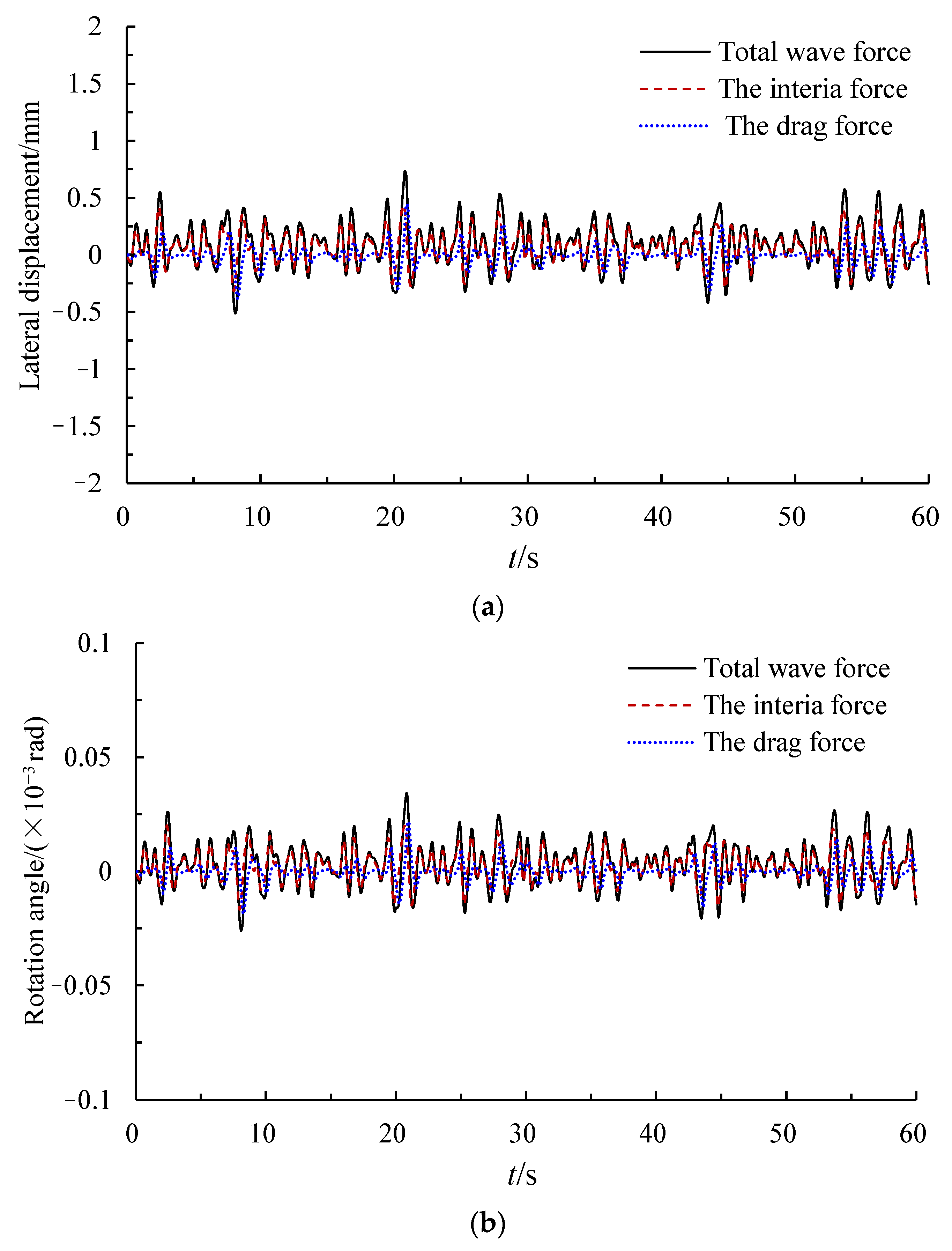
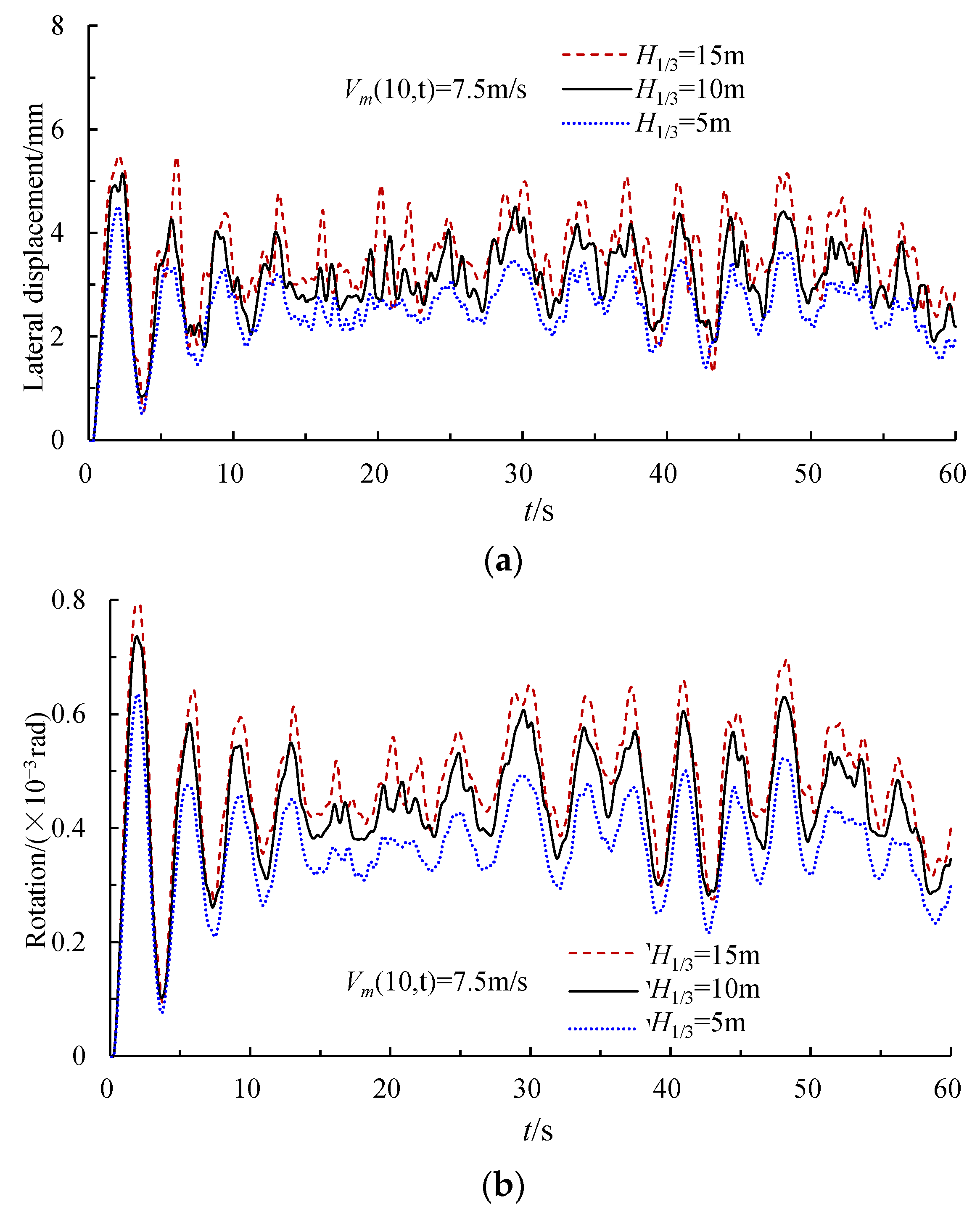
The significant wave height H_1/3 is the main factor in determining the dynamic response of the OWTs supported on a GBF under wave loading. The dynamic response of the GBF increases as the H_1/3 increases, and the dynamic response of the GBF caused by the drag force is smaller than that of the GBF caused by the inertia force when H_1/3 is the same. However, the maximum dynamic displacement of the GBF caused by the drag force is almost the same as that of the GBF caused by the inertia force.

(4)

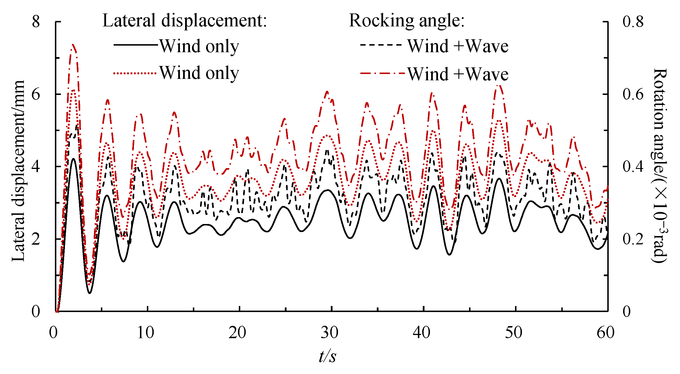
The time history curves of the dynamic response of the GBF under combined wind and wave loads show a similar trend to that of the dynamic response of the GBF under the wind loads only. However, the time history curves of the lateral displacement and rotation angle atop the GBF under the wind loads only oscillate more smoothly than that of the lateral displacement and rotation angle atop the GBF under the combined wind and wave loads.

References

1. Wu, X.; Hu, Y.; Li, Y.; Jian, Y.; Duan, L.; Wang, T.H.; Adcock, T.; Jiang, Z.Y.; Gao, Z.; Lin, Z.L.; et al. Foundations of offshore wind turbines: A review. Renew. Sustain. Energy Rev. 2019, 104, 379–393. [Google Scholar] [CrossRef] [Green Version]
2. Cai, X.; Yang, R.X.; Zhou, J.Q.; Fang, Z.X.; Yang, M.Y.; Shi, X.Q.; Chen, Q. Review on Offshore Wind Power Integration via DC Transmission. Automa. Electr. Power Syst. 2021, 45, 2–22. (In Chinese) [Google Scholar] [CrossRef]
3. Díaz, H.; Soares, C.G. Review of the current status, technology and future trends of offshore wind farms. Ocean Eng. 2020, 209, 107381. [Google Scholar] [CrossRef]
4. Sun, X.; Huang, D.; Wu, G. The current state of offshore wind energy technology development. Energy 2012, 41, 298–312. [Google Scholar] [CrossRef]
5. European Wind Energy Association. Offshore Wind Market Report: 2021 Edition. Available online: https://www.energy.gov/eere/wind/articles/offshore-wind-market-report-2021-edition-released (accessed on 10 September 2022).
6. Peire, K.; Nonneman, H.; Bosschem, E. Gravity base foundations for the thornton bank offshore wind farm. Terra Aqua 2009, 115, 19–29. [Google Scholar]
7. Schallenberg-Rodríguez, J.; Montesdeoca, N.G. Spatial planning to estimate the offshore wind energy potential in coastal regions and islands. Practical case: The Canary Islands. Energy 2018, 143, 91–103. [Google Scholar] [CrossRef]
8. Tricklebank, A.H.; Magee, B.; Halberstadt, P.H. Concrete towers for onshore and offshore wind farms. Concr. Cent. Surrey 2007, 19, 217. [Google Scholar]
9. Futai, M.M.; Haigh, S.K.; Madabhushi, G.S.P. Comparison of the dynamic responses of monopiles and gravity base foundations for offshore wind turbines in sand using centrifuge modelling. Soil. Found. 2021, 61, 50–63. [Google Scholar] [CrossRef]
10. Esteban, M.D.; López-Gutiérrez, J.S.; Negro, V. Gravity-based foundations in the offshore wind sector. J. Mar. Sci. Eng. 2019, 7, 64. [Google Scholar] [CrossRef] [Green Version]
11. Esteban, M.D.; Couñago, B.; López-Gutiérrez, J.S.; Negroa, V.; Vellisco, F. Gravity based support structures for offshore wind turbine generators: Review of the installation process. Ocean. Eng. 2015, 110, 281–291. [Google Scholar] [CrossRef]
12. Guan, M.K.; Zhang, X.F.; Xiang, X.; Zhang, Q.; Ke, Y.S. Research on the construction technology of offshore wind turbine on gravity base foundation. China Water Transp. 2019, 19, 170–172. (In Chinese) [Google Scholar]
13. Mathern, A.; Von der Haar, C.; Marx, S. Concrete support structures for offshore wind turbines: Current status, challenges, and future trends. Energies 2021, 14, 1995. [Google Scholar] [CrossRef]
14. Koekkoek, R.T. Gravity Base Foundations for Offshore Wind Turbines; Delft University of Technology: Delft, The Netherlands, 2015. [Google Scholar]
15. Vahdatirad, M.J.; Griffiths, D.V.; Andersen, L.V.; Andersen, L.; Sørensen, V. Reliability analysis of a gravity-based foundation for wind turbines: A code-based design assessment. Géotechnique 2014, 64, 635–645. [Google Scholar] [CrossRef]
16. Zachert, H.; Wichtmann, T.; Kudella, P.; Triantafyllidis, T. Inspection of a high-cycle accumulation model for sand based on recalculations of a full-scale test on a gravity base foundation for offshore wind turbines. Comput. Geotech. 2020, 126, 103727. [Google Scholar] [CrossRef]
17. Liang, F.Y.; Yuan, Z.C.; Liang, X.; Zhang, H. Seismic response of monopile-supported offshore wind turbines under combined wind, wave and hydrodynamic loads at scoured sites. Comput. Geotech. 2022, 144, 104640. [Google Scholar] [CrossRef]
18. He, R.; Wang, L. Elastic rocking vibration of an offshore Gravity Base Foundation. Appl. Ocean. Res. 2016, 55, 48–58. [Google Scholar] [CrossRef]
19. Yu, L.; Wang, L.Z.; Guo, Z.; Bhattacharya, S.; Nikitas, G.; Li, L.-L.; Xing, Y.-L. Long-term dynamic behavior of monopile supported offshore wind turbines in sand. Theor. Appl. Mech. Lett. 2015, 5, 80–84. [Google Scholar] [CrossRef] [Green Version]
20. Witcher, D. Seismic analysis of wind turbines in the time domain. Wind Energy 2005, 8, 81–91. [Google Scholar] [CrossRef]
21. Lian, J.J.; Yan, X.; Wang, H.J. Dynamic characteristic analysis of new type gravity infrastructure for offshore wind turbine. Acta Energy Sol. Sin. 2016, 37, 1624–1630. (In Chinese) [Google Scholar]
22. Li, Y.; Ong, M.C.; Tang, T. Numerical analysis of wave-induced poro-elastic seabed response around a hexagonal gravity-based offshore foundation. Coast. Eng. 2018, 136, 81–95. [Google Scholar] [CrossRef]
23. Cui, L.; Jeng, D.S.; Liu, J. Numerical analysis of the seabed liquefaction around a fixed gravity-based structure (GBS) of an offshore platform and protection. Ocean Eng. 2022, 249, 110844. [Google Scholar] [CrossRef]
24. Nguyen, C.U.; Lee, S.Y.; Kim, H.T.; Kim, J.T. Vibration-based damage assessment in gravity-based wind turbine tower under various waves. Shock Vib. 2019, 2019, 1406861. [Google Scholar] [CrossRef] [Green Version]
25. Damgaard, M.; Andersen, L.V.; Ibsen, L.B. Computationally efficient modelling of dynamic soil–structure interaction of offshore wind turbines on gravity footings. Renew. Energy 2014, 68, 289–303. [Google Scholar] [CrossRef]
26. Borja, R.I.; Wu, W.H.; Amies, A.P.; Smith, H.A. Nonlinear lateral, rocking, and torsional vibration of rigid foundations. Int. J. Geotech. Eng. 1994, 120, 491–513. [Google Scholar] [CrossRef]
27. Anastasopoulos, I.; Kontoroupi, T. Simplified approximate method for analysis of rocking systems accounting for soil inelasticity and foundation uplifting. Soil Dyn. Earthq. Eng. 2014, 56, 28–43. [Google Scholar] [CrossRef]
28. Bhattacharya, S.; Nikitas, N.; Garnsey, J.; Alexander, N.A.; Cox, J.; Lombardi, D.; Muir Wood, D.; Nash, D.F.T. Observed dynamic soil-structure interaction in scale testing of offshore wind turbine foundations. Soil Dyn. Earthq. Eng. 2013, 54, 47–60. [Google Scholar] [CrossRef]
29. Gözcü, O.M.; Farsadi, T.; Tola, C.; Kayran, A. Assessment of the effect of hybrid grfp-cfrp usage in wind turbine blades on the reduction of fatigue damage equivalent loads in the wind turbine system. In Proceedings of the 33rd Wind Energy Symposium, Kissimmee, FL, USA, 5–9 January 2015. [Google Scholar]
30. Şener, Ö.; Farsadi, T.; Ozan Gözcü, M.; Kayran, A. Evaluation of the effect of spar cap fiber angle of bending–torsion coupled blades on the aero-structural performance of wind turbines. J. Sol. Energy Eng. Aug. 2018, 140, 041004. [Google Scholar] [CrossRef]
31. Yu, H.; Zeng, X.; Li, B.; Lian, J. Centrifuge modeling of offshore wind foundations under earthquake loading. Soil Dyn. Earthq. Eng. 2015, 77, 402–415. [Google Scholar] [CrossRef]
32. Kim, B.J.; Plodpradit, P.; Kim, K.D.; Kim, H.G. Three-dimensional analysis of prestressed concrete offshore wind turbine structure under environmental and 5-MW turbine loads. J. Mar. Sci. Appl. 2018, 17, 625–637. [Google Scholar] [CrossRef]
33. Pavlou, D.G. Soil–structure–wave interaction of gravity-based offshore wind turbines: An analytical model. J. Offshore Mech. Arct. 2021, 143, 032101. [Google Scholar] [CrossRef]
34. Yu, H.; Zeng, X.W. Seismic behavior of offshore wind turbine with gravity foundation. J. Geol. Resour. Eng. 2013, 1, 46–54. [Google Scholar] [CrossRef] [Green Version]
35. Wang, P.G.; Zhao, M.; Du, X.L.; Liu, J.B.; Xu, C.S. Wind, wave and earthquake responses of offshore wind turbine on monopile foundation in clay. Soil Dyn. Earthq. Eng. 2018, 113, 47–57. [Google Scholar] [CrossRef]
36. Cheng, X.L.; Cheng, W.L.; Wang, P.G.; El Naggar, M.H.; Zhang, J.X.; Liu, Z.X. Response of offshore wind turbine tripod suction bucket foundation to seismic and environmental loading. Ocean. Eng. 2022, 257, 111708. [Google Scholar] [CrossRef]
37. Van Binh, L.; Ishihara, T.; Van Phuc, P.; Fujino, Y. A peak factor for non-Gaussian response analysis of wind turbine tower. J. Wind Eng. Ind. Aerod. 2008, 96, 2217–2227. [Google Scholar] [CrossRef]
38. Lee, S.; Kim, H.; Lee, S. Analysis of aerodynamic characteristics on a counter-rotating wind turbine. Curr. Appl. Phys. 2010, 10, S339–S342. [Google Scholar] [CrossRef]
39. Faltinsen, O. Sea Loads on Ships and Offshore Structures; Cambridge University Press: Cambridge, UK, 1993. [Google Scholar]
40. Jiang, H.; Wang, B.X.; Bai, X.Y.; Zeng, C.; Zhang, H.D. Simplified expression of hydrodynamic pressure on deepwater cylindrical bridge piers during earthquakes. J. Bridge Eng. 2017, 22, 04017014. [Google Scholar] [CrossRef]
41. Liaw, C.Y.; Chopra, A.K. Dynamics of towers surrounded by water. Earthq. Eng. Struct. D 1974, 3, 33–49. [Google Scholar] [CrossRef]
42. DNV-RP-C205; Environmental Conditions and Environmental Loads. Det Norske Veritas: Oslo, Norway, 2010.
43. Gerolymos, N.; Gazetas, G. Development of Winkler model for static and dynamic response of caisson foundations with soil and interface nonlinearities. Soil Dyn. Earthq. Eng. 2006, 26, 363–376. [Google Scholar] [CrossRef]
44. Hardin, B.O.; Drnevich, V.P. Shear modulus and damping in soils: Design equations and curves. J. Soil Mech. Found. Div. 1972, 98, 667–692. [Google Scholar] [CrossRef]
45. Tu, W.B.; Huang, M.S.; Gu, X.Q.; Chen, H.P.; Liu, Z.H. Experimental and analytical investigations on nonlinear dynamic response of caisson-pile foundations under horizontal excitation. Ocean. Eng. 2020, 208, 107431. [Google Scholar] [CrossRef]
46. Allotey, N.; El Naggar, M.H. Generalized dynamic Winkler model for nonlinear soil–structure interaction analysis. Can. Geotech. J. 2008, 45, 560–573. [Google Scholar] [CrossRef]
47. Huang, M.S.; Liu, Y. Axial capacity degradation of single piles in soft clay under cyclic loading. Soil. Found. 2015, 55, 315–328. [Google Scholar] [CrossRef] [Green Version]
48. Wang, L.; Zhong, R.; Liu, L. Resonance characteristics of onshore wind turbine tower structure considering the impedance of piled foundations. Arab. J. Geosci. 2020, 13, 163. [Google Scholar] [CrossRef]
49. Shi, Y.; Yao, W.; Yu, G. Dynamic Analysis on Pile Group Supported Offshore Wind Turbine under Wind and Wave Load. J. Mar. Sci. Eng. 2022, 10, 1024. [Google Scholar] [CrossRef]
50. Dobry, R.; Gazetas, G. Dynamic response of arbitrarily shaped foundations. J. Geotech. Eng. Div. 1986, 112, 109–135. [Google Scholar] [CrossRef]
51. Newmark, N.M. A method of computation for structural dynamics. J. Eng. Mech. Div. 1959, 85, 67–94. [Google Scholar] [CrossRef]
52. Tu, W.B.; Gu, X.Q.; Chen, H.P.; Fang, T.; Geng, D.X. Time domain nonlinear kinematic seismic response of composite caisson-piles foundation for bridge in deep water. Ocean. Eng. 2021, 235, 109398. [Google Scholar] [CrossRef]
53. Hashash, Y.M.A.; Park, D. Viscous damping formulation and high frequency motion propagation in non-linear site response analysis. Soil Dyn. Earthq. Eng. 2002, 22, 611–624. [Google Scholar] [CrossRef]
54. Huang, M.S.; Tu, W.B.; Gu, X.Q. Time domain nonlinear lateral response of dynamically loaded composite caisson-piles foundations in layered cohesive soils. Soil Dyn. Earthq. Eng. 2018, 106, 113–130. [Google Scholar] [CrossRef]
55. Holmes, J.D. Wind Loading of Structures; CRC Press: Boca Raton, FL, USA, 2007. [Google Scholar]
56. Kaimal, J.C.; Wyngaard, J.C.J.; Izumi, Y.; Coté, O.R. Spectral characteristics of surface-layer turbulence. Q. J. Roy. Meteor. Soc. 1972, 98, 563–589. [Google Scholar] [CrossRef]
57. EN 61400-1:2005; Wind Turbines Part 1: Design Requirements. International Electrotechnical Commission: Geneva, Switzerland, 2005.
58. Pierson, W.J., Jr.; Moskowitz, L. A proposed spectral form for fully developed wind seas based on the similarity theory of SA Kitaigorodskii. J. Geophys. Res. 1964, 69, 5181–5190. [Google Scholar] [CrossRef]
Figure 1. Typical foundations for a wind turbine structure.
Jmse 10 01628 g001
Figure 2. The existing GBF for a wind turbine structure: (a) GBF for water depth less than 10 m; (b) GBF for water depth about 10~20 m; (c) GBF for water depth greater than 20 m.
Jmse 10 01628 g002aJmse 10 01628 g002b
Figure 3. Dynamic analysis of the OWT on the GBF: (a) loads on the OWTs; (b) simplified analysis model.
Jmse 10 01628 g003
Figure 4. Illustration of hysteretic loops.
Jmse 10 01628 g004
Figure 5. Flow chart for the nonlinear analysis.
Jmse 10 01628 g005
Figure 6. Schematic of the OWT on GBF: (a) lateral view; (b) dimension of the GBF; (c) dimension of the foundation bed (unit: m).
Jmse 10 01628 g006
Figure 7. Finite mesh for lateral dynamic analysis of the GBF.
Jmse 10 01628 g007
Figure 8. Comparison of the lateral dynamic response atop the GBF at different frequencies.
Jmse 10 01628 g008
Figure 9. The time history response of lateral dynamic displacement atop the GBF (f = 2.25 Hz).
Jmse 10 01628 g009
Figure 10. Comparison of the resonant frequency of the OWTs [24].
Jmse 10 01628 g010
Figure 11. Comparison of the power spectrum of wind load.
Jmse 10 01628 g011
Figure 12. Wind load at the hub.
Jmse 10 01628 g012
Figure 13. Dynamic response of the GBF under different wind loads: (a) lateral displacement; (b) rotation angle.
Jmse 10 01628 g013
Figure 14. Soil stress–strain curves around the GBF for different wind loads.
Jmse 10 01628 g014
Figure 15. Dynamic response of the GBF when V m 10 , t = 10 m/s.
Jmse 10 01628 g015
Figure 16. Comparison of the power spectrum of wave load.
Jmse 10 01628 g016
Figure 17. Wave load at the mean sea level.
Jmse 10 01628 g017
Figure 18. Dynamic response of the GBF under different wave loads: (a) lateral displacement, (b) rotation angle.
Jmse 10 01628 g018
Figure 19. Soil stress–strain curves around the GBF for different wave loads.
Jmse 10 01628 g019
Figure 20. Dynamic response of the GBF when H1/3 = 10 m: (a) lateral displacement, (b) rotation angle.
Jmse 10 01628 g020
Figure 21. Dynamic response of the GBF under combined wind and wave loads: (a) lateral displacement; (b) rotation angle.
Jmse 10 01628 g021
Figure 22. Soil stress–strain curves around the GBF for combined wind and wave loads.
Jmse 10 01628 g022
Figure 23. Comparison of the dynamic response of the GBF under wind load and combined loads.
Jmse 10 01628 g023