1. Introduction
Mesoscale eddies with horizontal scales of 50∼500 km and temporal scales of 10∼100 days [
1] exist ubiquitously in the ocean. By trapping water parcels, mesoscale eddies advect nutrients and water properties away from the regions of eddy origins [
2]. As a considerable contributor to the transport of nutrients, phytoplankton [
2], heat and salt [
3], mesoscale eddies play an important role in regulating the global ocean ecosystem and climate variability [
4]. However, the high variability in spatial and temporal dynamics of mesoscale eddies makes their in situ observation a great challenge. As a new type of ocean-sampling platform, UGs characterized by the high sampling resolution and long endurance provide submesoscale resolving along their trajectory [
5,
6] and continuous long-term observation [
7,
8], making their application in the investigation of the mesoscale eddy a hotspot [
4,
9,
10,
11,
12,
13,
14,
15,
16]. Previous attempts have indicated that the density distribution within mesoscale eddies varies complicatedly [
17,
18,
19,
20], which will considerably influence the motion performance of UGs.
To predict the movement, maneuverability and stability of UGs, substantial work has been completed from their dynamic modeling to behavior analysis. Leonard et al. presented the nonlinear dynamic model of UGs and thoroughly analyzed their movement, stability and controllability in the vertical plane. Based on the analysis results, the feedback control laws of the UGs were carefully designed [
21,
22,
23]. Woolsey et al. also carried out the UG dynamic behavior analysis and control strategy development [
24,
25], in which an optimal control law with minimal energy consumption was sought [
26,
27]. More than that, by considering the influence of ocean currents, a nonlinear multi-body dynamic model of the UG for the non-uniform flow fields was established [
28]. In order to analyze the motion performance of an UG with independently controllable main wings, Arima et al. constructed the dynamic model of the UG and clarified its hydrodynamic performance and motion capability through various kinds of experiments and numerical simulation respectively [
29,
30]. Isa et al. proposed a dynamic model of a hybrid-driven UG based on Newton–Euler formulation and investigated its motion performance with a well-designed Neural Network Predictive Control (NNPC) in the presence of water currents [
31]. Using the Gibbs–Appell equations, Wang et al. formulated the dynamic model of an UG and developed the linear quadratic regulator (LQR) and the
robust controller to ensure the UG’s favorable performance with parameter uncertainties [
32]. Liu et al. adopted the differential geometry theory to establish the dynamic model of a hybrid-driven UG. Based on the model, they discussed the ‘’zigzag” motion characteristics of the UG and compared the simulation results with the sea trial data to verify the validity of the model [
33]. Zhang et al. conducted a comprehensive study on the spiral motion of an UG in which the spiral motion characteristics of the UG under the influence of strong ocean currents were elucidated by comparing with the results from sea trials [
34]. Considering the hull deformation and seawater density variation, Yang et al. obtained the full dynamic model of a deep-sea UG using the Newton–Euler method. Compared with the simpler dynamic model that ignored the hull deformation and seawater density variation, the superiority of the full dynamic model in truly reflecting the dynamic behaviors of the UG was validated [
35]. Wang et al. introduced the parameter of ocean depth into the motion equations of a dual-buoyancy-driven full ocean depth UG. The dynamic model of the UG was derived using the Newton–Euler formulation and vector mechanics theory in light of the surrounding seawater density and the deep contraction of the UG and seawater, which were expressed as the functions of the seawater pressure and temperature. Based on the model, the gliding and steering performance of the UG were analyzed in detail [
36]. Although a lot of studies the literature have reported the dynamic models of the UGs in various forms and analyses of their dynamic behavior, the researchers mainly tried to establish the proper model of different UGs and analyze their dynamic motion in static water or flow fields. Very few studies have been found to focus on the investigation of the UGs motion performance inside mesoscale eddies.
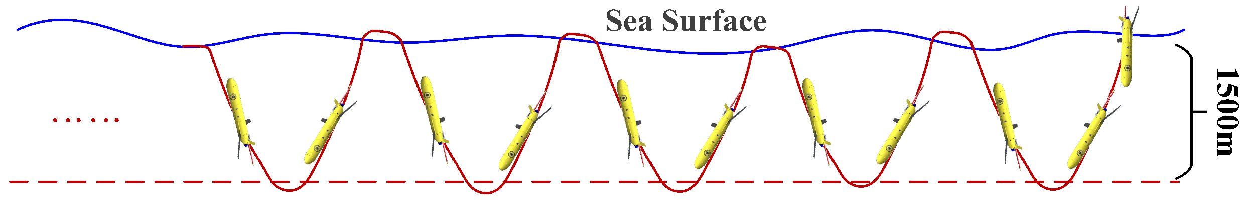
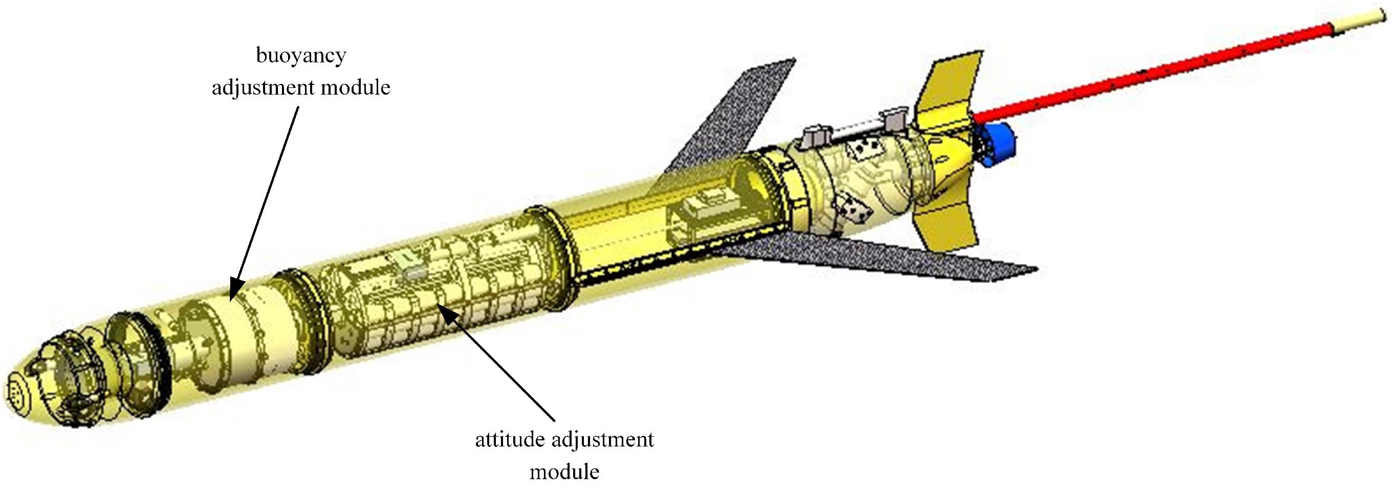
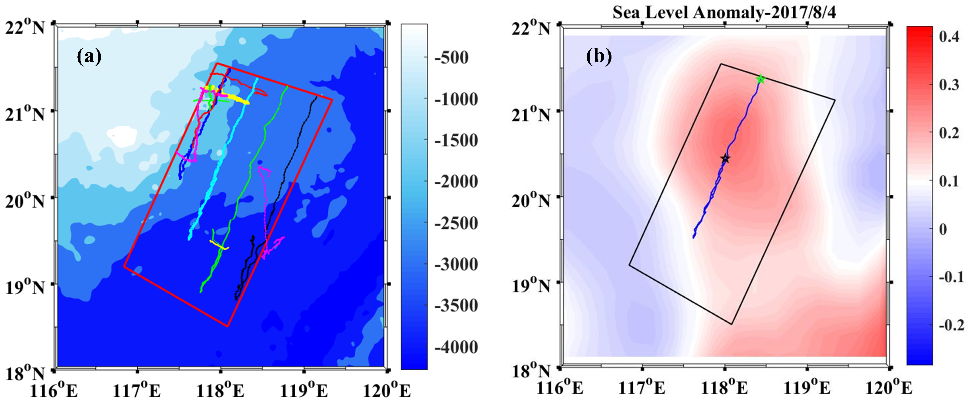
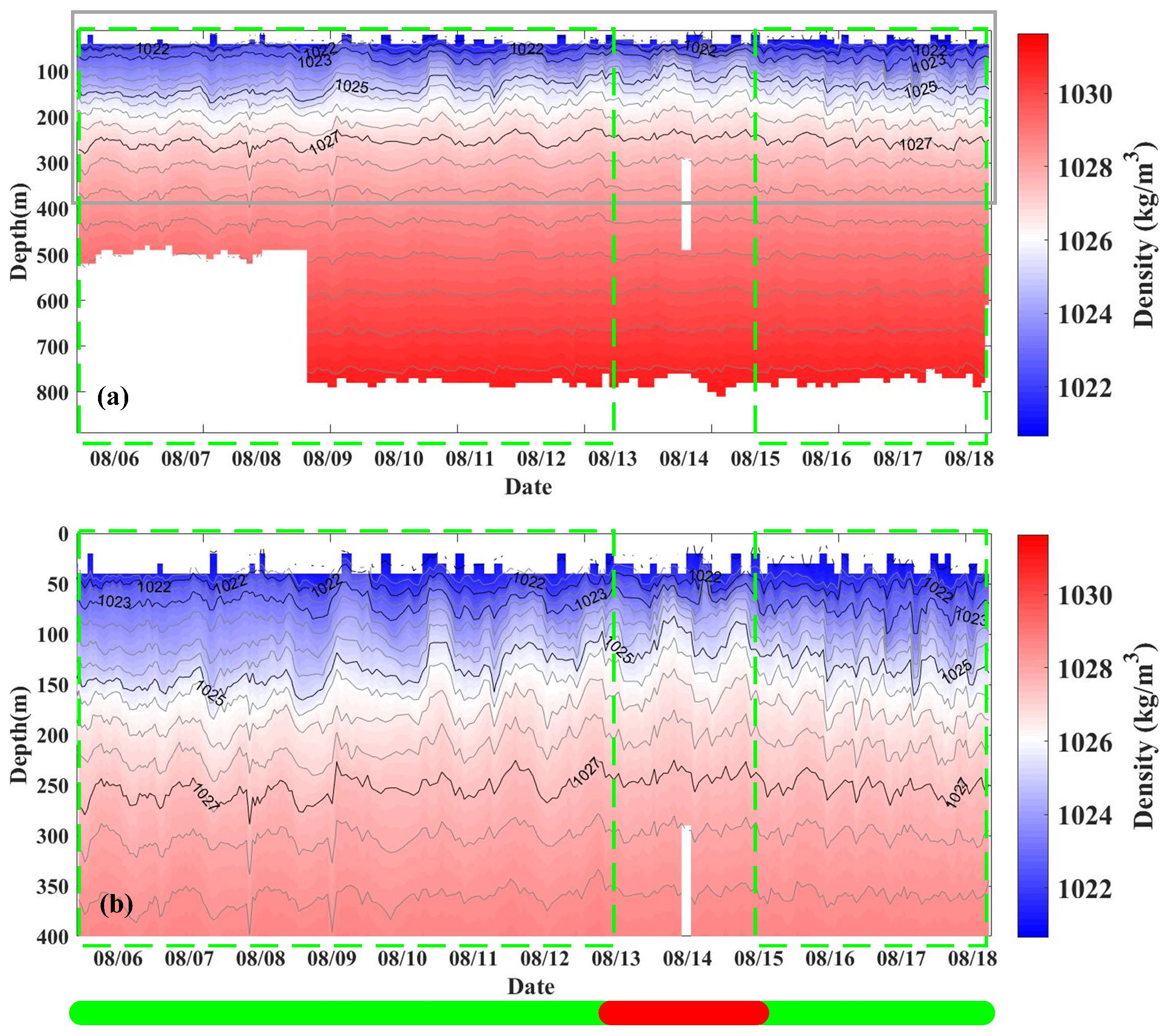
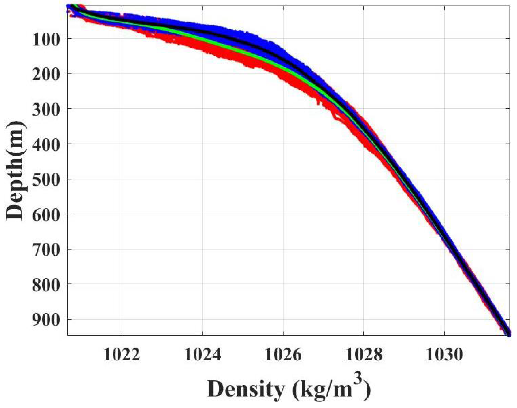
The South China Sea, as the largest and deepest marginal sea surrounded by the Asian continent and the islands of Kalimantan, Palawan, Luzon, and Taiwan in the western North Pacific Ocean, has a very complex submarine topography. The Asian monsoon system and its interactions with the coastline and submarine topography result in rich mesoscale eddies in the South China Sea. However, our understanding of the UGs motion performance inside mesoscale eddies remains incomplete. To reveal the motion characteristics of UGs within eddies, thus verify the effectiveness of their application in observing mesoscale eddies, and guide the design of a sampling scheme for mesoscale eddies observation, it is necessary to establish the dynamic model of the UG and simulate its motion process within an eddy. From 4 August 2017 to 29 August 2017, twelve “Petrel II” UGs developed by Tianjin University, China, were deployed in the northern part of the South China Sea, acquiring 1720 profiles totally. In this paper, the CTD (Conductivity-Temperature-with-Depth profiler) dataset collected by UGs and satellite data of SLA (Sea Level Anomaly) distributed by CMEMS (Copernicus Marine Environment Monitoring Service) are integrated. On this basis, we investigated the density distribution within the anticyclonic eddy, developed the dynamic model of “Petrel II” UG considering the buoyancy variation affected by both the density distribution within the eddy and deformation of the pressure hull, and conducted the analysis of the UG motion performance inside the eddy.
This paper is organized as follows:
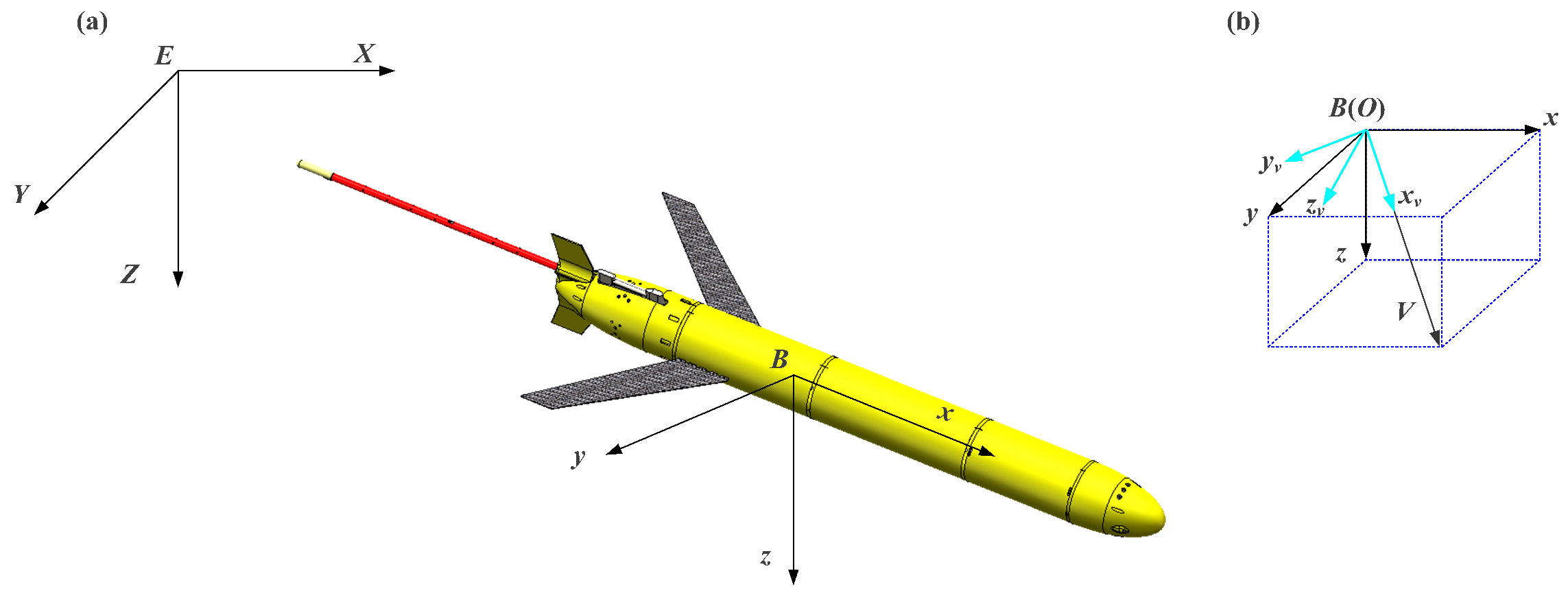
Section 2 describes the dynamic modeling of “Petrel II” UG, including kinematical modeling and force analysis, during which the density distribution within the eddy and deformation of the UG hull expressed as functions of ocean depth are introduced into the buoyancy analysis.
Section 3 investigates the dynamic behavior of “Petrel II” UG inside the anticyclonic eddy based on the constructed dynamic model.
Section 4 summarizes the full paper.
3. Results and Discussion
By considering the variations of the buoyancy, the validity and accuracy of the dynamic model in the vertical plane have been examined in
Section 2. In our research, the effect of the density distribution within the anticyclonic eddy on the dynamic behavior of “Petrel II” UG in the vertical plane is discussed thoroughly by analyzing the simulation results of the dynamic model established in
Section 2 with the density distribution inside (Model-1) or outside the eddy (Model-2). Same as the simulation setup of
Section 2.4, the net buoyancy (calculated by
), horizontal velocity, vertical velocity, gliding trajectory and pitch angle of the UG are obtained, as shown in
Figure 13,
Figure 14,
Figure 15 and
Figure 16.
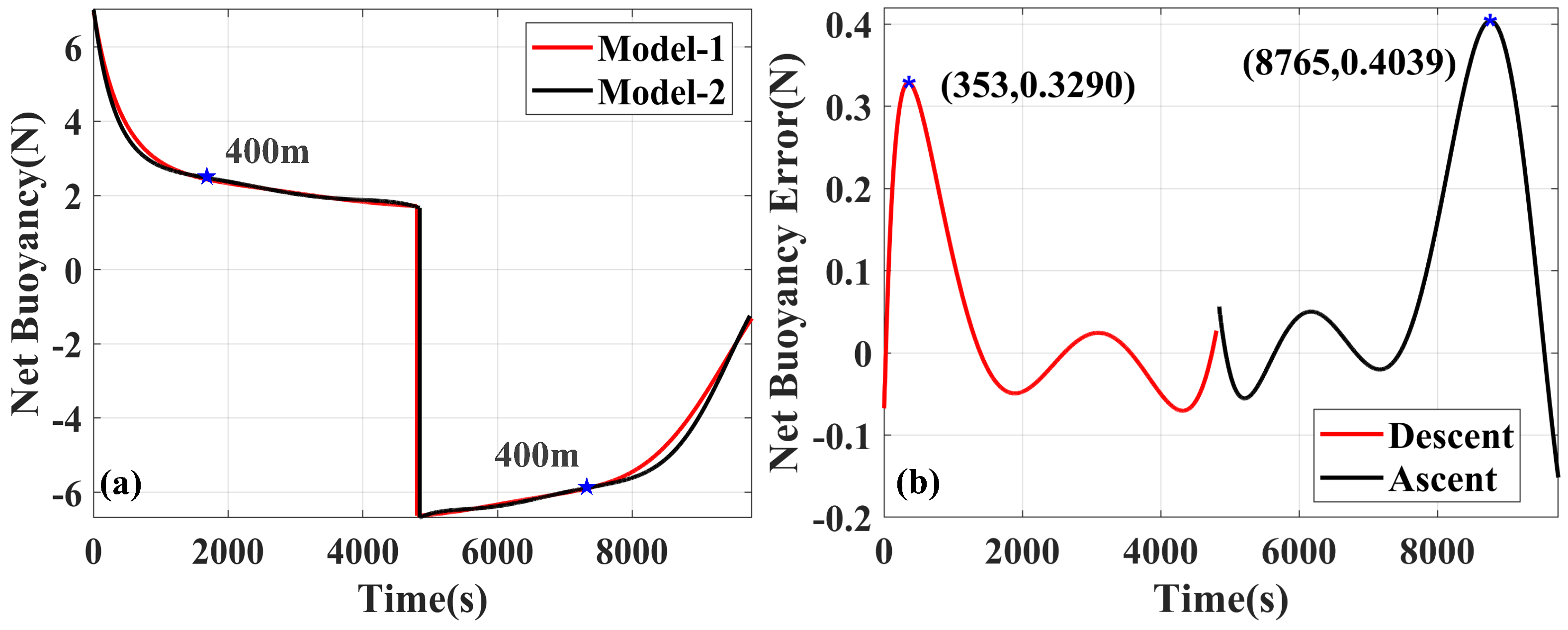
When the movement amount of the attitude adjustment module remains constant, the pitch angle increases with the increasing net buoyancy. It can be seen from
Figure 13a that there exists a slight difference in the net buoyancy of Model-1 and Model-2 during the diving (the value less than zero) and climbing (the value greater than zero) stages. The relevant data are listed in
Table 3. The net buoyancy decreases from 6.9467 to 1.7168 N during the descent and from 6.6337 to 1.3113 N during the ascent in Model-1, while in Model-2, it changes from 7.0142 to 1.6671 N and from 6.6844 to 1.2418 N in the descent and ascent, respectively. Obviously, there is a difference of about 0.3 N between the beginning of the descent and ascent both in Model-1 and Model-2, resulting from the compression deformation of the hull and variations of the seawater density. The same phenomenon also occurs at the end of the descending and ascending phases, with a difference of about 0.4 N. In Model-1, the net buoyancy varies dramatically between the sea surface and the depth of about 400 m with an average gradient of about 0.0027 N/m and 0.0019 N/m during the descent and ascent, respectively, while it changes slowly between 400 and 940 m with an average gradient of about 0.0002 N/m and 0.0003 N/m during the descent and ascent, respectively. The errors of the net buoyancy between Model-1 and Model-2 are calculated by subtracting the value of Model-2 from that of Model-1, as shown in
Figure 13b. In the descent, the error is within the range of −0.0703 N∼0.3290 N, and the maximum value of the errors reaches up to 0.3290 N at 353 s (about 107 m). Similarly, in the ascent, the value range of the error is [−0.1515 N, 0.4039 N] and the maximum value of the absolute errors achieves 0.4039 N at 8765 s (about 129 m). The results indicate that the larger error of the net buoyancy caused by the eddy density mainly occurs near the depth of the thermocline. Moreover, the estimated mean and standard deviation (
) of the absolute net buoyancy error are 0.0746 N and 0.0916 N, respectively, in the descent. However, they are 0.1150 N and 0.1317 N, respectively, in the ascent, which reveals a stronger influence of eddy density on the net buoyancy of the UG in the ascent than that in the descent.
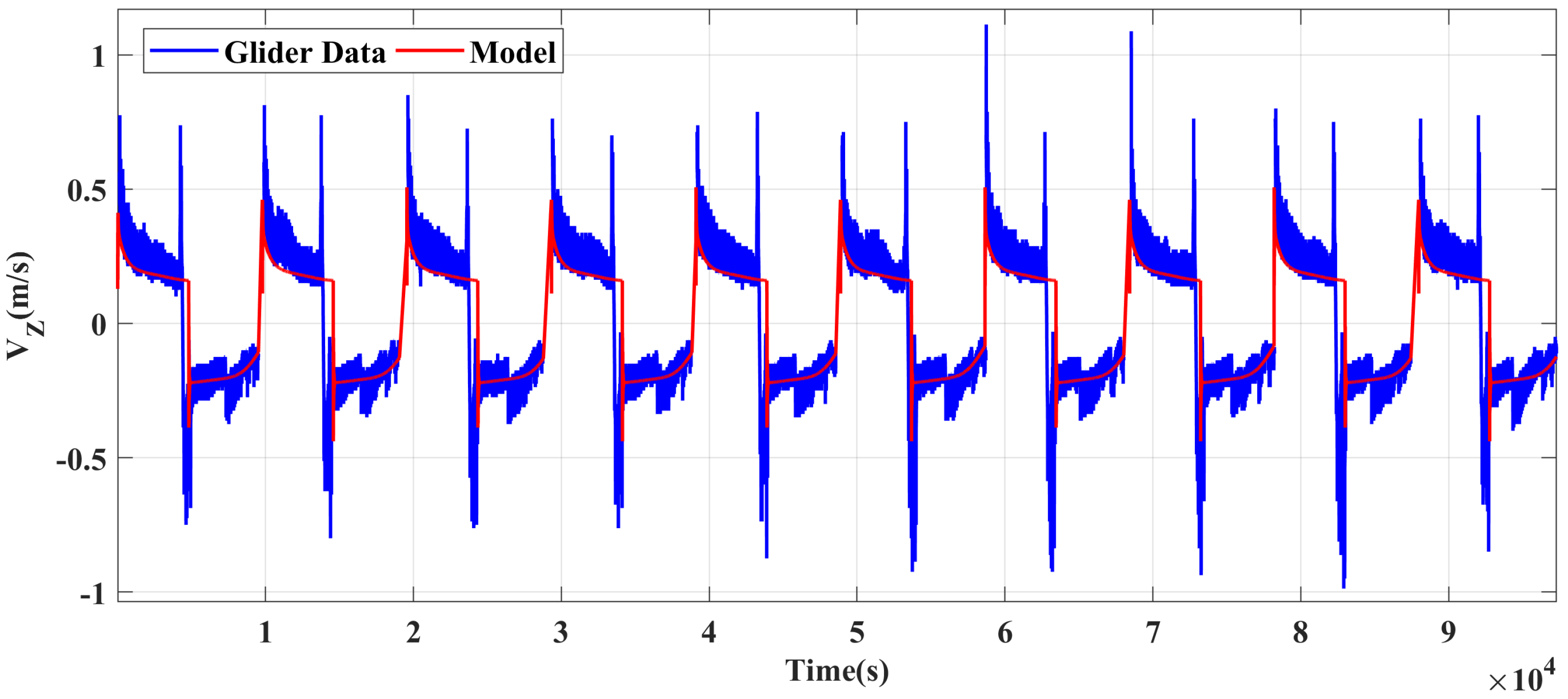
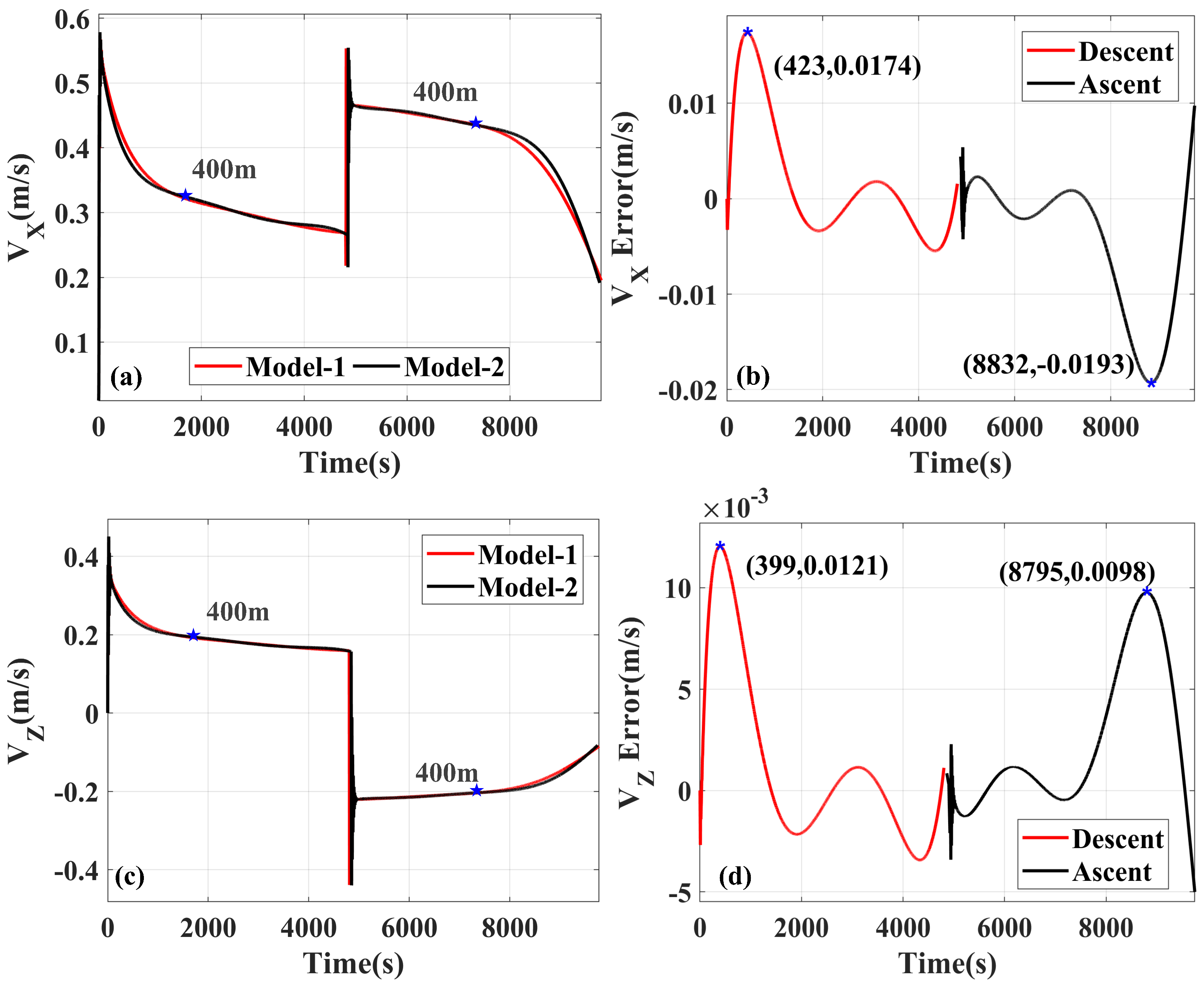
The simulation results of the horizontal (
) and vertical velocity (
) of the UG in the vertical plane are shown in
Figure 14a,c and
Table 4 and
Table 5. In Model-1,
and
in the descent decrease from 0.5292 m/s to 0.2686 m/s and from 0.3312 m/s to 0.1591 m/s, respectively. When switching from the decent to the ascent, both
and
change suddenly and fluctuate sharply due to the switch of input parameters, and they decrease from 0.4666 m/s to 0.2013 m/s and from 0.2204 m/s to 0.0876 m/s, respectively, when the UG moves steadily. Both
and
vary rapidly from the sea surface to 400 m depth but slowly from 400 to 940 m depth. In the climbing stage,
is larger at 400∼940 m depth with the mean value of 0.2133 m/s than that at a depth of 0∼400 m with the mean value of 0.1648 m/s, while in the diving stage, the variation of
is exactly opposite with
between 400 and 940 m smaller than that between 0 and 400 m. Then, at the same sampling frequency, the vertical sampling resolution of shallow water with a depth less than 400 m is higher than that of deeper water during the climbing of an UG. In the previous work, the vertical structures of temperature, salinity, density, chlorophyll, DO (Dissolved Oxygen) and CDOM (Colored Dissolved Organic Matter) within mesoscale eddies were discussed in detail [
4], which revealed that the anomalies within eddies were mainly distributed in the depth of 0∼400 m. To obtain more details of the eddy structure, the climbing profiles are chosen as the available profiles to capture the eddies. Suppose the data are collected in the descent. In that case, it is necessary to increase the sampling frequency of the sensors between the sea surface and 400 m and reduce that from 400 to 940 m to obtain a reasonable vertical sampling resolution. In Model-2, the variation trends of
and
are similar to those in Model-1.
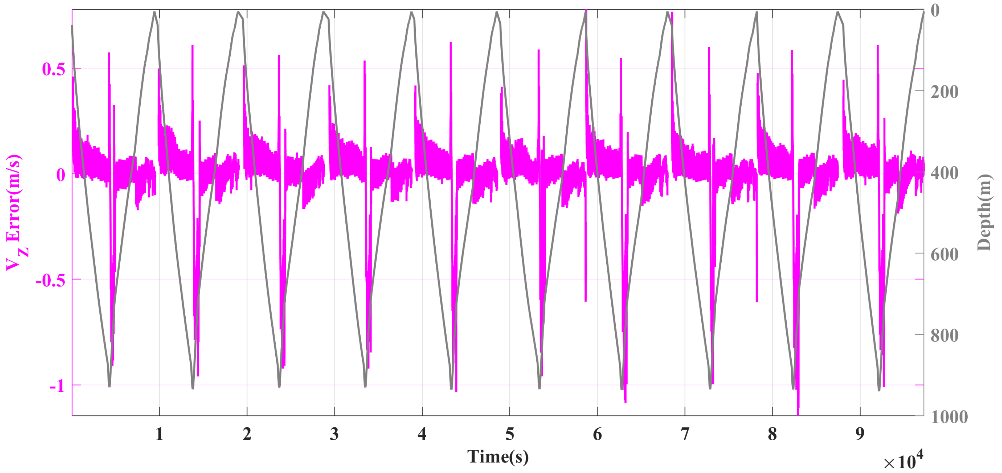
To illustrate the differences between the two models in more detail, the errors of
and
are represented in
Figure 14b,d, respectively. Both positive and negative values of
error show a large fluctuation, as seen in
Figure 14b. The outliers found between the descent and ascent are caused by switching input parameters and considered as the invalid data. It can be observed that the curve of the
error has an approximately centrosymmetric structure and the errors fall in the range of −0.0055 m/s∼0.0174 m/s with the maximum of 0.0174 m/s at 423 s (about 126 m) in the descent and a wider range of −0.0193 m/s∼0.0097 m/s with a larger maximal error of 0.0193 m/s at 8832 s (about 128 m) in the ascent. So, the larger errors appear near 120 m, whether in the descent or the ascent, meaning the greater impact of the eddy density on the horizontal velocity at a depth of about 120 m. For the absolute value of
error, the mean and
values are 0.0045 m/s and 0.0049m/s, respectively, in the descent. However, in the ascent, the mean is 0.0055 m/s, and the standard deviation of 0.0064 m/s, which are both larger than those in the descent. Thus, there is a stronger influence of the eddy density on
in the ascent than that in the descent. Different from the variation of
error, the error of
shows an approximately axisymmetric structure. In the descent, the fluctuation with the range of −0.0034 m/s∼0.0121 m/s is slightly greater in magnitude than that in the ascent with the range of −0.0050 m/s∼0.0098 m/s. At 399 s (about 120 m) in the descent and 8795 s (about 124 m) in the ascent, there exist two larger peaks of
error, indicating that the eddy density has more influence on the vertical velocity at a depth of about 120 m. To estimate the mean and
, the absolute values of
error are calculated. The mean and
values are 0.0030 m/s and 0.0034 m/s in the descent, respectively. In the ascent, they are 0.0029 m/s and 0.0036 m/s, respectively. So, there is little difference in the influence of the eddy density on
in the descent and ascent.
To reveal how the eddy density affects the movement position of the UG, the simulation results of its gliding trajectory and pitch angle are displayed in
Figure 15 and
Figure 16 and
Table 6. In
Figure 15a, the two trajectories obtained from the simulation using Model-1 and Model-2 almost overlap. However, the time required for an UG to complete a profile simulated based on Model-1 is slightly longer than that based on Model-2, which indicates that the difference of the out-of-water moments simulated by the two models will keep increasing as the number of UG gliding profiles increases. Compared with the simulation results of Model-2, it takes less time for an UG to dive to the specified depth in Model-1 but more time to climb to the sea surface. In order to discuss the trajectory error in more detail, the error between the trajectories simulated by the two models is calculated, as shown in
Figure 15b. It can be found that the error fluctuates in both the descent and ascent. In the descent, the error increases gradually from zero to the maximum absolute value of 9.5588 m at 1402 s, when the trajectory obtained from Model-1 reaches 342.6826 m and that obtained from Model-2 achieves 333.1238 m. Then, the error locates at the larger values and fluctuates with a small amplitude, which is consistent with the phenomenon in
Figure 14d, where the error of
fluctuates around the value of zero in this stage. In the ascent, the trajectory error reaches the maximum absolute value of 9.1305 m at 5649 s, when the trajectory obtained from Model-1 reaches 755.0830 m, and that obtained from Model-2 reaches 764.2135 m. During the stage of the simulation time larger than 5649 s, the trajectory error also fluctuates near the larger values with a small amplitude and then gradually decreases to zero. Hereafter, it starts to grow in a positive direction because of the
error still being greater than zero. When the error of
is less than zero, the trajectory error starts to decrease. To compare the effect of the eddy density on the trajectory errors in the descent and ascent, the variations of the absolute trajectory error in the two phases are discussed. In the descent, the mean value of the absolute trajectory error is 7.4059 m with the Std value of 2.2284 m, while in the ascent, the mean and
values are 6.7365 m and 2.7849 m, respectively. Obviously, the mean value in the descent is larger than that in the ascent, but the
value is smaller. So, the coefficient of variation (
,
) is adopted as a normalized index to measure the error dispersion. The
is calculated to be 0.3009 for the descent and 0.4134 for the ascent, indicating that the trajectory error in the ascent has the larger variability and the trajectory is more influenced by the eddy density, which is consistent with the conclusions discussed above.
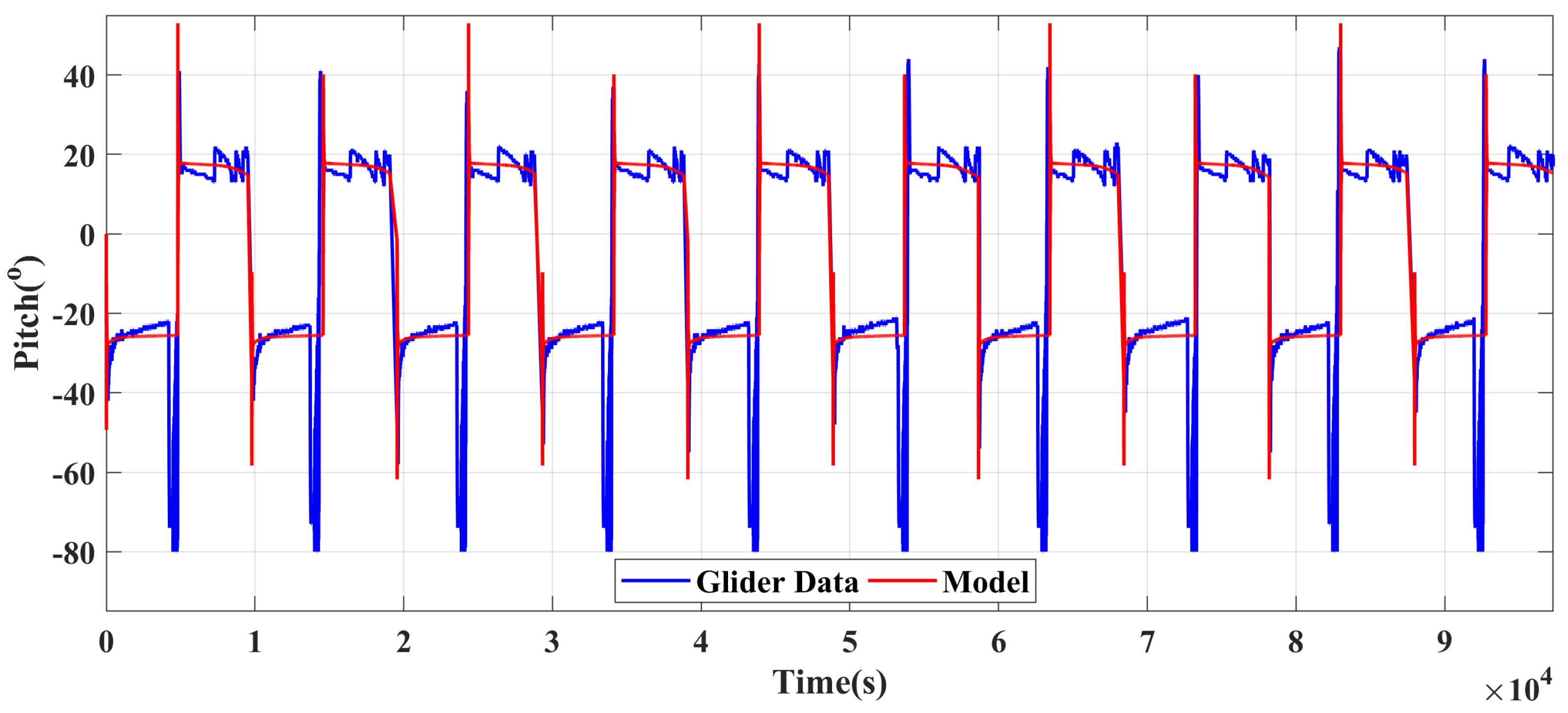
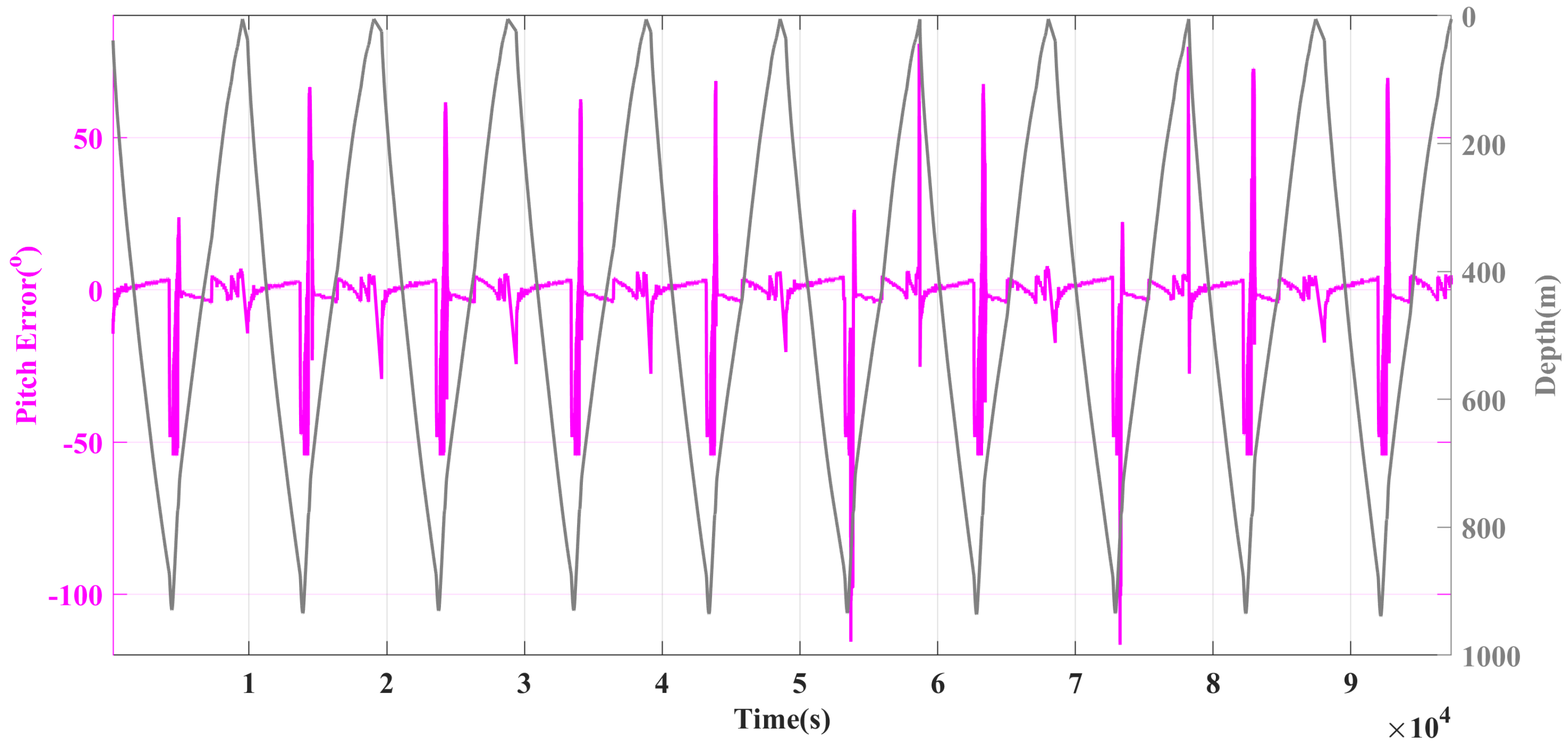
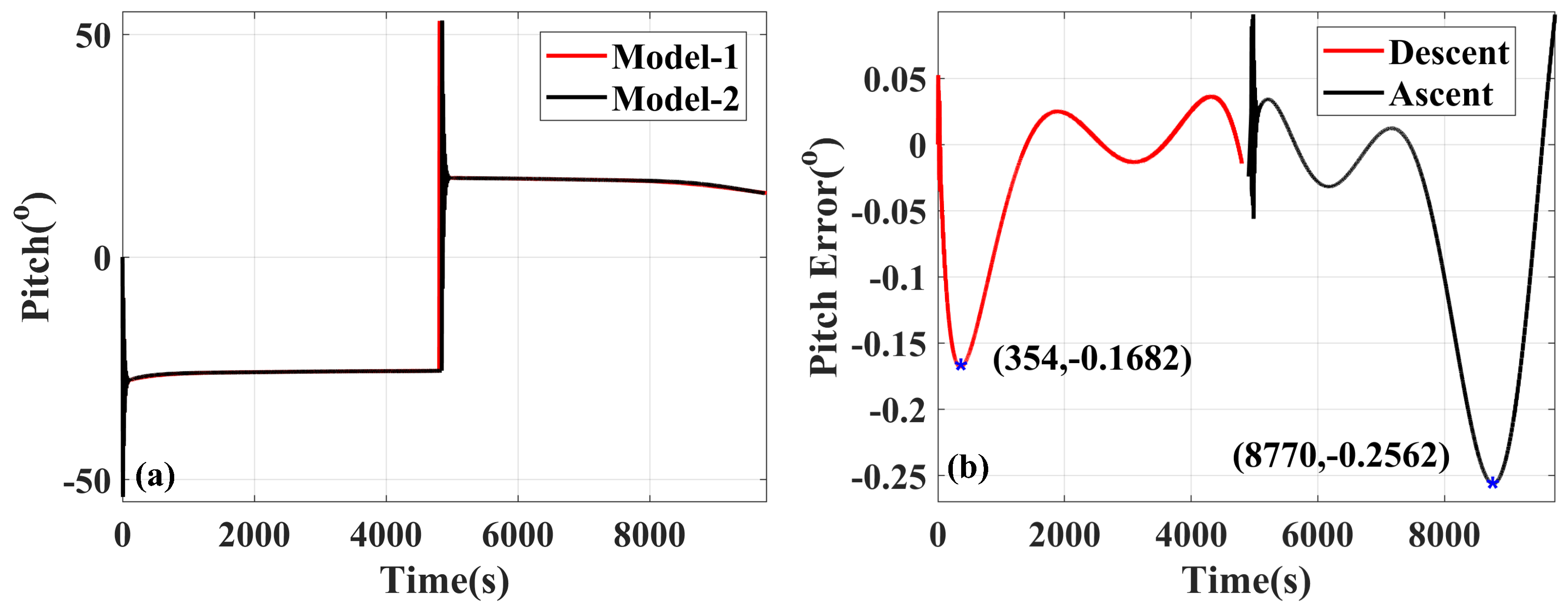
As shown in
Figure 16a and
Table 7, the pitch angle of the UG simulated in Model-1 decreases gradually from 27.4562° to 25.5568° in the descent and from 17.7683° to 14.3615° in the ascent. Similar to the variation in Model-1, the pitch angle obtained from Model-2 also decreases from 27.3256° to 25.5320° in the descent and from 17.7879° to 14.3175° in the ascent. To illustrate the difference in the pitch angle between the two models, the simulation results of the pitch angle error in the vertical plane are shown in
Figure 16b. In the descent, the maximum absolute error of 0.1682° occurs at 354 s (about 108 m). Then, the error values fluctuate in a small range. In the ascent, the maximum absolute error of 0.2562° appears at 8770 s (about 128 m). According to the above analysis of the gliding trajectory, the UG simulated in Model-1 reaches the specified depth before Model-2, meaning that the pitch angle in Model-2 keeps the positive value when that in Model-1 switches to the negative value. Therefore, there exists a difference of about 20 m between the depth of the maximum error in the descent and ascent. The mean and Std values of the absolute pitch angle error are 0.0384° and 0.0469°, respectively, in the descent, while these values are 0.0746° and 0.0840°, respectively, in the ascent, both of which are greater than those in the descent, indicating that the mesoscale eddy density makes a stronger effect on the pitch angle of the UG in the ascent.
4. Conclusions
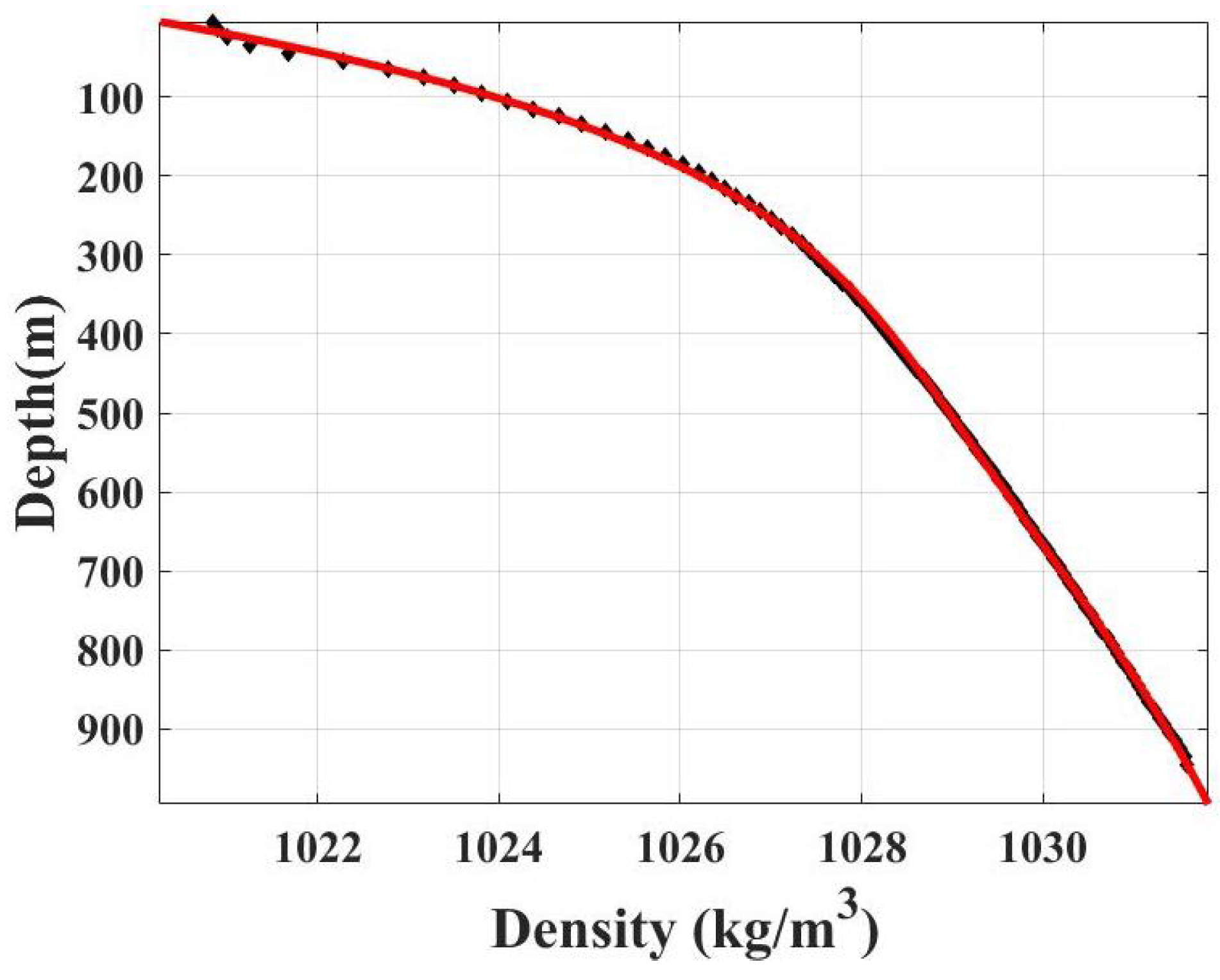
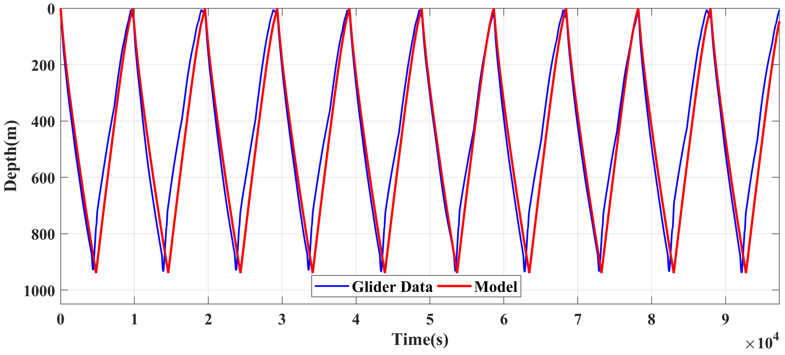
Considering the effect of the density distribution within an eddy on the buoyancy of “Petrel II” UG, the distribution of the eddy density is fitted by a quintic polynomial based on the data collected by a “Petrel II” UG in the sea trial. By combining with the compressibility of the pressure hull, we derive the new expressions of the UG buoyancy which are rewritten as the functions of the water depth h, and thus, the new dynamic model of the UG is established. Assuming there is negligible effect of the vertical velocity inside the anticyclonic eddy on the motion of UG, the analysis of the in situ UG data proves that the established dynamic model has high accuracy in predicting the motion performance of UGs within an eddy in the vertical plane, demonstrating the validity and availability of the dynamic model considering the effect of the density distribution within the eddy to analyze the dynamic behavior of UGs inside an eddy. Based on the established dynamic model, the motion performance of the UG considering the density distribution within the eddy is analyzed.
There is a slight difference in the magnitude of the net buoyance when the dynamic model integrates the density distribution inside an anticyclonic eddy (Model-1) or not (Model-2). In Model-1, there exists a dramatic variation exists from the sea surface to about 400 m depth but a slow variation from about 400 to 940 m depth. The maximum values of the absolute errors between Model-1 and Model-2 reach up to 0.3290 N and 0.4039 N during the descent and ascent, respectively. When the error reaches its maximum values, the depths arrived by the UG simulated with Model-1 are 107 m and 129 m in the descent and ascent, respectively, meaning that the larger error of the net buoyancy caused by the eddy density mainly occurs near the depth of the thermocline. The estimated mean and standard deviation of the absolute net buoyancy are 0.0746 N and 0.0916 N in the descent, respectively, and 0.1150 N and 0.1317 N in the ascent, respectively, indicating that there is a stronger influence of eddy density on the net buoyancy of the UG in the ascent than that in the descent. In Model-1, the value of the horizontal velocity and the vertical velocity in the descent decreases from 0.5292 m/s to 0.2686 m/s and from 0.3312 m/s to 0.1591 m/s, respectively, while in the ascent, they decrease from 0.4666 m/s to 0.2013 m/s and from 0.2204 m/s to 0.0876 m/s, respectively. Similar to the variation of the net buoyancy, both the horizontal velocity and vertical velocity vary rapidly from the sea surface to 400 m depth but slowly from 400 m to 940 m depth. In the ascent, the vertical velocity value is larger at 400∼940 m depth than that at a depth of 0∼400 m. Considering the vertical velocity variations of the UG and the vertical structures of parameters within eddies, the climbing profiles are chosen as the available samples to capture an eddy. If the diving profiles are chosen, increasing the sampling frequency of sensors between the sea surface and 400 m and reducing that from 400 to 940 m will facilitate a reasonable vertical sampling resolution. The curve of the error shows an approximately centrosymmetric structure, and the maximum of the errors is 0.0174 m/s located at about 126 m in the descent and 0.0193 m/s located at about 128 m in the ascent, which means that the larger errors appear near 120 m whether in the descent or the ascent, revealing the greater impact of the eddy density on the horizontal velocity at a depth of about 120 m. In the descent, the mean and standard deviation values of the absolute error are 0.0045 m/s and 0.0049 m/s, respectively. In the ascent, they are 0.0055 m/s and 0.0064 m/s, respectively, which are both larger than those in the descent, showing a stronger influence of the eddy density on in the ascent than that in the descent. When discussing error, it can be found that there exist two larger peaks of error at about 120 m in the descent and about 124 m in the ascent, indicating that the eddy density has more influence on the vertical velocity at a depth of about 120 m. Moreover, the mean and standard deviation values are 0.0030 m/s and 0.0034 m/s in the descent, respectively. In the ascent, they are 0.0029 m/s and 0.0036 m/s, respectively, which gives us an important conclusion that there is little difference in the influence of the eddy density on in the descent and ascent. Moreover, the time required for an UG to complete a profile simulated by Model-1 is slightly longer than that by Model-2. Comparing the simulation results of Model-1 with those of Model-2, it takes less time for an UG to dive to the specified depth in Model-1 but more time to climb to the sea surface. The maximum values of the depth error are located at 9.5588 m and 9.1305 m in the descent and ascent, respectively. The coefficient of variation is calculated to be 0.3009 for the descent and 0.4134 for the ascent, indicating that the trajectory error in the ascent has a larger variability and the eddy density more influences the trajectory. The pitch angle of the UG simulated both in Model-1 and Model-2 decreases gradually both in the descent and ascent. The simulation results of the pitch angle error in the vertical plane show that the maximum error of 0.1682° occurs at about 108 m in the descent and 0.2562° appears at about 128 m in the ascent. In the descent, the mean and standard deviation values of the absolute pitch angle error are 0.0384° and 0.0469°, respectively, while these values are 0.0746° and 0.0840° in the ascent, respectively, both of which are greater than those in the descent, indicating that the mesoscale eddy density makes a stronger effect on the pitch angle in the ascent.
The dynamic model of “Petrel II” UG considering the effect of the density distribution within the eddy contributes to the research on the motion performance analysis of the UG in the complex density distribution within an eddy, which demonstrates that the established dynamic model can predict the movement of the UG in the environment with the complex density distributions. The detailed analysis of the simulation for the dynamic model integrating the density distribution inside an anticyclonic eddy or not shows the differences in the effect of the mesoscale eddy density on the motion performance of “Petrel II” UG in the descent and ascent. Moreover, the results provide a sampling suggestion for applying UGs in the mesoscale eddy observation.


