Collaborative Optimization of Yard Crane Deployment and Inbound Truck Arrivals with Vessel-Dependent Time Windows

Abstract

Due to mega-ships, increasing container throughput, and nonuniform truck arrivals, many container terminals face challenges of unbalanced workloads of yard equipment, shortage of equipment resources in peak hours, and congestion problem. To solve such issues, we propose a mixed-integer bilevel programming model to optimize the vessel-dependent time windows for inbound trucks and yard crane deployment simultaneously. In the proposed bilevel model, the upper level aims to minimize the total truck waiting time at the container terminal gate and yard, while the lower level is formulated to minimize the total workload overflow to next shift in the whole container yard. The optimal yard crane deployment obtained in the lower level will transfer to the upper level problem to determine the waiting time of trucks in the yard and then affect the truck arrivals pattern. To solve the model, a hybrid algorithm—called hybrid genetic algorithm, based on collective decision optimization—is put forward by combining the genetic algorithm and the collective decision optimization algorithm. Numerical experiments are conducted to validate the proposed approach is effective to simultaneously flatten truck arrivals and improve the efficiency of yard cranes. The proposed approach can significantly reduce container terminals’ truck waiting time.

1. Introduction

Maritime transport, as an economic and environmental-friendly transport mode, is playing an increasingly important role in international trade [1]. The emergence of containers has changed the method of freight transport through sea routes. Containerization has greatly improved port handling efficiency and lowered freight rates [2]. After the development of more than half a century, container liner shipping has become one of the most important transportation modes in international trade. Statista reported that approximately 60% of all world seaborne trade in terms of value is carried by container ships [3].

Nowadays, maritime container terminals have to face increasingly tough requirements by shipping companies which claim real-time services [4]. In order to be selected as hub ports or origin–destination points in shipping routes, marine container terminals have to improve their management capabilities and productivity [5,6,7,8]. Furthermore, liner shipping companies continue to increase the scale of deep-sea container vessels, as larger vessels can lower voyage costs per container due to economies of scale. The carrying capacity of container ships has increased significantly over the last 50 years [9]. Generally, the external trucks arrive at the marine container terminal randomly and nonuniformly within the time window assigned to the vessel by the container terminal. If the time window assignment is unreasonable, such as the overlapping of time windows, and the length of the time windows does not match with the volume of outbound containers, it will lead to a large number of trucks moving in and out of the terminal during peak hours. Truck arrivals exceeding the capacity of the gate and yard can lead to heavy congestion.

Therefore, how to increase the efficiency of pickup and delivery operations by trucks and avoid truck congestion is an important issue for terminal operators, truck fleets and government regulators. In recent years, marine container terminals have adopted some measures to alleviate congestion. According to the formula of utilization factor $\rho$, Motono et al. [10] divided these congestion alleviation measures into three categories. The first category is increasing the number of servers, such as gate lanes and yard cranes. The second category is controlling truck arrival rate by truck arrival management (TAM). The third category is improving gate service rate by managerial and technological methods. Quite a few studies have focused on the TAM, mainly including the truck appointment system (TAS), vessel-dependent time windows (VDTWs) and tariff/toll pricing policies (TTPP). These measures can be combined if necessary.

The TAS was first introduced in the Vancouver port of Canada, and many marine container terminals in North America followed. At present, the ports of Los Angeles and Long Beach in America [11] and Tianjin port in China have implemented TAS. By assigning appointment quotas to the maximum amount of trucks that can be accepted per period, the TAS can regulate off-peak truck deliveries and reduce trucks’ congestion at the container terminal. Furthermore, TAS could provide information about truck arrival time windows. Utilizing the incomplete truck arrival information can also improve the efficiency of yard operations in terms of reducing container rehandles [12,13,14]. Therefore, it is necessary to design the TAS scientifically. Huynh and Walton [15] simulated the operation process of trucks in container yards to obtain the average turn time of trucks, then a mathematical formulation was applied to determine the optimal number of trucks that could enter the yard per time window. In order to determine the optimal appointment quotas, the non-stationary queueing models were used to describe the queuing process of trucks at the gate and yard of the container terminal [16]. The essence of TAS is shifting truck arrivals from peak to off-peak periods. However, the arrival time adjustments will bring inconvenience to the truck drivers. To fix this problem, Chen et al. [17] developed a bi-objective optimization model that minimizes both truck waiting times and the number of shifted truck arrivals. Phan and Kim [18,19] proposed an improved concept in which truck companies and the terminal operator collaboratively determine truck operation schedules and truck arrival appointments. Container terminals can not only use TAS to relieve terminal congestion, but also use the appointment information obtained from TAS to optimize the storage space allocation problem in container yards [20].

Another method of TAM is the VDTW method, which can also manage off-peak inbound truck arrivals and reduce truck congestion significantly. Its original purpose was to utilize the truck arrival patterns of each vessel to optimize delivery time windows for outbound containers to minimize the total system cost [21,22]. Chen and Jiang [23] systematically discussed the practical application of three optimized alternative time window strategies, including fixed ending-point strategy, variable end-point strategy and greedy algorithm strategy. Ma et al. [24] established an optimization model to assign a time window for inbound trucks of each vessel and appointment quota for each appointment period to minimize the total carbon dioxide emissions of trucks and rubber tired gantry cranes (RTGCs) during idling. The truck arrival pattern within a time window is the backbone of the VDTW method. Some of these studies assumed that the arrivals of outbound containers within a time window follow the Beta distribution [21,22,23]. However, it is well known from theory and experience that there may be a substantial gap between an assumed theoretical parametric distribution and the physical behavior of historical data [25]. Beta distribution may work well for some container terminals, such as the container terminal of Tianjin Port, but may not work for others. To address the inadequacies associated with present parametric density estimations for containers’ delivery and pick up time distributions, Ma et al. [26] proposed a novel estimation method for distribution function estimation using a non-parametric estimation method called kernel distribution function estimators (KDFEs).

The TTPP motivates truck arrivals to shift from peak periods to off-peak periods by charging a higher traffic mitigation fee (or toll fee) for trucks entering the marine container terminal during peak hours. In recent years, it has been adopted by the Port of New York and New Jersey and the Ports of Los Angeles and Long Beach. Peak toll is successful to spread peak period traffic to the periods before or after it [27,28]. Chen et al. [2] combined the TAS with a time-varying pricing system that leads to the optimal arrival pattern. In order to determine the optimal toll rates, Zhang et al. [29] developed a bi-level programming model, considering the game relationship among container terminal operators, truckers and government regulators.

Trucks concentratedly arriving at the terminal to pick-up or deliver containers not only results in truck congestion, but also in the low utilization of container terminal equipment. Furthermore, the level of workload in different blocks is uneven and changes dynamically over time. As a result, container terminals rarely ever utilize the yard crane capacity to the fullest. Truck arrivals and yard crane scheduling rely on each other to achieve a good performance in pickup and delivery operations. Therefore, Zehendner et al. [30] proposed a mixed integer linear programming model for the optimization of appointment quotas and the allocation of straddle carriers to different transport modes. The model improved not only the service quality of trucks, but also of trains, barges and vessels. However, for the container yard served by gantry cranes, the gantry crane cannot move from one block to another in the same period as frequently as the straddle carrier. In order to get the well-designed yard crane deployment, it is necessary to obtain the workload of each block in each period. Therefore, it would be better to specify in which block the container is going to be when making the appointment. Ma et al. [31] developed a bi-level programming model for the optimization of appointment quotas of each block in each period and RTGC deployment. In order to balance the interests of container terminals and truckers, Li et al. [32] set up a bi-objective integer model to optimize appointment quotas and yard cranes deployment in container deliveries simultaneously.

Most of these previous researches have focused on various strategies of truck arrival management for reducing congestion. Some studies shorten the waiting time of trucks in the yard and reduce the number of yard cranes deployment through the joint optimization of appointment quotas and yard cranes deployment, However, appointment quota optimization ignores the fact that the traffic flows of trucks for container pickup and delivery are triggered by vessel arrival. The processes of assigning time windows for inbound trucks of each vessel and RTGC deployment were not carried out at the same time in previous studies. The VDTWs method is an effective measure of truck arrival management. It can not only reflect that the traffic flow of trucks is triggered by vessel arrival, but also consider the arrival pattern of inbound trucks within the delivery operation time window. Therefore, the VDTWs arrangement for inbound trucks and RTGC deployment was modeled using mixed-integer bilevel programming. This research contributes to the literature by (1) developing a mixed-integer bilevel programming model, which can optimize the VDTWs and RTGCs deployment simultaneously; (2) considering the destination yard blocks information of outbound containers and the storage capacity constraint of yard blocks; (3) proposing a new approach, namely kernel distribution function estimators (KDFE), to estimate the distribution pattern of truck arrivals within the time window. Thus, the container terminal operators can assign the time windows for outbound containers reasonably and assign yard cranes to correct blocks at proper time moments, so as to ensure the matching of workload and service capacity, and significantly reduce truck waiting time.

The remainder of this paper is organized as follows. Problem description and optimization model for time windows arrangement and RTGC deployment are given in Section 2. A synchronous scheduling optimization algorithm for yard cranes deployment and VDTWs arrangement is designed in Section 3. Section 4 tests the model performance with a case study of a Chinese maritime container terminal. Conclusions are provided in Section 5.

2. Problem Formulation

2.1. Problem Description and Assumptions

In the outbound container delivery process, the container terminal operator would assign a specific time window for each vessel after receiving the arrival announcement and informs all the related shippers or distribution centers. Then, the shippers sent container delivery orders to trucking companies. The trucking companies designate trucks to transport outbound containers to the container terminal within the time window according to their capacity. As shown in Figure 1, when the truck delivering outbound containers arrives at the terminal gate, it usually needs to join a queue due to documentation, container inspection and congestion inside the container yard. After passing through the terminal gate, the truck proceeds to the specific block, where the container will be stored within the container yard, according to the indication given by the terminal gate. When the truck arrives at that block, it also needs to join a queue waiting for the yard cranes, working at that block, to remove the container from it. After the yard crane puts the outbound container in the correct storage position, the truck will either leave the terminal directly or retrieve an import container.

From the trucker’s point of view, the shorter the waiting time at the container terminal, the better. However, reducing the waiting time by increasing the number of servers (that is, yard cranes deployed to each block) means that the operating cost of the terminal will increase. A well-designed yard crane deployment is essential to achieve maximum efficiency. Therefore, the terminal operator can further decrease trucks’ waiting time by making yard crane deployment match truck arrivals. However, in some practical situations, an idle yard crane is randomly pulled out of a block and moved to another congested block according to the artificial experience. In this paper, VDTW assignment and RTGC deployment are modeled using bilevel programming.

The flowchart of VDTW assignment and RTGC deployment is shown in Figure 2. After the vessel departs, the yard space occupied by outbound containers corresponding to the vessel can be released. It means that the vessel ETD (estimated time of departure), outbound container volume of each vessel and storage capacity of each block directly determine the available storage capacity of each block. However, the starting point of VDTW depends on the available storage capacity of the block where the corresponding outbound containers can be stored [23]. In addition, the ending point of VDTW depends on vessel cut-off time. Therefore, firstly, we assign a specific time window for each vessel according to vessel cut-off time, vessel ETD, outbound container volume of each vessel and the storage capacity of each block. Then, we use the kernel distribution function estimators developed by Nadaraya [33] to estimate truck arrivals of each vessel during each period based on the given set of time windows. Next, we make the optimum RTGC deployment that minimizes the work overflow to the next period of all blocks. According to the RTGC deployment, the number of RTGCs available at each block can be obtained in real time. Afterward, the average number of trucks waiting at the gate lanes and blocks is calculated using the time-dependent queue model. If the congestion is acceptable, the terminal operator will adopt the time windows and informs all the related shippers or distribution centers. Otherwise, the time windows should be modified. Furthermore, the RTGC deployment should be optimized again, and the average number of trucks waiting at the gate lanes and blocks should also be recalculated.

2.2. Vessel Dependent Time Windows

The container terminal allocates a time window to each vessel by assigning the open time and cutoff time of the container yard to each vessel’s outbound containers. Furthermore, the distribution of inbound truck arrivals during the time window obeys some laws. The cumulative distribution function of outbound container arrival rate during the time window can be obtained by the probability distribution fitting method based on the historical data of vessels’ time windows in the past voyage and the arrival time of outbound containers. After obtaining the arrival time distribution of outbound containers in the time window, truck arrivals can be controlled by rationally assigning the time window. This truck arrival management method is named ‘vessel-dependent time windows’ (VDTWs) [21,22].

When excavating the arrival time distribution of outbound containers in the time window, some studies assume that the arrival probability of the outbound containers in the time window follows Beta distribution [21,22,23]. Then, the unknown parameters of the assumed distribution model are estimated and tested. However, in reality, not all the cumulative distribution of container arrival time at container terminal is consistent with the known classical distributions, such as normal distribution, beta distribution and uniform distribution. The kernel distribution function estimators (KDFEs) can only rely on historical data to infer the distribution without assuming that the distribution follows a certain pattern. It just makes up for the shortage of the parameter estimation method in fitting the distribution of outbound container arrival time. Therefore, this paper uses the KDFE method to estimate the cumulative distribution function of the outbound container arrival time. See Appendix A for the specific steps of the KDFE method.

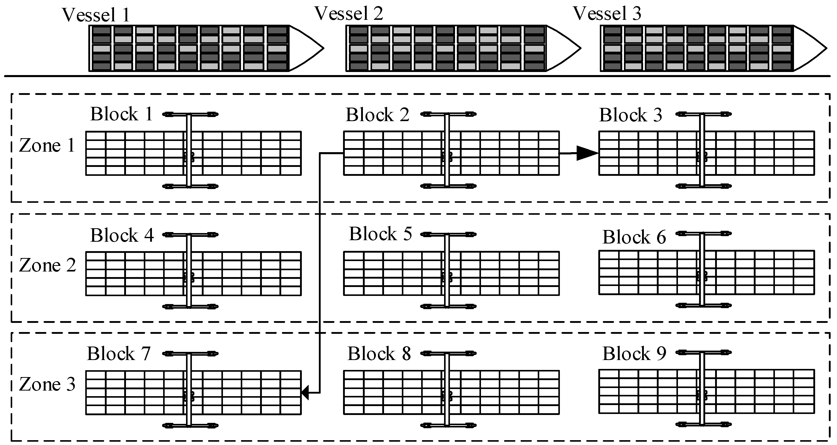
2.3. Container Yard Operation and RTGC Deployment

The container yard in a container terminal is divided into several blocks. The terminal operation system will indicate those inbound trucks entering the gate to transport the outbound containers to the designated blocks for storage according to the yard plan. According to the stowage plan supplied by liner shipping company and the storage position of the outbound containers in the yard, the container terminal makes the operation stowage plan. After the vessel is berthed, the container terminal will command the internal trucks and quay cranes to complete the vessel loading and unloading, cooperatively, according to the operation stowing plan [34]. The most commonly used yard cranes in the container yard are RTGC and rail mounted gantry cranes (RMGCs). Because the outbound containers of different vessels are stored in different blocks, the distribution of the outbound containers and inbound trucks flow in the container yard is unbalanced in time and space. In order to make full use of the operational capacity, the yard cranes need to be transferred to the blocks with more tasks after completing a small number of tasks in the idle blocks. Therefore, compared with RMGCs, which are fixed to a block, RTGC deployment is more meaningful for improving yard operation efficiency. As shown in Figure 3, a row of blocks, parallel to the shoreline, constitutes a Zone (e.g., blocks 1, 2, and 3 belong to Zone1, blocks 4, 5, and 6 belong to Zone2). The RTGC can move freely between two adjacent blocks in the same Zone. If a RTGC wants to move from a block in one Zone to a block in another Zone (e.g., move from block 2 to block 7), the RTGC needs to make two 90° turns. In addition, RTGCs cannot cross each other generally, so one RTGC cannot cross other blocks when transferring from one block to another. For example, the RTGC shown in Figure 3 cannot directly transfer from block 1 to block 3, 6 or 9.

2.4. Assumptions and Notations

2.4.1. Assumptions

The assumptions in determining VDTWs and RTGC deployment include:

• Most international container carriers offer regular weekly service, so we assign the optimal time window to truck entries related to each vessel that will arrive within a planning horizon of one week.
• The proportions of truck flows of each vessel headed to a yard destination (specific blocks) remain constant over the entire planning horizon.
• In order to facilitate the ship loading process, outbound containers shall be stacked in the container yard before the corresponding vessels are berthed. This means that VDTWs are affected by the berth plan. In order to simplify the problem, berth allocation is not considered. It is only assumed that the ending point of each vessel’s time window should be earlier than the corresponding vessel’s expected time of arrival. Readers interested in berth allocation can refer to [35].
• In order to reduce traffic blockages, an RTGC can only move once at most during each RTGC deployment shift.
• Because of the limitation of block sizes and the potential danger of crane collision, the maximum number of RTGCs assigned to each block per deployment shift is two [36,37].
• To simplify the problem, the model also assumes that if an RTGC needs to be moved, it should be moved at the beginning of the deployment shifts.

2.4.2. Notations

All indices, parameters, derived variables and decision variables involved in the joint optimization model of VDTWs assignment and RTGCs deployment are described below.

• Indices

• $z$: index of vessels, $z=1,2,\cdots ,Z$, where $Z$ is the number of vessels that will arrive within a planning horizon
• $p$: index of periods, $p=-P+1,\cdots ,0,1,2,\cdots ,P,P+1,\cdots ,2P$, where the planning horizon is divided into P periods, each of which has a duration of $\frac{24N}{P}$ hours
• $h$: index of RTGC deployment shifts, $h=1,2,\cdots ,H$, where the planning horizon is divided into $H$ RTGC deployment shifts, each of which has a duration of $\frac{24N}{H}$ hours. The RTGC can be redeployed for each shift
• $t$: index of time intervals, where the planning horizon is decomposed into T time intervals $t=1,2,\cdots ,T$
• $g$: index of gate lane, $g=1,2,\cdots ,G^{\prime }$, where $G^{\prime }$ is the number of gate lanes
• $j$: index of yard block, $j=1,2,\cdots ,J$, where $J$ is the number of yard blocks

2.

Input parameters

• $N$: planning horizon (day)
• $m$: the number of time intervals included in each period, $m=T/P$
• $n$: the number of time intervals included in each RTGC deployment shift, $n=T/H$
• $T_z^A$: the expected time of arrival of vessel $z$
• $T_z^D$: the estimated time of departure of vessel $z$
• ${\delta }_{zp}$: 0–1 variable which judges whether the vessel $z$ has left the port during the appointment period $p$. If vessel $z$ has dispatched at the beginning of period $p$, ${\delta }_{zp}=1$, otherwise ${\delta }_{zp}=0$. If the start time of the planning horizon is 0, the period $p$ refers to the time range $\left[\left(p-1\right)\frac{24N}{P},p\frac{24N}{P}\right]$. Therefore, ${\delta }_{zp}=\{\begin{array}{c}1 , \left(p-1\right)\frac{24N}{P}\ge T_z^D\\ 0 , \left(p-1\right)\frac{24N}{P}<T_z^D\end{array}$
• $V_z$: outbound container volume of vessel $z$ (natural container)
• $\alpha$: the average loading rate of inbound trucks (natural containers /truck)
• ${\beta }_{zj}$: The proportions of outbound containers of vessel $z$ headed to block $j$
• Z_j: the set of vessels whose outbound containers are stored at block $j$
• $u_t^{gate}$: the service rate of one gate lane at time interval $t$ (trucks/ interval)
• $u_t^{yard}$: the service rate of one RTGC at time interval $t$ (natural container/ interval)
• $C_s$: the coefficient of variation of service time distribution of one RTGC
• $T^l$: the minimum length of time window
• $Y_j$: the maximum storage capacity of block $j$
• $B_j$: set of blocks that RTGC at yard block $j$ cannot be transferred to/from. Due to the fact that RTGCs cannot cross each other, RTGC transferring from block $j$ to block $j^{\prime }$ cannot stride across other blocks
• ${\overline{B}}_h$: set of blocks that cannot transfer RTGC to other blocks at RTGC deployment shift $h$. When the workload of one block is greater than 0, RTGCs deployed in the block cannot be transferred to other blocks
• ${\tau }_{j^{\prime }j}$: travelling time of RTGC from block $j^{\prime }$ to block $j$ (h)
• $F_{j0}$: initialize workload of block $j$ at the beginning of the planning horizon (h)
• $x_{jj0}$: the number of RTGCs in block $j$ at the beginning of the planning horizon

3.

Derived variables

• $q_{zp}$: arrival ratio of inbound trucks in period $p$ for vessel $z$
• ${\lambda }_{zp}^{gate}$: the number of trucks arriving at terminal gate in period $p$ for vessel $z$
• ${\lambda }_t^{gate}$: arrival flow rate at terminal gate at time interval $t$
• $l_t^{gate}$: the average number of trucks waiting in queue at terminal gate at time interval $t$
• $d_t^{gate}$: actual discharge rate of terminal gate at time interval $t$
• ${\rho }_t^{gate}$: the capacity utilization rate of the gate lane at time interval $t$
• ${\lambda }_{zt}^{yard}$: arrival flow rate of vessel $z$ at time interval $t$
• ${\lambda }_{jt}^{yard}$: arrival flow rate at yard block $j$ at time interval $t$
• $l_{jt}^{yard}$: the average number of trucks waiting in queue at yard block $j$ at time interval $t$
• $d_{jt}^{yard}$: actual discharge rate of yard block $j$ at time interval $t$
• ${\rho }_{jt}^{yard}$: the capacity utilization rate of RTGC at yard block $j$ at time interval $t$
• $y_{j^{\prime }jt}$: the number of RTGCs transferred from block $j^{\prime }$ and have been deployed at block $j$ before time interval $t$
• $K_{jt}$: the number of RTGCs have been deployed to block $j$ at time interval $t$
• $f_{jh}^{+}$: the workload underflow in block $j$ after RTGC deployment shift $h$ (h)
• $F_{jh}$: the workload overflow in block $j$ after RTGC deployment shift $h$ (h)

4.

Decision variables

• $p_z^S$: the starting period of time window for vessel $z$
• $p_z^E$: the ending period of time window for vessel $z$
• $x_{j^{\prime }jh}$: the number of RTGCs moving from block $j^{\prime }$ to block $j$ at the beginning of RTGC deployment shift $h$, when $j^{\prime }=j$, these RTGCs stay in the same block during RTGC deployment shift $h$.

2.5. Mathematic Model

In the bilevel model, the upper level, optimizing vessel-dependent time windows, is applied to minimize the number of trucks waiting at the terminal gate and yard blocks over the planning horizon. For the given vessel-dependent time windows, the lower level seeks the optimal RTGC deployment for the minimization of the total workload overflow to the next shift in the whole container yard. Then, the optimal RTGC deployment obtained will transfer to the upper level problem to determine the waiting time of trucks in the yard and then affect the truck arrivals pattern.

2.5.1. Upper Level Problem of Vessel-Dependent Time Window Optimization

• Objective function

The upper-level model (ULM) is an optimization model of vessel-dependent time windows. The objective is minimizing the number of trucks waiting at the terminal gate and yard to reduce the total truck waiting time at the container terminal, as shown in Equation (1). The first summation in the objective function describes the number of trucks waiting at the terminal gate. The second summation in the objective function corresponds to the number of trucks waiting at each yard block.

$$Min{Z}_1={\displaystyle \sum _{t=1}^T{l}_t^{gate}}+{\displaystyle \sum _{t=1}^T{\displaystyle \sum _{j=1}^J{l}_{jt}^{yard}}}$$

(1)

2.

Constraint for time windows

$$\left(p_z^E-p_z^S+1\right)\frac{24N}{P}\ge T^l, \forall z$$

(2)

$$p_z^E\frac{24N}{P}\le T_z^A, \forall z$$

(3)

$$q_{zp}=\widehat{F}{E}_z\left(\frac{\left(p+1\right)-p_z^S}{p_z^E-p_z^S+1}\right)-\widehat{F}{E}_z\left(\frac{p-p_z^S}{p_z^E-p_z^S+1}\right), \forall z,p$$

(4)

$${\lambda }_{zp}^{gate}=\frac{V_z\left(q_{zp}+q_{z\left(p+P\right)}+q_{z\left(p-P\right)}\right)}{\alpha }, \forall z,p=1,2,\cdots ,P$$

(5)

$${\displaystyle \sum _{z\in Z_j}^{}{V}_z\left({\displaystyle \sum _{p^{\prime }=1-P}^p{q}_{z{p}^{\prime }}}-{\delta }_{zp}\right){\beta }_{zj}}\le Y_j, \forall j,p=1,2,\cdots ,P$$

(6)

$$1\le p_z^E\le 2P,1-P\le p_z^S\le P, p_z^E,p_z^S are integer$$

(7)

Equation (2) indicates that the length of each vessel-dependent time window must be longer than $T^l$h. As a practical requirement of ship loading operations, Equation (3) requires that the ending point of each time window has to be earlier than the corresponding vessel cut-off time. From the historical statistics of inbound trucks and outbound container arrivals, it can be found that the arrival of each period is different. That is to say, the container terminal queuing model is a non-stationary queuing model in which the arrival rate changes with time. The distribution of inbound truck and outbound container arrivals in the time window is obtained by the method in Section 2.2. Then, the arrival rate of trucks in each period under the corresponding time window assignment can be estimated. Equation (4) calculates the arrival ratio of inbound trucks in period $p$ for vessel $z$. $\widehat{F}{E}_z(\cdot )$ represents the cumulative function of the probability distribution estimated by the non-parametric estimation method called kernel distribution function estimators, introduced by Nadaraya [33], as shown in Appendix A. For the vessel operation in the current week, if any outbound containers delivered to the terminal a week in advance or later, then the same workload will be allocated back to the current week, as proposed by [23]. Therefore, the number of trucks arriving at terminal gate in period $p$ for vessel $z$ should be reallocated according to Equations (5) and (6), which indicate that the number of outbound containers stacking at each block should not exceed the storage capacity of each block at any period. After vessel $z$ departs the container terminal, the stacking space occupied by corresponding outbound containers can be released. Equation (7) ensures that the starting and ending period of time window for each vessel are integers. $p_z^S\le 0$ means that the outbound containers of vessel $z$ can be delivered to the terminal before this current planning horizon. $p_z^E>P$ means that the outbound container delivery of vessel $z$ can be continued after this current planning horizon.

3.

Constraints for queuing process at terminal gate

$${\lambda }_t^{gate}=\frac{{\displaystyle \sum _{z=1}^Z{\lambda }_{zp}^{gate}}}{m}, \forall t=\left(p-1\right)m+1,\left(p-1\right)m+2,\cdots ,pm\hspace{1em}\hspace{1em}p=1,2,\cdots ,P$$

(8)

$$l_{(t+1)}^{gate}=\max \left(l_t^{gate}+{\lambda }_t^{gate}-d_t^{gate},0\right), \forall t$$

(9)

$$d_t^{gate}=G^{\prime }{u}_t^{gate}{\rho }_t^{gate}, \forall t$$

(10)

$$l_t^{gate}=\frac{{\left(G^{\prime }{\rho }_t^{gate}\right)}^{G^{\prime }}{\rho }_t^{gate}}{G^{\prime }!{\left(1-{\rho }_t^{gate}\right)}^2}{\left[{\displaystyle \sum _{n=0}^{G^{\prime }-1}\frac{{\left(G^{\prime }{\rho }_t^{gate}\right)}^n}{n!}+\frac{{\left(G^{\prime }{\rho }_t^{gate}\right)}^{G^{\prime }}}{G^{\prime }!\left(1-{\rho }_t^{gate}\right)}}\right]}^{-1}+{\rho }_t^{gate}, \forall t$$

(11)

The arrival rate of the inbound trucks varies with time. Ma et al. [24] found that the arrival of inbound trucks is a non-homogeneous Poisson process, and the gate service time follows the Exponential distribution. Therefore, we selected a non-stationary multi-server Exponential–Exponential queueing model (i.e., $M_t/M/G^{\prime }$) to analyze the terminal gate system. The point-wise fluid-based approximation method has been successfully used to model this non-stationary queuing system. In the point-wise fluid-based approximation method, the planning horizon is decomposed into a sequence of time intervals and the system state of each interval can represent this non-stationary queuing systems. Equation (8) calculates the number of trucks arriving at terminal gate at interval $t$. Equation (9) maintains the fluid balance between consecutive intervals, which means that change in the queue length at terminal gate is equal to the average number of arrivals minus departures. Equation (10) calculates the discharge rate of trucks at the terminal gate at interval $t$. Equation (11) can be used to estimate average queue length in a $M/M/G^{\prime }$ queuing system.

4.

Constraints for queuing process at container yard

$${\lambda }_{zt}^{yard}=\alpha d_t^{gate}\frac{{\lambda }_{zp}^{gate}}{{\displaystyle \sum _{z=1}^Z{\lambda }_{zp}^{gate}}}, \forall t=\left(p-1\right)m+1,\left(p-1\right)m+2,\cdots ,pm\hspace{1em}\hspace{1em}p=1,2,\cdots ,P$$

(12)

$${\lambda }_{jt}^{yard}={\displaystyle \sum _{z\in Z_j}^{}{\beta }_{zj}}{\lambda }_{zt}^{yard}, \forall j,t$$

(13)

$$l_{j\left(t+1\right)}^{yard}=\max \left(l_{jt}^{yard}+{\lambda }_{jt}^{yard}-d_{jt}^{yard},0\right), \forall j,t$$

(14)

$$d_{jt}^{yard}=K_{jt}{u}_t^{yard}{\rho }_{jt}^{yard}, \forall j,t$$

(15)

$$y_{j^{\prime }jt}=\{\begin{array}{c}{x}_{j^{\prime }jh}\hspace{1em}\hspace{1em}\left(h-1\right)n+\frac{{\tau }_{j^{\prime }j}T}{24N}\le t\le hn \\ 0\hspace{1em} \left(h-1\right)n\le t<\left(h-1\right)n+\frac{{\tau }_{j^{\prime }j}T}{24N}\end{array}$$

(16)

$$K_{jt}={\displaystyle \sum _{j^{\prime }=1}^J{y}_{j^{\prime }jt}}, \forall j,t$$

(17)

$$l_{jt}^{yard}=\frac{{\rho }_{jkt}^{yard}\left[1+C_s{}^2\right]}{2\left(K_{jt}-{\rho }_{jkt}^{yard}\right)}{[1+{\displaystyle \sum _{n=0}^{K_{jt}-1}\frac{(K_{jt}-1)!(K_{jt}-{\rho }_{jkt}^{yard})}{n!{\rho }_{jkt}^{yard}{}^{K_{jt}-n}}}]}^{-1}+{\rho }_{jkt}^{yard}, \forall j,t$$

(18)

The number of trucks passing the terminal gate is the number of trucks entering the yard, and the proportion of truck arrivals of each vessel at the yard is the same as that at the terminal gate. Therefore, the number of outbound containers of vessel $z$ arriving at container yard at time interval $t$ is calculated based on the gate discharge rate, time-dependent proportion of each vessel and the average loading rate of inbound trucks, shown in Equation (12). The number of outbound containers arriving at yard block $j$ at time interval $t$ is calculated based on the number of outbound containers corresponding to vessel $z$ arriving at the container yard and a predefined yard block destination proportion shown in Equations (13) and (14) that maintains the fluid balance between consecutive intervals, which means that a change in the queue length at each block is equal to the average number of arrivals minus departures. Equation (15) calculates the departures from yard block $j$ at time interval $t$ based on the estimated capacity utilization ratio of RTGCs and the number of RTGCs working at yard block $j$ at time interval $t$. The number of RTGCs working at yard block $j$ at time interval $t$ is calculated in Equations (16) and (17) according to the RTGC deployment obtained from the lower level problem. According to Burke theorem, the $M/M/C$ queuing system in the stationary state has a departure process identical to the arrival process, so we assume that the departure process of trucks at the terminal gate is a Poisson process [38]. Additionally, Ma et al. [24] found that the service time distribution of RTGCs is neither an Exponential distribution nor Erlang distribution. Therefore, we selected an $M_t/G/K_{jt}$ queue to analyze the container yard system. The average queue length in an $M_t/G/K_{jt}$ queuing system that can be estimated in Equation (18).

2.5.2. Lower Level Problem of RTGC Deployment

1.

Objective function

Given the vessel-dependent time windows, the lower-level model (LLM) aims at finding the optimum deployment of RTGCs that minimizes the total workload overflow to the next shift, shown in Equation (19).

$$Min Z_{2h}={\displaystyle \sum _{j=1}^J{F}_{jh}} \forall h$$

(19)

2.

Constraint for RTGC deployment

$${\displaystyle \sum _{j^{\prime }=1}^J{x}_{j^{\prime }jh}}\le 2, \forall j$$

(20)

$${\displaystyle \sum _{j^{\prime }=1}^J{x}_{j{j}^{\prime }h}}={\displaystyle \sum _{j^{\prime }=1}^J{x}_{j^{\prime }j\left(h-1\right)}}, \forall j$$

(21)

$$F_{jh}=F_{j\left(h-1\right)}+{\displaystyle \sum _{t=\left(h-1\right)n+1}^{hn}{\lambda }_{jt}^{yard}\frac{24N}{u_t^{yard}T}}-{\displaystyle \sum _{j^{\prime }=1}^J(\frac{24N}{H}-{\tau }_{j^{\prime }j})x_{j^{\prime }jh}}+f_{jh}^{+}, \forall j$$

(22)

$$x_{j^{\prime }jh}=0, j^{\prime }\in B_j,\forall j$$

(23)

$$x_{j^{\prime }jh}=0, j^{\prime }\in {\overline{B}}_h,\forall j,j\ne j^{\prime }$$

(24)

$$x_{j^{\prime }j0}=0, \forall j,j^{\prime },j\ne j^{\prime }$$

(25)

$$f_{jh}^{+}\ge 0, F_{jh}\ge 0, \forall j$$

(26)

$$x_{j^{\prime }jh}\in \left\{0,1,2\right\}, \forall j,j^{\prime }$$

(27)

Equation (20) ensures that at most two RTGCs can work at one block in any RTGC deployment shift. Equation (21) maintains the RTGC flow balance between consecutive RTGC deployment shifts. Equation (22) maintains the balance between the workload that should be finished and the workload that can be finished by RTGCs allocated to each block, and the workloads of each block for the following RTGC deployment shift are updated based on the workload overflow of the current RTGC deployment shift. Equation (23) ensures that RTGCs transferring from block $j$ to block $j^{\prime }$ cannot stride across other blocks. Equation (24) ensures that RTGCs deployed in the block with the workload that should be finished cannot be transferred to other blocks. Equation (25) and parameter $x_{jj0}$ define the initial locations of the cranes together. Equation (26) is a non-negative constraint. Equation (27) is an integer constraint. Since at most two RTGCs can work at one block simultaneously, two RTGCs will be moved from one block to another at most in an RTGC deployment shift.

3. Synchronous Optimization Algorithm for Yard Crane Deployment and VDTWs Arrangement

The optimization of VDTWs is a nonlinear programming problem, which has been proven to be an NP-hard problem [23]. Moreover, the collaborative optimization of yard crane deployment and VDTWs is a nonlinear bilevel programming problem. The nested nature makes the bilevel programming model a nonconvex optimization which is not differentiable anywhere. When using the enumeration method to solve this problem, ${\left(3P\right)}^Z\left(3^{J^2}H\right)$ steps are needed. That is to say, the complexity of the model is $O\left({\mathit{na}}^{\mathit{n}}{3}^{{\mathit{n}}^2}\right)$. The solving difficulty of our problem will increase exponentially with the increase in the problem scale, and the model can’t be solved in polynomial time. Thus, the conventional mathematical methods, such as the Kth-best algorithm, exact penalty function, descent direction method, and complementary pivoting algorithm, are limited in solving the collaborative optimization problem of yard crane deployment and vessel-dependent time windows. Therefore, evolutionary algorithms are other kinds of effective methods to solve the bilevel programming problem, and have attracted much attention [39]. As a well-known evolutionary algorithm that can effectively find near-optimum solutions of scheduling problems, the genetic algorithm (GA) is widely used in solving the problem of TAM. It has the advantage of flexibility in that there is no special requirement to the form of the problem, and it can also be easily combined with exact solution algorithms and local search algorithms to improve the convergence patterns [17]. Considering the characteristics of this model, a hybrid genetic algorithm based on collective decision optimization (HGA–CDO) was designed to solve the model. The algorithm flow is shown in Figure 4.

The lower level optimization model consists of $H$ mixed integer linear programming models, which can be directly solved using the LP_ SOLVE solver in order. Therefore, we just focused on an algorithm for solving the upper level optimization model.

3.1. Encoding and Decoding Strategy

One chromosome representation consists of the starting and ending period of the time window of each vessel. Therefore, chromosome $T{W}_r=(p_{{}_1}^S,p_2^S,\cdots ,p_Z^S,p_{{}_1}^E,p_{{}_2}^E,\cdots ,p_Z^E)$ is divided into two parts, as shown in Figure 5. The length of each part is equal to the number of vessels that will arrive within a planning horizon.

3.2. Population Initialization

Generate an initial population of pop_size individual chromosomes randomly. To make sure that every individual is feasible, the constraints of Equations (2), (3), (6) and (7) should be satisfied. The process of population initialization is described below.

Step 1. Generate one individual chromosome that satisfies the constraints of Equations (2) and (3).

Step 1.1. Let $z$←1.

Step 1.2. Let $p_z^S$←$\lceil U\left(-P,\frac{P}{24N}\left(T_z^A-T^l\right)\right)\rceil$.

Step 1.3. Let $p_z^E$←$\lceil U\left(p_z^S+T^l\frac{P}{24N},\frac{P}{24N}{T}_z^A\right)\rceil$.

Step 1.4. Let $z$←$z+1$, then return to Step 1.2. Stop until $z>Z$.

Step 2. Modify the individual chromosome to meet the constraint of Equation (6).

Step 2.1. Let $j$←1, $\mathsf{\Delta }$←1.

Step 2.2. If ${\displaystyle \sum _{z\in Z_j}^{}{V}_z\left({\displaystyle \sum _{p^{\prime }=1}^p{q}_{z{p}^{\prime }}}-{\delta }_{zp}\right){\beta }_{zj}}>Y_j$, go to Step 2.3. Otherwise, go to Step 2.7

Step 2.3. Specify $Z_j$ as the set of vessels that stacking containers in block $j$.

Step 2.4. Select a vessel $z^{\prime }$ from $Z_j$, and set $Z_j$←$Z_j\backslash \left\{z^{\prime }\right\}$.

Step 2.5. Let $p_{z^{\prime }}^S$←$p_{z^{\prime }}^S$+$\mathsf{\Delta }$, $p_{z^{\prime }}^E$←$p_{z^{\prime }}^E$+$\mathsf{\Delta }$.

Step 2.6. If ${\displaystyle \sum _{z\in Z_j}^{}{V}_z\left({\displaystyle \sum _{p^{\prime }=1}^p{q}_{z{p}^{\prime }}}-{\delta }_{zp}\right){\beta }_{zj}}>Y_j$ and $p_{z^{\prime }}^E\le \frac{P}{24N}{T}_{z^{\prime }}^A$, go to Step 2.5. If ${\displaystyle \sum _{z\in Z_j}^{}{V}_z\left({\displaystyle \sum _{p^{\prime }=1}^p{q}_{z{p}^{\prime }}}-{\delta }_{zp}\right){\beta }_{zj}}\le Y_j$ and $p_{z^{\prime }}^E\le \frac{P}{24N}{T}_{z^{\prime }}^A$, go to Step 2.7. If $p_{z^{\prime }}^E>\frac{P}{24N}{T}_{z^{\prime }}^A$, let $p_{z^{\prime }}^S$←$p_{z^{\prime }}^S$−$\mathsf{\Delta }$, $p_{z^{\prime }}^E$←$p_{z^{\prime }}^E$−$\mathsf{\Delta }$, and go to Step 2.4.

Step 2.7. Let $j$←$j$ + 1, and go to Step 2.2.

Step 2.8. Stop until $j>J$.

Step 3. Repeat steps 1–2 for pop_size times.

3.3. Fitness Value Evaluation

For each chromosome, firstly, given the time window of each vessel $(p_{{}_1}^S,p_2^S,\cdots ,p_Z^S,p_{{}_1}^E,p_{{}_2}^E,\cdots ,p_Z^E)$ to calculate the best RTGC deployment for each RTGC deployment shift based on the lower level optimization model. Using the LP_SOLVE solver, the RTGC deployment for each RTGC deployment shift is solved sequentially. The number of RTGCs in each block at the end of a shift is treated as the initial number of RTGCs at the beginning of the next shift, as the constraint of Equation (21), and the workload overflow of each block at the end of a shift is treated as the initial workload that should be finished at the beginning of the next shift, as the constraint of Equation (22). Then, given the RTGC deployment, we calculated the number of RTGCs that have been deployed to each block at each time interval according to Equations (16) and (17). Finally, we computed the objective of each individual based on Equations (11) and (18), in which capacity utilization rate ${\rho }_t^{gate}$ and ${\rho }_{jt}^{yard}$ are estimated by the Bisection method [16,17]. The fitness value of each individual is calculated as follows.

$$Fi{t}_r=\frac{{\displaystyle \sum _{r^{\prime }=1}^{pop\_size}{Z}_{1r^{\prime }}}}{Z_{1r}}$$

(28)

where $Fi{t}_r$ is the fitness value of individual $r$, $Z_{1r}$ is the objective of individual $r$.

3.4. Perturbation Strategies

The perturbation strategies of the traditional genetic algorithm (GA) are crossover and mutation operation. In this study, random two-point crossover and leader two-point crossover are used to generate new individuals respectively. For random two-point crossover, paternal chromosome and a random selected individual from the population are crossed with each other. Although random two-point crossover ensures the full exchange of genetic information among different individuals, it also leads to the excellent individual not having more opportunities for communication. Therefore, in this paper, we use the leader two-point crossover operation to ensure that the leader’s genetic information has more opportunities to pass on to the next generation. For leader two-point crossover, a paternal chromosome and the leader individual among the population are crossed with each other. Since the chromosome consists of two parts, the specific operation of two-point crossover is shown in Figure 6.

To overcome the limitation of poor local search ability, premature convergence and excessive computational cost in the traditional genetic algorithm, a kind of perturbation strategy based on collective decision optimization is applied. Collective decision optimization algorithm (CDOA) is a population-based search technique inspired by collective decision-making behavior [40]. The mutation strategy of CDOA includes five phases, namely, experience-based phase, others’-based phase, group thinking-based phase, leader-based phase and innovation-based phase.

• Experience-based phase

At the experience-based phase, decisions are made based on the experience of leader. Therefore, the mutation operator at this phase is expressed as follows:

$$T{W}_{r1}=T{W}_r+{\overrightarrow{\mu }}_{1}step\left(gen\right)d_1$$

(29)

$$d_1=T{W}_{\phi }-T{W}_r$$

(30)

where $T{W}_{r1}$ is the new individual generated at the experience-based phase, $T{W}_{\phi }$ is the best individual in the population, ${\overrightarrow{\mu }}_1$ is a random vector whose elements are in the range $\left(0,1\right)$, and $step\left(gen\right)$ is the step size of the current iteration $gen$, which can be expressed as $step\left(gen\right)=1-0.9\frac{gen-1}{Maxgen-1}$.

2.

Others’-based phase

At the others’-based phase, the decision-makers exchange ideas randomly with other members in the meeting. Therefore, the mutation operator at this phase is expressed as follows:

$$T{W}_{r2}=T{W}_{r1}+{\overrightarrow{\mu }}_{2}step\left(gen\right)d_2$$

(31)

$$d_2={\alpha }_1{d}_1+{\beta }_1\left(T{W}_{\epsilon }-T{W}_r\right)$$

(32)

where $T{W}_{r2}$ is the new individual generated at the others’-based phase, $T{W}_{\epsilon }$ is an individual randomly selected from the population, ${\overrightarrow{\mu }}_2$ is a random vector whose elements are in the range $\left(0,1\right)$, ${\alpha }_1$ is a random vector whose elements are in the range $\left(-1,1\right)$, and ${\beta }_1$ is a random vector whose elements are in the range $\left(0,2\right)$.

3.

Group thinking-based phase

At the group thinking-based phase, the decision of each decision maker will be influenced the collective thinking of all the members participate in the meeting. Therefore, the mutation operator at this phase is expressed as follows:

$$T{W}_{r3}=T{W}_{r2}+{\overrightarrow{\mu }}_{3}step\left(gen\right)d_3$$

(33)

$$d_3={\alpha }_2{d}_2+{\beta }_2\left(TWG-T{W}_r\right)$$

(34)

$$TWG=\frac{1}{pop\_size}{\displaystyle \sum _{r=1}^{pop\_size}T{W}_r}$$

(35)

where $T{W}_{r3}$ is the new individual generated at the group thinking-based phase, $TWG$ denotes the geometric center of all individuals, ${\overrightarrow{\mu }}_3$ is a random vector whose elements are in the range $\left(0,1\right)$, ${\alpha }_2$ is a random vector whose elements are in the range $\left(-1,1\right)$, and ${\beta }_2$ is a random vector whose elements in the range $\left(0,2\right)$.

4.

Leader-based phase

At the leader-based phase, leaders’ decisions not only affect the decisions of other decision makers, but also determine the direction and final result of collective decisions. Therefore, the mutation operator at this phase is expressed as follows:

$$T{W}_{r4}=T{W}_{r3}+{\overrightarrow{\mu }}_{4}step\left(gen\right)d_4$$

(36)

$$d_4={\alpha }_3{d}_3+{\beta }_3\left(T{W}_{\phi }-T{W}_r\right)$$

(37)

where $T{W}_{r4}$ is the new individual generated at the leader-based phase, ${\overrightarrow{\mu }}_4$ is a random vector whose elements in the range $\left(0,1\right)$, ${\alpha }_3$ is a random vector whose elements in the range $\left(-1,1\right)$, ${\beta }_3$ is a random vector whose elements in the range $\left(0,2\right)$.

5.

Innovation-based phase

At the innovation-based phase, we can make a slight variation of individuals to increase the diversity of the population, which is equivalent to the mutation operator in GA. At this phase, random mutation and greedy mutation operators are used to generate new individuals. For the random mutation operator, the corresponding gene values of the randomly selected vessel are regenerated randomly according to the method of initial population generation. In practice, truck congestion in the container yard is much more serious than that at the terminal gate. Therefore, we used the greedy mutation operator to extend the time window of the vessels whose outbound containers are assigned to the block with the longest queue. The steps of the greedy mutation are described below.

Step 1. Find the block $\xi$ with the longest queue, the set of vessels $Z_{\zeta }$ whose outbound containers are stored at block $\xi$.

Step 2. Select a vessel $z^{\prime }$ from $Z_{\zeta }$, and set $Z_{\zeta }$←$Z_{\zeta }\backslash \left\{z^{\prime }\right\}$.

Step 3. Let $a=-P-p_{z^{\prime }}^S$, $b=T_z^A-p_{z^{\prime }}^E$.

Step 4. Let ${\mathsf{\Delta }}_1=\lceil U\left(a,-1\right)\rceil$, ${\mathsf{\Delta }}_2=\lceil U\left(1,b\right)\rceil$.

Step 5. Let $p_{z^{\prime }}^S$←$p_{z^{\prime }}^S+{\mathsf{\Delta }}_1$, $p_{z^{\prime }}^E$←$p_{z^{\prime }}^E+{\mathsf{\Delta }}_2$, then return to step 2. Stop until $Z_{\zeta }=Ø$.

For example, if trucks have the longest queue at block 1, then the vessels whose outbound containers are assigned to this block are vessel 3 and vessel 7. The specific operation of greedy mutation is shown in Figure 7.

If an infeasible individual is generated in the process of perturbation, we can repair it according to the following steps.

Step 1. Repair the infeasible individual to satisfy the constraint of Equations (3) and (7).

Step 1.1. Let $z$←1.

Step 1.2. If $p_z^S<-P$, let $p_z^S$←$p_z^S+\lceil U\left(-P-p_z^S,\frac{P}{24N}\left(T_z^A-T^l\right)-p_z^S\right)\rceil$.

Step 1.3. If $p_z^E>\frac{P}{24N}{T}_z^A$, let $p_z^E$←$p_z^E-\lceil U\left(p_z^E-\frac{P}{24N}{T}_z^A,p_z^E-\left(p_z^S+T^l\frac{P}{24N}\right)\right)\rceil$.

Step 1.4. Let $z$←$z+1$, then return to step 1.2. Stop until $z>Z$.

Step 2. Repair the infeasible individual to satisfy the constraint of Equation (2).

Step 2.1. Let $z$←1.

Step 2.2. If $\left(p_z^E-p_z^S+1\right)\frac{24N}{P}\ge T^l$, go to step 2.4. If $\left(p_z^E-p_z^S+1\right)\frac{24N}{P}<T^l$, let $p_z^E$←$p_z^E$+ $\min \left(T^l\frac{P}{24N}+p_z^S-1-p_z^E,\frac{P}{24N}{T}_z^A-p_z^E\right)$.

Step 2.3. If $\left(p_z^E-p_z^S+1\right)\frac{24N}{P}\ge T^l$, go to step 2.4. If $\left(p_z^E-p_z^S+1\right)\frac{24N}{P}<T^l$, let $p_z^S$←$p_z^S-\left(T^l\frac{P}{24N}+p_z^S-1-p_z^E\right)$.

Step 2.4. Let $z$←$z+1$, then return to step 1.2. Stop until $z>Z$.

Step 3. Repair the infeasible individual to satisfy the constraint of Equation (6). The specific operation is the same as step 2 in Section 3.2.

3.5. Selection Strategy

In this paper, we applied the elite selection strategy and roulette strategy to improve the convergence of the algorithm. After the perturbation operation, the progeny population containing $Cpop\_size$ individuals were generated. Firstly, ${\alpha }^{E}pop\_size$ individuals with the highest fitness value are selected to the next generation. Then, $\left(1-{\alpha }^E\right)pop\_size$ individuals are selected from the remaining $Cpop\_size-\alpha pop\_size$ individuals by roulette strategy.

4. Numerical Experiments and Analysis

In this section, several numerical experiments have been conducted based on a Chinese maritime container terminal with four special gate lanes for outbound containers entering the container terminal. We have collected the complete information of 40 vessels called at this terminal within one week. The outbound containers of these 40 vessels were respectively stacked in 19 blocks and served by 35 RTGCs. The transfer time required for RTGC to move from one block to another is as listed in

Table A1. The Transfer Time Required for RTGC to Move from one Block to Another.

Transfer Time * (Min)		Block No.
		1	2	3	4	5	6	7	8	9	10	11	12	13	14	15	16	17	18	19
	1	0	20	25	10	20	30	M	M	M	M	M	M	M	M	M	M	M	M	M
Block No.	2	20	0	20	20	10	25	M	M	M	M	M	M	M	M	M	M	M	M	M
	3	25	20	0	25	20	20	M	M	M	M	M	M	M	M	M	M	M	M	M
	4	10	20	25	0	20	30	10	20	30	M	M	M	M	M	M	M	M	M	M
	5	20	10	20	20	0	25	20	10	25	M	M	M	M	M	M	M	M	M	M
	6	30	25	20	30	25	0	30	25	10	M	M	M	M	M	M	M	M	M	M
	7	M	M	M	10	20	30	0	20	30	20	25	30	35	50	M	M	M	M	M
	8	M	M	M	20	10	25	20	0	25	10	20	25	30	45	M	M	M	M	M
	9	M	M	M	30	25	10	30	25	0	25	20	10	20	35	M	M	M	M	M
	10	M	M	M	M	M	M	20	10	25	0	20	25	30	45	10	20	25	30	M
	11	M	M	M	M	M	M	25	20	20	20	0	20	25	40	20	10	20	25	M
	12	M	M	M	M	M	M	30	25	10	25	20	0	20	35	25	20	10	20	M
	13	M	M	M	M	M	M	35	30	20	30	25	20	0	30	30	25	20	10	M
	14	M	M	M	M	M	M	50	45	35	45	40	35	30	0	45	40	35	30	M
	15	M	M	M	M	M	M	M	M	M	10	20	25	30	45	0	20	25	30	55
	16	M	M	M	M	M	M	M	M	M	20	10	20	25	40	20	0	20	25	50
	17	M	M	M	M	M	M	M	M	M	25	20	10	20	35	25	20	0	20	45
	18	M	M	M	M	M	M	M	M	M	30	25	20	10	30	30	25	20	0	40
	19	M	M	M	M	M	M	M	M	M	M	M	M	M	M	55	50	45	40	0

* The transition time is estimated according to [35]. M represents the transition time required for RTGC to move from one block to another is infinity.

in Appendix A. The number of outbound containers, cut-off time, estimated time of departure and the proportions of outbound containers headed to each block of each vessel are as listed in

Table A2. The vessel calling schedule and yard plan.

Vessel No.	${\mathit{V}}_{\mathit{z}}$	${\mathit{T}}_{\mathit{z}}^{\mathit{A}}$	${\mathit{T}}_{\mathit{z}}^{\mathit{D}}$	Block No.	${\mathit{\beta }}_{\mathit{z}\mathit{j}}$
1	439	18	34	14	1
2	324	20	33	12	1
3	86	20	32	11	1
4	273	32	48	7	1
5	247	32	50	16	1
6	229	32	55	15	0.59
				16	0.41
7	86	40	61	2	1
8	204	46	61	4	1
9	107	52	63	4	1
10	233	62	79	12	0.53
				17	0.47
11	150	64	80	3	0.57
				5	0.43
12	77	62	73	19	1
13	155	62	79	10	1
14	146	66	80	17	1
15	92	70	85	5	1
16	227	76	89	11	1
17	253	84	96	8	1
18	94	88	102	1	1
19	214	102	114	18	1
20	109	138	155	8	1
21	410	154	168	11	0.38
				16	0.62
22	158	120	150	6	1
23	202	132	158	13	1
24	171	140	154	11	1
25	333	140	154	17	1
26	149	142	157	10	1
27	60	140	157	14	1
28	201	152	168	3	0.22
				9	0.78
29	169	140	168	4	1
30	127	154	168	7	1
31	105	156	166	14	1
32	285	154	171	10	0.54
				13	0.46
33	76	152	176	15	1
34	132	162	174	2	1
35	287	162	178	1	0.56
				3	0.44
36	78	166	184	4	1
37	377	168	192	16	0.48
				18	0.52
38	80	186	206	16	1
39	53	168	188	2	1
40	110	178	190	9	1

in Appendix A. The planning horizon is divided into 168 periods. Chen, et al. [2] have tested the impact of varying the time interval length on the accuracy of the fluid-based queuing model and indicated that a 2 min interval can also yield reasonable results. Thus, in this study, a 2 min interval is used for the fluid-based queuing model to achieve a balance between accuracy and computational efficiency. Some other input parameters are set according to [24] and listed in

Table 1. Values of other input parameters.

Input Parameter	${\mathit{u}}_{\mathit{t}}^{\mathit{g}\mathit{a}\mathit{t}\mathit{e}}$ (Trucks/Interval)	${\mathit{u}}_{\mathit{t}}^{\mathit{y}\mathit{a}\mathit{r}\mathit{d}}$ (Natural Containers/Interval)	${\mathit{C}}_{\mathit{s}}$	${\mathit{T}}^{\mathit{l}}$ (h)	$\mathit{\alpha }$
Value	1.97	0.633	0.42687	6	1.4

.

4.1. Algorithm Performance Verification

4.1.1. Lower Bound Analysis

The performance of the algorithm is verified by comparing with the theoretical lower bound of the model. As each block can only be configured with two RTGCs at most at the same time, no matter how RTGCs are scheduled, the time trucks spend in the queuing system $M_t/G/K_{jt}$ must be greater than or equal to the time trucks spend in the system $M_t/G/2$. When the number of RTGCs is sufficient and each block is configured with two RTGCs, the lower-level problem of RTGC deployment can be ignored. In addition, relevant research on TAM shows that flattening truck arrivals in peak hours can reduce the waiting time of trucks [16,17,22,23]. Therefore, the constraint that the arrival of trucks in the VDTW is subject to the corresponding distribution is relaxed. At the same time, the upper-level optimization model is transformed into a lower bound model (LBM) that takes the balanced distribution of the truck arrivals at the gate and each block as the goal, and takes $q_{zp}$ as a decision variable. Then, the total number of trucks waiting at the terminal gate and container yard, that is ${\displaystyle \sum _{t=1}^T{l}_t^{gate}}+{\displaystyle \sum _{t=1}^T{\displaystyle \sum _{j=1}^J{l}_{jt}^{yard}}}$, can be calculated based on the truck arrival amount obtained from the LBM model, and this will be taken as the lower bound to verify the effectiveness of the HGA–CDO algorithm. The specific process of the lower bound solving is described below.

Step 1. Solve the LBM, which is described below, using CPLEX.

$$Min{Z}_3={\displaystyle \sum _{p=1}^P\left|{\displaystyle \sum _{z=1}^Z{\lambda }_{zp}^{gate}}-\frac{{\displaystyle \sum _{z=1}^Z{V}_z}}{P}\right|}+{\displaystyle \sum _{p=1}^P{\displaystyle \sum _{j=1}^J\left|{\displaystyle \sum _{z\in Z_j}^{}{\lambda }_{zp}^{gate}{\beta }_{zj}}-\frac{{\displaystyle \sum _{z\in Z_j}^{}{V}_z{\beta }_{zj}}}{P}\right|}}$$

(38)

subject to constraint sets (5)–(6), and

$$q_{zp}\le 1-{\psi }_{zp}, \forall z,p$$

(39)

$${\displaystyle \sum _{p=1-P}^{2P}{q}_{zp}}=1, \forall z$$

(40)

$$0\le q_{zp}\le 1, \forall z,p$$

(41)

where ${\psi }_{zp}$ is a 0–1 variable which judges whether the vessel $z$ has docked at the port during the appointment period $p$. If vessel $z$ has docked at the beginning of the period $p$, ${\psi }_{zp}=1$, otherwise ${\psi }_{zp}=0$.

Thus, ${\lambda }_{zp}^{gate}$ can be calculated according to Equation (5).

Step 2. Substitute ${\lambda }_{zp}^{gate}$ into Equations (8)–(11) to calculate $l_t^{gate}$, and calculate $l_{jt}^{yard}$ according to Equations (12)–(14), (42) and (43).

$$d_{jt}^{yard}=2u_t^{yard}{\rho }_{jt}^{yard}, \forall j,t$$

(42)

$$l_{jt}^{yard}=\frac{{\rho }_{jkt}^{yard}\left[1+C_s{}^2\right]}{2\left(2-{\rho }_{jkt}^{yard}\right)}{[1+{\displaystyle \sum _{n=0}^1\frac{(2-{\rho }_{jkt}^{yard})}{n!{\rho }_{jkt}^{yard}{}^{\left(2-n\right)}}}]}^{-1}+{\rho }_{jkt}^{yard}, \forall j,t$$

(43)

Step 3. Calculate ${\displaystyle \sum _{t=1}^T{l}_t^{gate}}+{\displaystyle \sum _{t=1}^T{\displaystyle \sum _{j=1}^J{l}_{jt}^{yard}}}$ as the lower bound.

4.1.2. Algorithms Comparison

The conventional GA and HGA–CDO are implemented to solve the problem with parameter $H=14$. The convergence process of the population optimal value of GA and HGA–CDO is shown in Figure 8. We can see that the HGA–CDO has the best performance in terms of convergence speed and result quality. In order to further discuss the performance of HGA–CDO algorithm, based on the different values of the RTGC number deployed in the container yard and the number of vessels, 12 numerical examples with different scales are designed. The total number of RTGCs deployed in the container yard is $K$, where $K={\displaystyle \sum _{j=1}^J{x}_{jj0}}$. The conventional GA and HGA–CDO are implemented to solve the problem, and the solution results of these algorithms are compared with the lower bound, as shown in

Table 2. Algorithm comparison.

No.	$\mathit{Z}$	$\mathit{K}$	Lower Bound	GA		HGA–CDO
				Objective Function Value ${\mathit{Z}}_{1,\mathit{G}\mathit{A}}$	$\mathit{G}\mathit{a}{\mathit{p}}_{\mathit{G}\mathit{A}}{}^1$	Objective Function Value ${\mathit{Z}}_{1,\mathit{H}\mathit{G}\mathit{A}-\mathit{C}\mathit{D}\mathit{O}}$	$\mathit{G}\mathit{a}{\mathit{p}}_{\mathit{H}\mathit{G}\mathit{A}-\mathit{C}\mathit{D}\mathit{O}}{}^2$
1	20	20	1777.878	4304.512	142.12%	2942.482	65.51%
2	20	25	1777.878	4094.188	130.29%	2741.636	54.21%
3	20	30	1777.878	3810.618	114.34%	2478.938	39.43%
4	20	35	1777.878	3830.712	115.47%	2383.667	34.07%
5	30	20	3044.301	7136.629	134.43%	4677.067	53.63%
6	30	25	3044.301	6697.412	120.00%	4593.616	50.89%
7	30	30	3044.301	6308.744	107.23%	4215.659	38.48%
8	30	35	3044.301	6132.462	101.44%	4042.178	32.78%
9	40	20	4389.330	10,229.593	133.06%	6934.286	57.98%
10	40	25	4389.330	9852.538	124.47%	6283.167	43.15%
11	40	30	4389.330	8971.542	104.39%	5965.620	35.91%
12	40	35	4389.330	8225.870	87.41%	5725.135	30.43%

¹$Ga{p}_{GA}=\frac{Z_{1,GA}-Lower bound}{Lower bound}\cdot 100\%$, ²$Ga{p}_{HGA-CDO}=\frac{Z_{1,HGA-CDO}-Lower bound}{Lower bound}\cdot 100\%$.

. It can be seen that the relative deviation between the objective function value obtained by HGA–CDO algorithm and the lower bound is much smaller than that of the GA algorithm. In addition, when the number of RTGCs deployed in the container yard is sufficient (e.g., $K=30$, $35$), the relative deviation between the objective function value obtained by the HGA–CDO algorithm and the lower bound can be controlled within 40%. However, the relative deviation between the objective function value and the lower bound increases with the decrease of the total amount of RTGCs deployed in the container yard. The increase of the total number of trucks waiting at the terminal gate and container yard is due to the decrease of the total number of RTGCs, which leads to the decrease in the amount of servers in the container yard queuing system. In addition, when the total amount of RTGCs deployed in the container yard is small, RTGCs need to move frequently between blocks in the yard. RTGC movement will consume time, which results in a lower utilization of RTGCs. It is obvious that the HGA–CDO algorithm can obtain the satisfactory approximate optimal solution. It is verified that the HGA–CDO algorithm has good performance in solving such large-scale container terminal operational problems for the joint optimization of VDTWs arrangement and RTGC deployment.

4.2. Optimization Result

The original VDTMs and optimized VDTMs are shown in Figure 9. It can be seen from the optimization results that the adjustment of vessel-dependent time windows can be roughly divided into three categories: extend, shorten and stagger time windows. We can reduce trucks’ waiting time at the container yard by extending the time windows, namely vessel 1, 2, 10, 27 and 31, whose outbound containers are stored in the very congested blocks, such as block 12 and 14, as shown in Figure 10. The time windows of vessels whose outbound containers are stored in the fallow blocks, such as vessel 15, 17, 20, 34 and 39, can be appropriately shortened. Therefore, when there are no outbound containers delivering outside the time window, the RTGCs allocated to these bocks can be transferred to other very congested blocks, so as to improve the utilization efficiency of RTGCs and reduce trucks waiting time at the container yard. The outbound containers of some vessels are stored in the same blocks, and their time windows overlap each other. For example, the outbound containers of vessel 3, 16, 21 and 24 are both stored in block 11. As a result, the trucks’ waiting time at the container yard is longer during the period when the outbound containers of these vessels are delivered simultaneously. By moving the time window of vessel 3 forward, it is staggered from the time window of other vessels.

Figure 11 compares the original truck arrivals and optimized truck arrivals. It can be seen that through the optimization of VDTWs, the truck arrivals in each period are flattened, so that the average trucks waiting time at terminal gate in peak hours is significantly reduced, as is shown in Figure 12. The average waiting time of trucks at gate is reduced from 1.225 min to 1.131 min, and the longest waiting time decreases from 2.339 min to 1.985 min. Trucks’ waiting times at the terminal gate and container yard are estimated by the cumulative flow counts-based method according to [2].

The truck waiting times at each yard block before and after the optimization of VDTWs are shown in Figure 10. Obviously, the capacity of the container terminal gate is far greater than the capacity of the container yard. The mismatch between the capacity of terminal gate and yard leads to a large number of trucks still waiting in the yard after entering the gate, which is easy to cause the yard congestion. After VDTW optimization, the truck waiting times in blocks with longer truck waiting times originally, such as block 7, 12, 14 and 16, have reduced significantly. For example, the longest truck waiting time in block 14 decreases from 165.298 min to 3.439 min. Thus, the collaborative optimization of VDTWs and RTGCs deployment can significantly reduce truck waiting time at the container yard. The RTGC deployment plan is shown in Figure 13. Taking the first RTGC deployment shift as an example, one of the two RTGCs allocated to block 6 at the beginning of the planning horizon moves to block 2. Two RTGCs allocated to block 8 at the beginning of the planning horizon move to block 5 and 6 respectively. One of the two RTGCs allocated to block 18 at the beginning of planning horizon moves to block 19.

4.3. Comparative Analysis of Different Optimization Strategies

In order to demonstrate the effectiveness of RTGC deployment and VDTWs collaborative optimization, we conducted a series of comparative experiments with $H=14$, namely without optimization (W/O), VDTWs optimization only (VDTWO), RTGCs deployment optimization only (RTGCD), the separated optimization of RTGCs deployment and VDTWs (SO_RTGCD_VDTW), and the collaborative optimization of RTGCs deployment and VDTWs (CO_RTGCD_VDTW). The main idea of VDTWO is to optimize VDTWs with the shortest truck waiting time at the terminal gate and container yard, in which the RTGCs will not move during the whole planning horizon. The main idea of SO_RTGCD_VDTW is to optimize VDTWs with the shortest truck waiting time at the terminal gate, and then to optimize the RTGCs deployment with the least workload overflow to the next shift. When only 31 RTGCs are used, the results of these optimization strategies are shown in

Table 3. The results of different optimization strategies.

	W/O	VDTWO	RTGCD	SO_RTGCD_ VDTW	CO_RTGCD_VDTW
The total number of trucks waiting at the terminal gate and container yard ($Z_1$)	122,888.87	9871.89	91,363.67	53,780.66	5979.756
The total number of trucks waiting at the terminal gate (${\displaystyle \sum _{t=1}^T{l}_t^{gate}}$)	1587.68	706.37	1587.68	641.18	693.2
The total number of trucks waiting at the container yard (${\displaystyle \sum _{t=1}^T{\displaystyle \sum _{j=1}^J{l}_{jt}^{yard}}}$)	121,301.19	9165.52	89,775.99	53,139.48	5286.55

. It can be seen that both the VDTWO strategy and RTGCD strategy can reduce the total number of trucks waiting at the terminal gate and container yard. However, the effect of the VDTWO strategy is much better than that of the RTGCD strategy. Since the optimization of RTGCs deployment and VDTWs are conducted separately, only the truck waiting time at the terminal gate is considered when optimizing VDTWS under the SO_RTGCD_VDTW strategy. This leads to the uneven distribution of trucks among yard blocks during each period. Therefore, even if the RTGC deployment is optimized, the total number of trucks waiting at the container yard is still very high. In contrast, the CO_RTGCD_VDTW strategy optimizes both RTGCs deployment and VDTWs simultaneously, and the truck waiting time at the terminal gate and container yard is significantly less than other strategies.

4.4. Sensitive Analysis

4.4.1. The Total Number of RTGCs Deployed

Figure 14 reflects the effect of the total number of RTGCs deployed in the container yard on the queuing system. The total number of RTGCs directly determines the quality of truck service. It is obvious that with the decrease of the number of RTGCs, the total number of trucks waiting at the container yard increases significantly. Still, the total number of trucks waiting at the terminal gate and container yard with 19 RTGCs is less than that with 38 RTGCs, which means two RTGCs are deployed to each block under the W/O strategy. Although each block is deployed with two RTGCs, the total number of trucks waiting at the terminal gate and yard is still as high as 50,462.48. This is mainly because of the unreasonable VDTWs arrangement, which leads to a large number of trucks getting in and out of the terminal during peak hours.

Through the collaborative optimization of RTGCs deployment and VDTWs, the longest waiting time of trucks in the yard is only 11.94 min, even if the yard is only deployed with 19 RTGCs. In contrast, although 38 RTGCs are deployed to container yard, the longest waiting time of trucks in the yard is still as high as 165.298 min under the W/O strategy. For the terminal operators, this means that they can also provide high-quality service for the trucks while deploying less equipment and saving a lot of money on the equipment purchase cost and operating cost.

4.4.2. The Length of RTGC Deployment Shift

The length of the RTGC deployment shift is a very important factor that determines whether the RTGC deployment can match the changing distribution of workloads among different blocks in time. The higher the value of $H$ is, the more shifts the planning horizon is divided into and the shorter the length of RTGC deployment shift. Each setting of $H$ is run for 10 times; the average results are shown in the Figure 15. It is obvious that the optimal value of $H$ is different when the value of $K$ is different. The fewer RTGCs that are deployed, the shorter the optimal length of RTGC deployment shifts. The reason for this phenomenon is that, considering the computational efficiency, when the lower level optimization model optimizes the RTGCs deployment, it only considers the workload overflow of the current shift. However, in fact, the RTGCs deployment in the current shift will affect the RTGCs deployment in the next shift. Therefore, when more RTGCs are deployed, if the length of RTGC deployment shifts is very short, the RTGCs will move frequently and unnecessarily, which will reduce the utilization rate of RTGCs and increase the truck waiting time at the container yard. That is to say, under the condition of yard equipment shortage, the optimization effect of the model is better.

4.4.3. Initial Occupancy of Container Yard

The collaborative optimization model of VDTWs assignment and RTGCs deployment takes the constraint of container yard capacity into account. Therefore, the occupancy of the container yard at the beginning of the planning horizon is also an important factor affecting the VDTWs assignment and RTGCs deployment plan. The initial occupancy of each block is set to 0%, 5%, 10%, 15% and 20% respectively, and the optimization results are shown in Figure 16. Obviously, with the increase of initial container yard occupancy, the total number of inbound trucks waiting at the terminal gate and container yard increases. This is mainly because when the initial occupancy of each block in the container yard is large, some vessels’ outbound containers delivery operations need to wait for the initial occupied storage space to be released. As a result, the selection range of some vessels’ VDTW is compressed, the arrival of outbound containers is concentrated, and the waiting time of inbound trucks at the terminal gate and container yard is increased.

5. Conclusions

Trucks randomly and nonuniformly arriving at the terminal not only results in truck congestion during peak hours, but also in the low utilization of yard cranes. From the perspective of truckers, they expect the waiting time at the terminal to be as short as possible. However, reducing the waiting time by increasing the number of servers (that is, yard cranes deployed to each block) means that the operating cost of the terminal will increase. Fortunately, a well-designed yard crane deployment can effectively improve the efficiency of yard cranes. Therefore, the terminal operator can take the VDTWs method to control the truck arrivals, and further decrease trucks’ waiting time by make yard crane deployment to match truck arrivals.

In this paper, the VDTWs assignment and RTGCs deployment were optimized simultaneously, and we adopted the non-parametric estimation method, which is more universal, to estimate the truck arrival patterns within the VDTWs. With this collaborative optimization model, the terminal operators can not only know the number of RTGCs each block required during each period, but also know the scheduling scheme of RTGCs between yard blocks.

Our empirical results confirm that, on the basis of identifying the truck arrival pattern, the VDTWs method can flatten peak traffic of outbound container deliveries and reduce terminal congestion. Because the capacity of the container yard is much lower than the gate, the congestion problem in the container yard is more serious. Fortunately, collaborative optimization of VDTWs and RTGCs deployment can even achieve a much better result than simply increasing the number of RTGCs. The length of RTGC deployment shifts plays an important role in matching RTGC deployment plan and truck arrivals.

Furthermore, our findings have significant implications for the container terminal. Firstly, the time windows arrangement for inbound trucks of each vessel has a strong influence on truck arrivals. Terminal operators can use the VDTW method to reasonably arrange time windows for inbound trucks to flatten truck arrivals. Secondly, purchasing new yard equipment is not the only way for the container terminal to solve congestion problems. Terminal operators can optimize the yard equipment deployment to assign yard equipment to appropriate blocks at proper time moments to reduce truck waiting time in the yard. Lastly, only when the VDTWs and RTGCs deployment are optimized simultaneously can the number of RTGCs allocated in each block continuously match the changing distribution of workloads, and better results be achieved.

However, in this research, the RTGCs deployment decision was made according to the workload distribution in the yard of the current RTGC deployment shift only. RTGC deployment decisions considering the workload distribution in the yard of the whole planning horizon could be considered in future research. In addition, the limitation of the VDTWs method is that it is only suitable for the container terminals which can provide 24 h service.

References

1. Wan, C.; Yan, X.; Zhang, D.; Qu, Z.; Yang, Z. An advanced fuzzy Bayesian-based FMEA approach for assessing maritime supply chain risks. Transp. Res. Part E Logist. Transp. Rev. 2019, 125, 222–240. [Google Scholar] [CrossRef]
2. Chen, X.; Zhou, X.; List, G.F. Using time-varying tolls to optimize truck arrivals at ports. Transp. Res. E-Log. 2011, 47, 965–982. [Google Scholar] [CrossRef]
3. Container Shipping—Statistics & Facts. Available online: https://www.statista.com/topics/1367/container-shipping/ (accessed on 2 November 2018).
4. Lalla-Ruiz, E.; Expósito-Izquierdo, C.; Melián-Batista, B.; Moreno-Vega, J.M. A set-partitioning-based model for the berth allocation problem under time-dependent limitations. Eur. J. Oper. Res. 2016, 250, 1001–1012. [Google Scholar] [CrossRef]
5. Ursavas, E.; Zhu, S.X. Optimal policies for the berth allocation problem under stochastic nature. Eur. J. Oper. Res. 2016, 255, 380–387. [Google Scholar] [CrossRef]
6. Zhen, L.; Liang, Z.; Zhuge, D.; Lee, L.H.; Chew, E.P. Daily berth planning in a tidal port with channel flow control. Transp. Res. B Methodol. 2017, 106, 193–217. [Google Scholar] [CrossRef]
7. Iris, C.; Pacino, D.; Ropke, S.; Larsen, A. Integrated berth allocation and quay crane assignment problem: Set partitioning models and computational results. Transp. Res. Part E Logist. Transp. Rev. 2015, 81, 75–97. [Google Scholar] [CrossRef] [Green Version]
8. Iris, C.; Lam, J.S.L. Recoverable robustness in weekly berth and quay crane planning. Transp. Res. B Methodol. 2019, 122, 365–389. [Google Scholar] [CrossRef]
9. Dulebenets, M.A. The vessel scheduling problem in a liner shipping route with heterogeneous fleet. Int. J. Civ. Eng. 2018, 16, 19–32. [Google Scholar] [CrossRef]
10. Motono, I.; Furuichi, M.; Ninomiya, T.; Suzuki, S.; Fuse, M. Insightful observations on trailer queues at landside container terminal gates: What generates congestion at the gates? Res. Transp. Bus. Manag. 2016, 19, 118–131. [Google Scholar] [CrossRef]
11. Giuliano, G.; O’Brien, T. Reducing port-related truck emissions: The terminal gate appointment system at the Ports of Los Angeles and Long Beach. Transp. Res. Part D Transp. Environ. 2007, 12, 460–473. [Google Scholar] [CrossRef]
12. Zhao, W.; Goodchild, A.V. The impact of truck arrival information on container terminal rehandling. Transp. Res. Part E Logist. Transp. Rev. 2010, 46, 327–343. [Google Scholar]
13. Ramírez-Nafarrate, A.; González-Ramírez, R.G.; Smith, N.R.; Guerra-Olivares, R.; Voss, S. Impact on yard efficiency of a truck appointment system for a port terminal. Ann. Oper. Res. 2017, 258, 195–216. [Google Scholar] [CrossRef]
14. Zeng, Q.; Feng, Y.; Yang, Z. Integrated optimization of pickup sequence and container rehandling based on partial truck arrival information. Comput. Ind. Eng. 2019, 127, 366–382. [Google Scholar] [CrossRef]
15. Huynh, N.; Walton, C.M. Robust Scheduling of Truck Arrivals at Marine Container Terminals. J. Transp. Eng. 2008, 134, 347–353. [Google Scholar] [CrossRef]
16. Zhang, X.; Zeng, Q.; Chen, W. Optimization model for truck appointment in container terminals. Proc. Soc. Behav. Sci. 2013, 96, 1938–1947. [Google Scholar] [CrossRef] [Green Version]
17. Chen, G.; Govindan, K.; Golias, M.M. Reducing truck emissions at container terminals in a low carbon economy: Proposal of a queueing-based bi-objective model for optimizing truck arrival pattern. Transp. Res. Part E Logist. Transp. Rev. 2013, 55, 3–22. [Google Scholar] [CrossRef]
18. Phan, M.H.; Kim, K.H. Negotiating truck arrival times among trucking companies and a container terminal. Transp. Res. Part E Logist. Transp. Rev. 2015, 75, 132–144. [Google Scholar] [CrossRef]
19. Phan, M.H.; Kim, K.H. Collaborative truck scheduling and appointments for trucking companies and container terminals. Transp. Res. B Methodol. 2016, 86, 37–50. [Google Scholar]
20. Feng, Y.; Song, D.; Li, D.; Zeng, Q. The stochastic container relocation problem with flexible service policies. Transp. Res. B Methodol. 2020, 141, 116–163. [Google Scholar] [CrossRef]
21. Chen, G.; Yang, Z. Optimizing time windows for managing export container arrivals at Chinese container terminals. Int. J. Marit. Econ. 2010, 12, 111–126. [Google Scholar]
22. Chen, G.; Govindan, K.; Yang, Z. Managing truck arrivals with time windows to alleviate gate congestion at container terminals. Int. J. Prod. Econ. 2013, 141, 179–188. [Google Scholar]
23. Chen, G.; Jiang, L. Managing customer arrivals with time windows: A case of truck arrivals at a congested container terminal. Ann. Oper. Res. 2016, 244, 349–365. [Google Scholar] [CrossRef]
24. Ma, M.; Fan, H.; Jiang, X.; Guo, Z. Truck arrivals scheduling with vessel dependent time windows to reduce carbon emissions. Sustainability 2019, 11, 1–26. [Google Scholar] [CrossRef] [Green Version]
25. Qin, Z.; Li, W.; Xiong, X. Estimating wind speed probability distribution using kernel density method. Electr. Power Syst. Res. 2011, 81, 2139–2146. [Google Scholar] [CrossRef]
26. Ma, M.; Fan, H.; Huang, J.; Kong, L.; Yue, L. Traffic demand forecasting model for container terminal based on non- parametric kernel density estimation. J. Dalian Marit. Univ. 2019, 45, 74–81. [Google Scholar]
27. Kaan, O.; Ozlem, Y.T.; José, H.V. Evaluation of Impacts of Time-of-Day Pricing Initiative on Car and Truck Traffic: Port Authority of New York and New Jersey. Transp. Res. Rec. 2006, 1960, 48–56. [Google Scholar]
28. Isbell, J.; Beckett, J.; Bok, S.; Ryan, T.J.; Swan, P.F.; Whicker, G.L.; Freund, D.; Adler, K.; Cambridge, J.W. National Cooperative Freight Research Program Report 11: Truck Drayage Productivity Guide; Transportation Research Board: Washington, DC, USA, 2011; pp. 49–52. [Google Scholar]
29. Zhang, H.; Zhang, Q.; Chen, W. Bi-level programming model of truck congestion pricing at container terminals. J. Ambient Intell. Humaniz. Comput. 2017, 10, 385–394. [Google Scholar] [CrossRef]
30. Zehendner, E.; Feillet, D. Benefits of a truck appointment system on the service quality of inland transport modes at a multimodal container terminal. Eur. J. Oper. Res. 2014, 235, 461–469. [Google Scholar] [CrossRef]
31. Ma, M.; Fan, H.; Ji, M.; Guo, Z. Integrated Optimization of Truck Appointment for Export Containers and Crane Deployment in a Container Terminal. J. Transp. Syst. Eng. Inf. Technol. 2018, 18, 202–209. [Google Scholar]
32. Li, N.; Chen, G.; Ng, M.; Talley, W.; Jin, Z. Optimized appointment scheduling for export container deliveries at marine terminals. Marit. Policy Manag. 2020, 47, 456–478. [Google Scholar] [CrossRef]
33. Nadaraya, E.A. Some new estimates for distribution functions. Theory Probab. Appl. 1964, 9, 550–554. [Google Scholar] [CrossRef]
34. Iris, C.; Christensen, J.; Pacino, D.; Ropke, S. Flexible ship loading problem with transfer vehicle assignment and scheduling. Transp. Res. B Methodol. 2018, 111, 113–134. [Google Scholar] [CrossRef] [Green Version]
35. Iris, C.; Pacino, D.; Ropke, S. Improved formulations and an adaptive large neighborhood search heuristic for the integrated berth allocation and quay crane assignment problem. Transp. Res. Part E Logist. Transp. Rev. 2017, 105, 123–147. [Google Scholar] [CrossRef]
36. Zhang, C.; Wan, Y.; Liu, J.; Linn, R.J. Dynamic crane deployment in container storage yards. Transp. Res. B Methodol. 2002, 36, 537–555. [Google Scholar] [CrossRef]
37. Linn, R.; Liu, J.Y.; Wan, Y.W.; Zhang, C.Q.; Murty, K.G. Rubber tired gantry crane deployment for container yard operation. Comput. Ind. Eng. 2003, 45, 429–442. [Google Scholar] [CrossRef]
38. Stewart, W.J. Probability, Markov chains, queues, and simulation. In The Mathematical Basis of Performance Modeling; Princeton University Press: Princeton, NJ, USA, 2009; pp. 560–562. [Google Scholar]
39. Wang, G.; Ma, L.; Chen, J. A bilevel improved fruit fly optimization algorithm for the nonlinear bilevel programming problem. Knowl. Based Syst. 2017, 138, 113–123. [Google Scholar] [CrossRef]
40. Zhang, Q.; Wang, R.; Yang, J.; Ding, K.; Li, Y.; Hu, J. Collective decision optimization algorithm: A new heuristic optimization method. Neurocomputing 2016, 221, 123–137. [Google Scholar] [CrossRef]
Figure 1. The process of outbound container delivery.
Jmse 10 01650 g001
Figure 2. The framework of VDTW assignment and RTGC deployment.
Jmse 10 01650 g002
Figure 3. The layout of a typical container yard.
Jmse 10 01650 g003
Figure 4. Flowchart of HGA–CDO for solving the bilevel programming. * represents the value of decision variable in the optimal solution.
Jmse 10 01650 g004
Figure 5. Chromosome structure.
Jmse 10 01650 g005
Figure 6. Two-point crossover example.
Jmse 10 01650 g006
Figure 7. Greedy mutation example.
Jmse 10 01650 g007
Figure 8. Convergence process of GA and HGA–CDO.
Jmse 10 01650 g008
Figure 9. The comparison between original VDTMs and optimized VDTMs.
Jmse 10 01650 g009
Figure 10. The truck waiting time at each yard block before and after VDTWs optimization: (a) Before VDTWs optimization; (b) After VDTWs optimization.
Jmse 10 01650 g010
Figure 11. The comparison between original truck arrivals and optimized truck arrivals.
Jmse 10 01650 g011
Figure 12. The comparison between truck waiting time at terminal gate in the original and optimized cases.
Jmse 10 01650 g012
Figure 13. The RTGCs deployment plan.
Jmse 10 01650 g013
Figure 14. The effect of the number of RTGCs deployed on the queuing system.
Jmse 10 01650 g014
Figure 15. The effect of H on the queuing system.
Jmse 10 01650 g015
Figure 16. The effect of initial container yard occupancy on the queuing system.
Jmse 10 01650 g016