
Local Scour Mechanism of Offshore Wind Power Pile Foundation Based on CFD-DEM


Abstract
:1. Introduction
2. Numerical Model
2.1. CFD Model
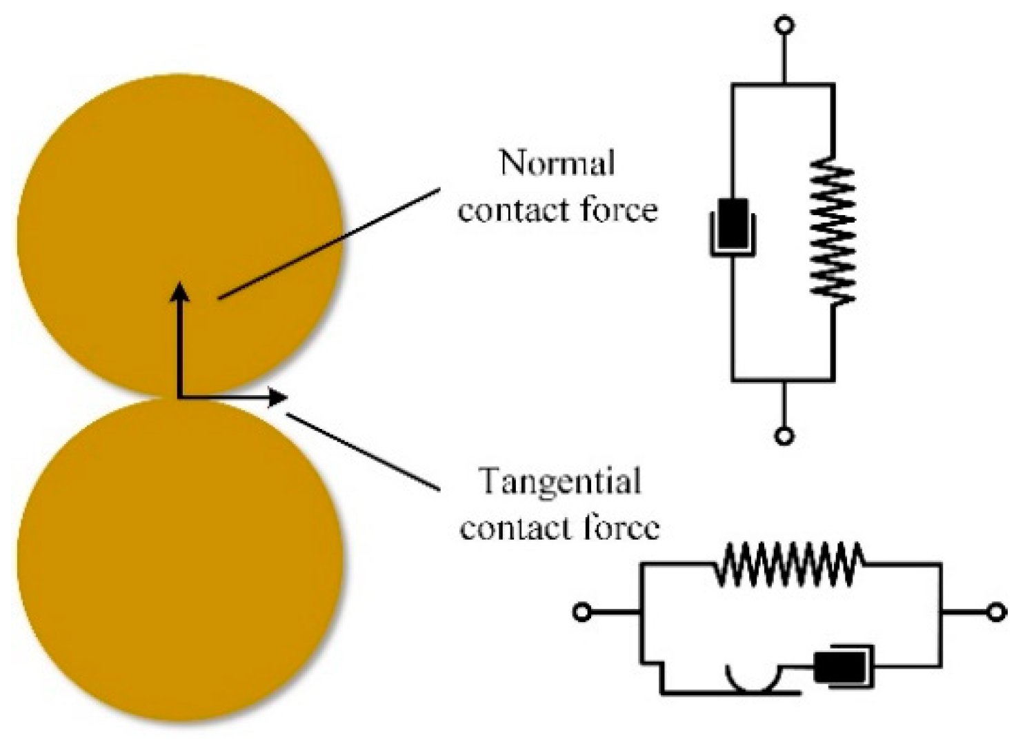
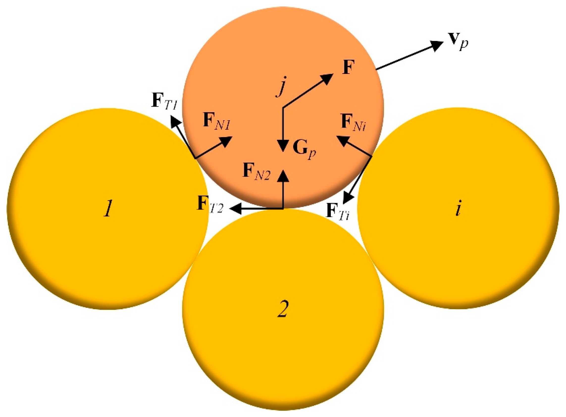
2.2. DEM Model
2.3. Water–Sand Interaction Model
3. Establishment of Local Scour Model
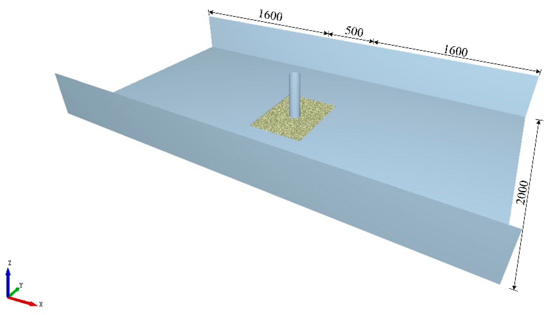
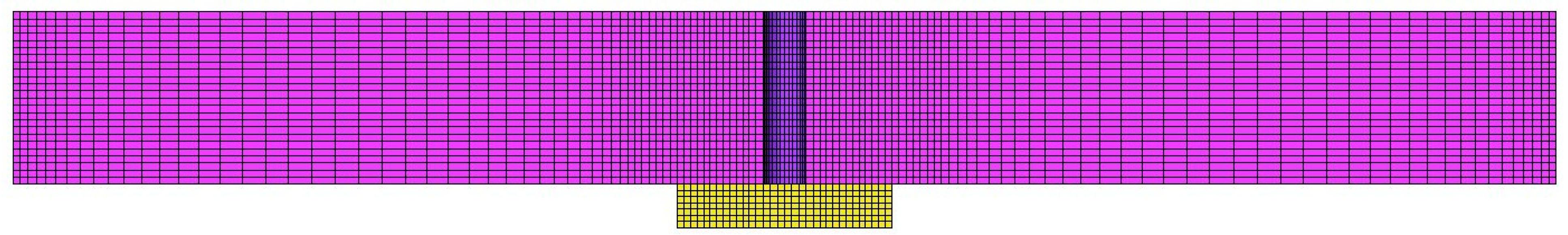
3.1. Geometric Model and Grid Partition
3.2. Setting of Simulation Parameters
3.2.1. EDEM Parameters
3.2.2. Fluent Parameters
3.3. Fluent-EDEM Coupling
4. Analysis and Discussion
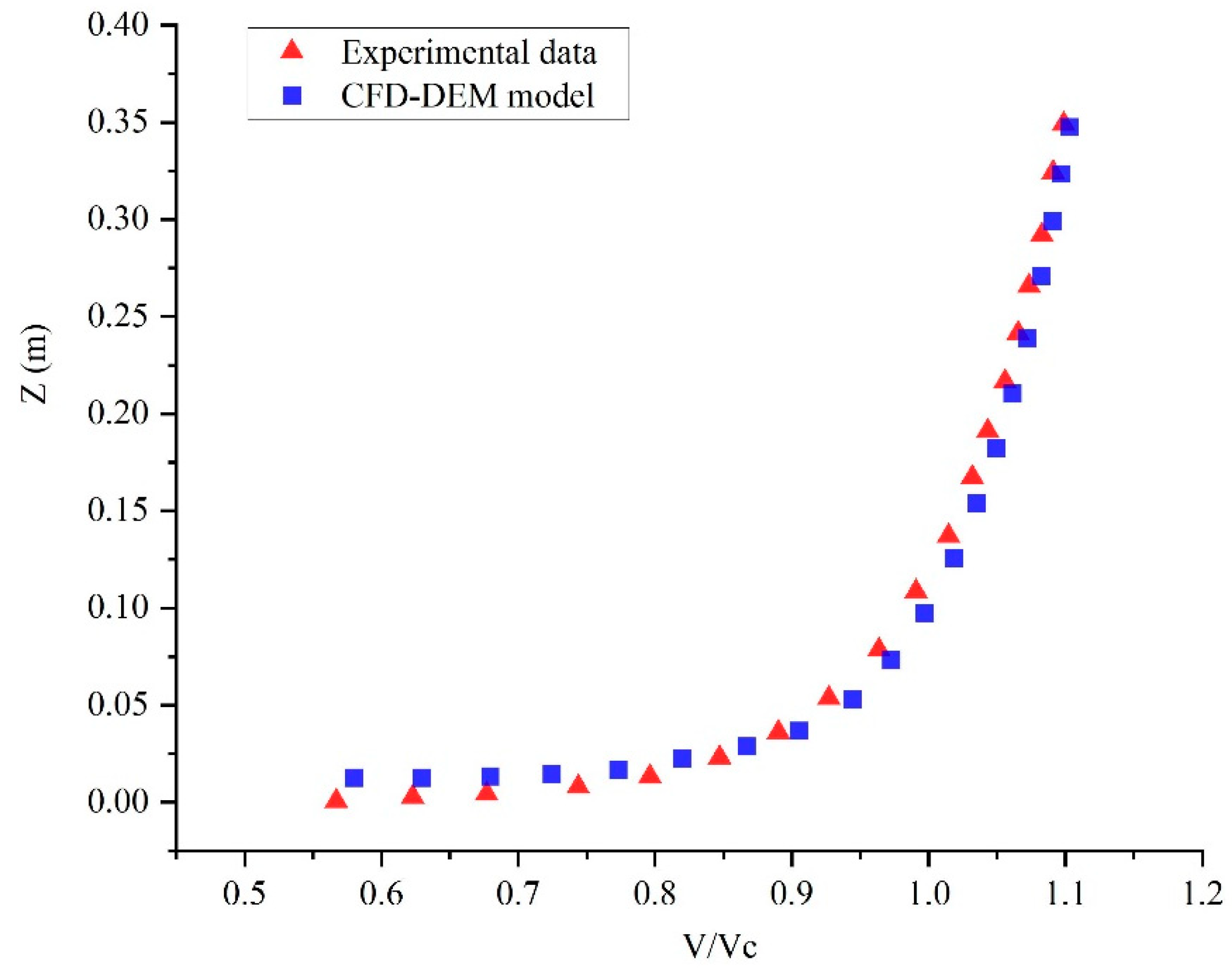
4.1. CFD-DEM Model Verification
4.1.1. Velocity Distribution
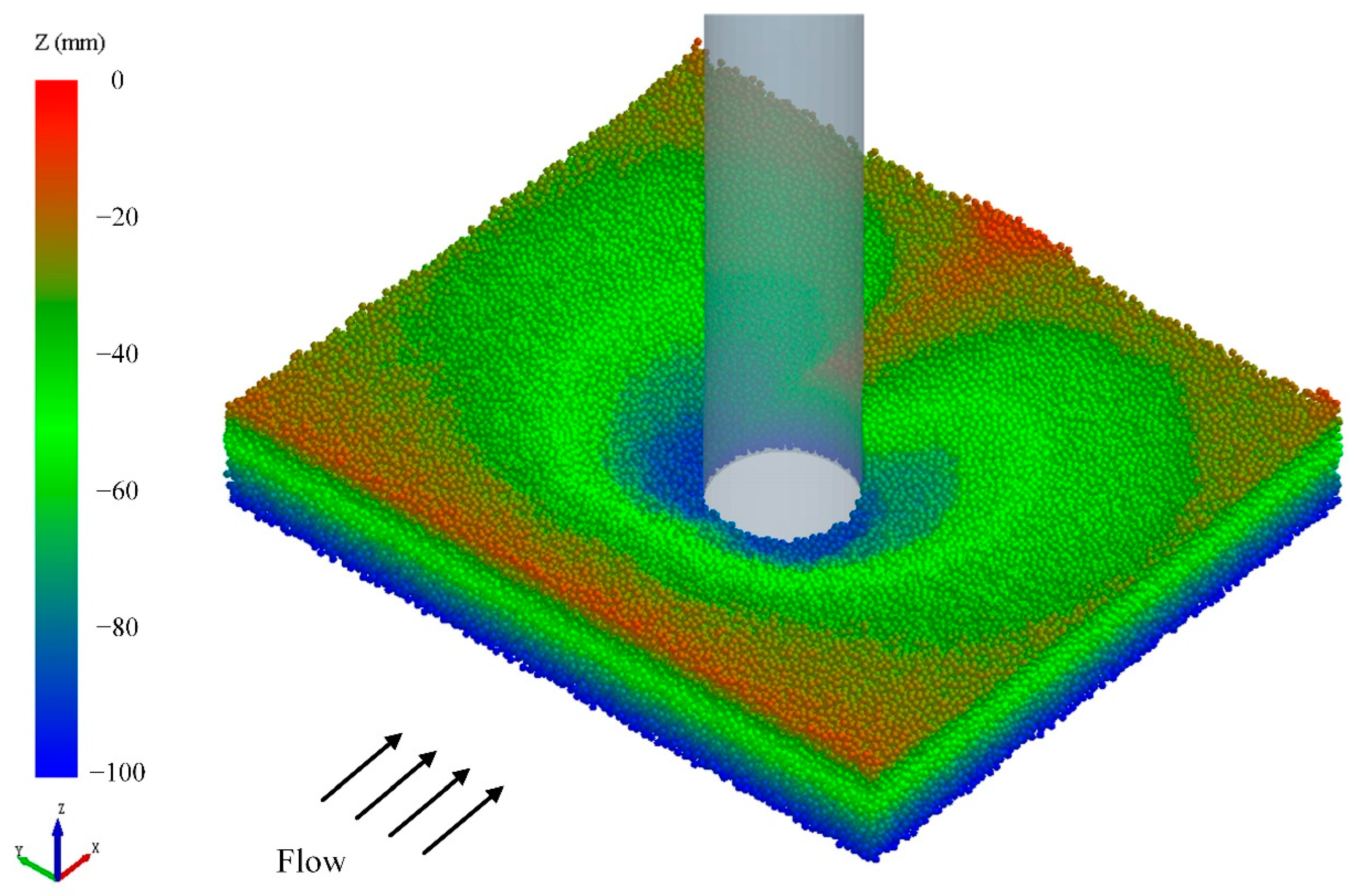
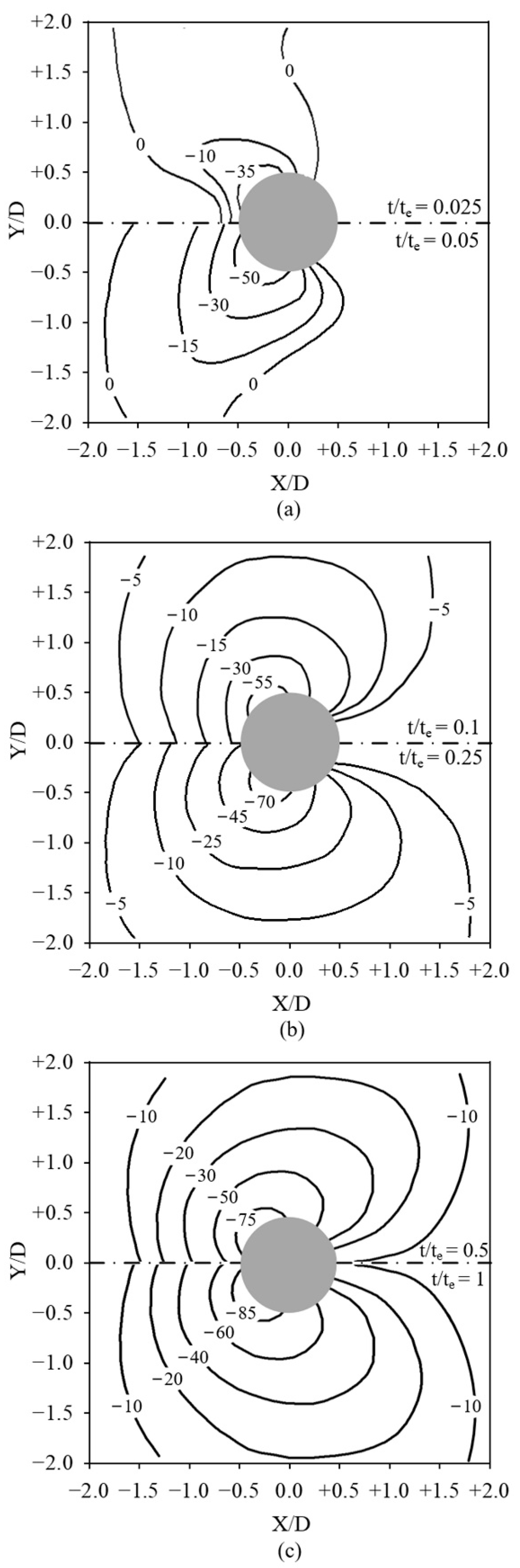
4.1.2. Scour Pit Morphology
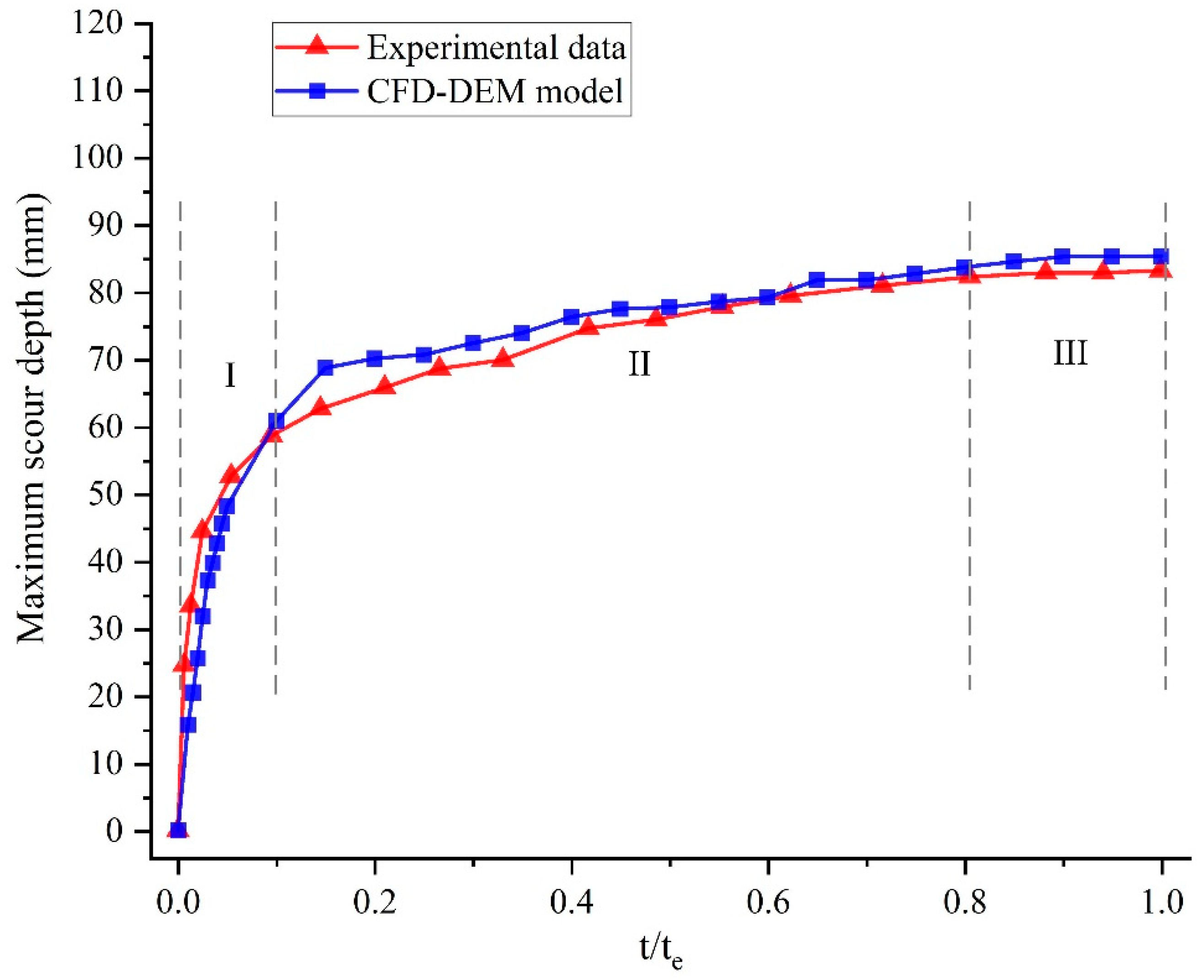
4.1.3. Time History
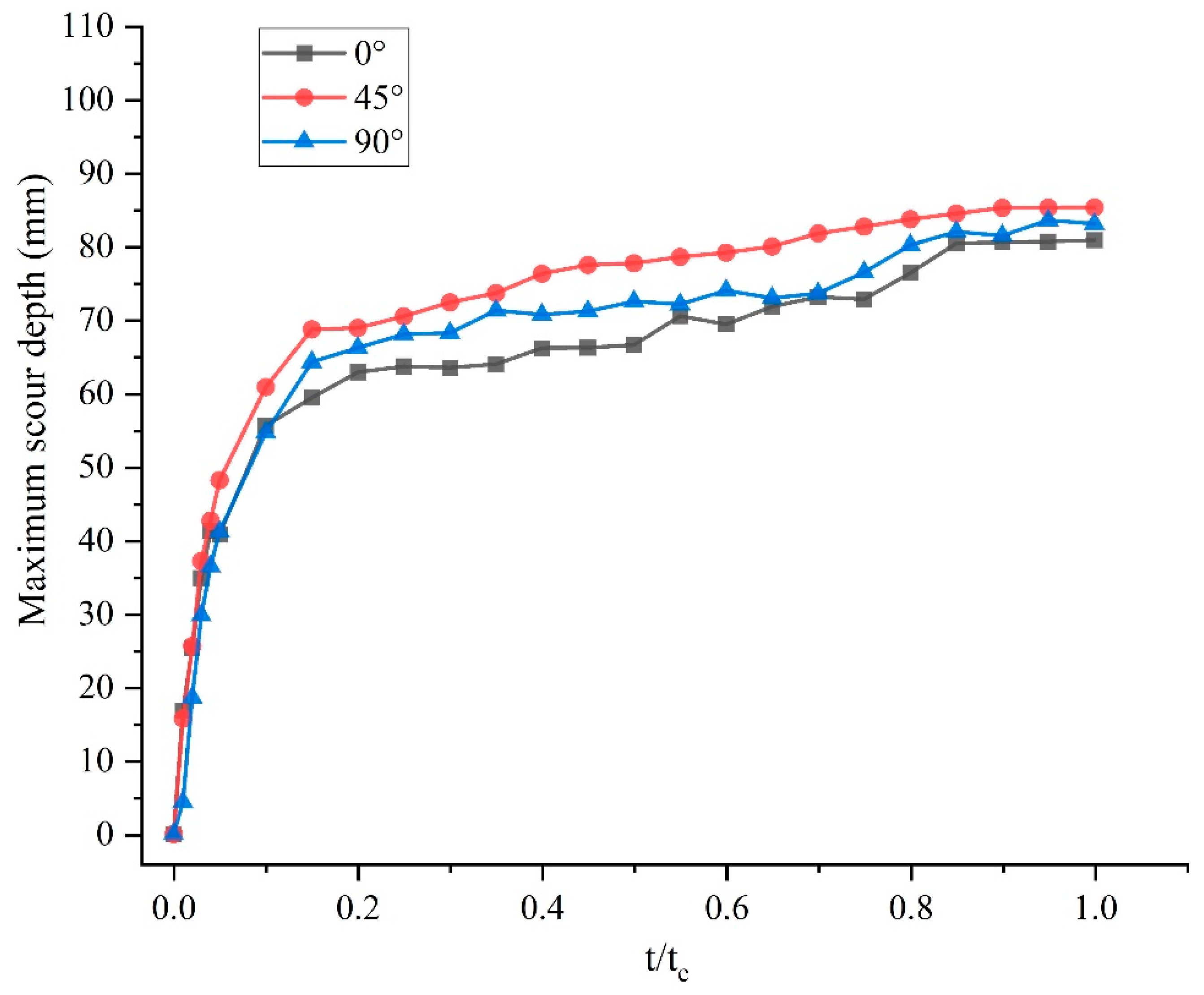
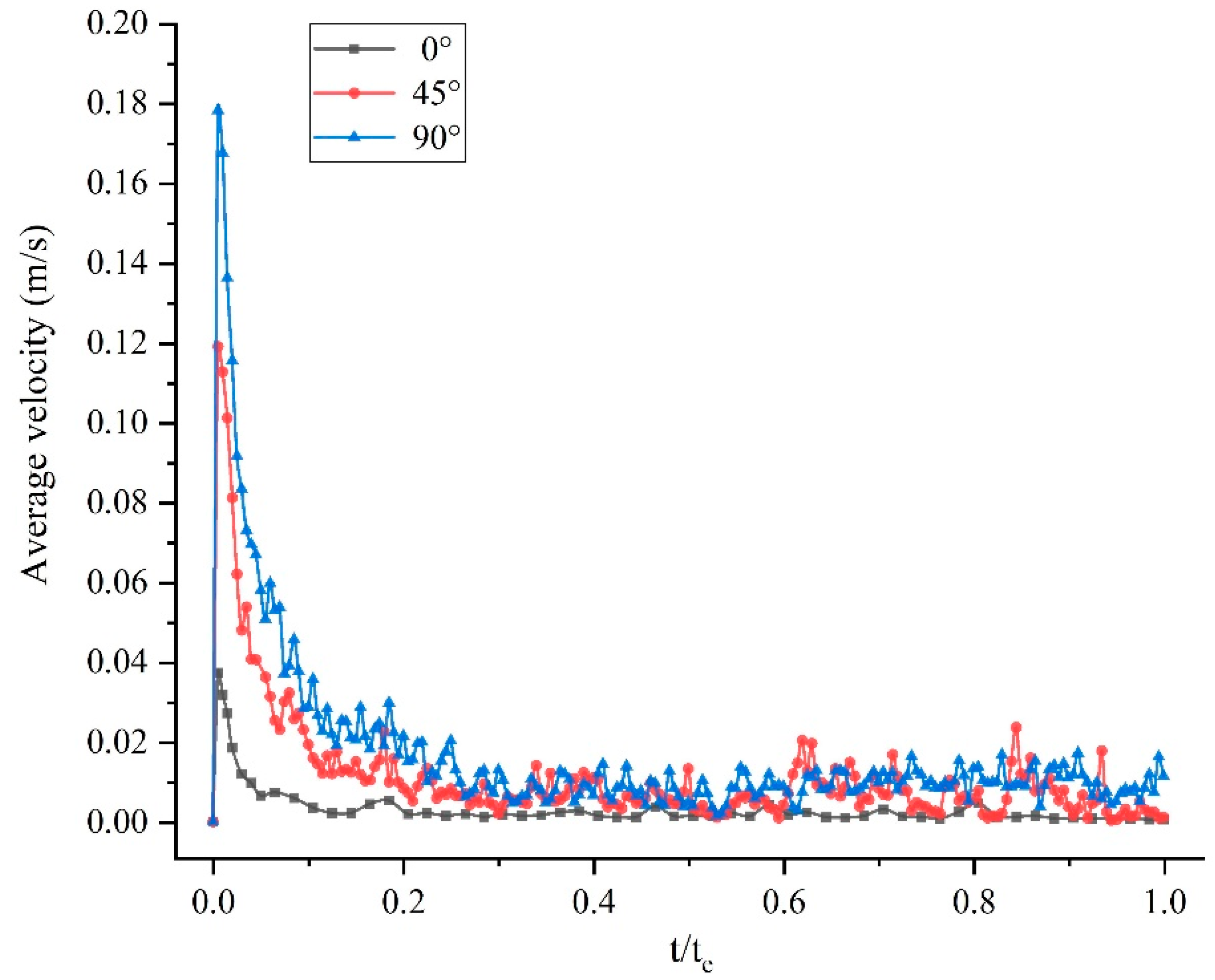
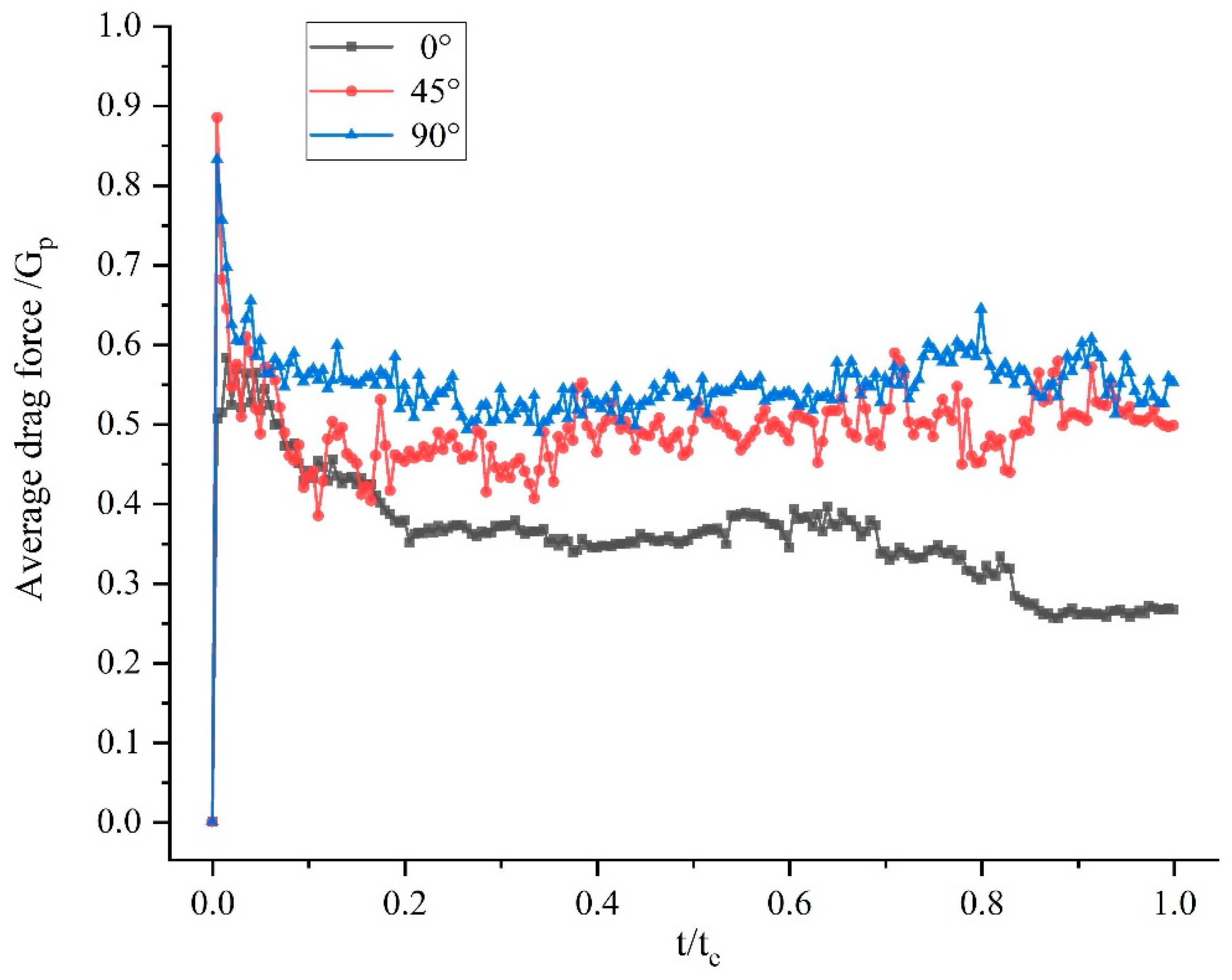
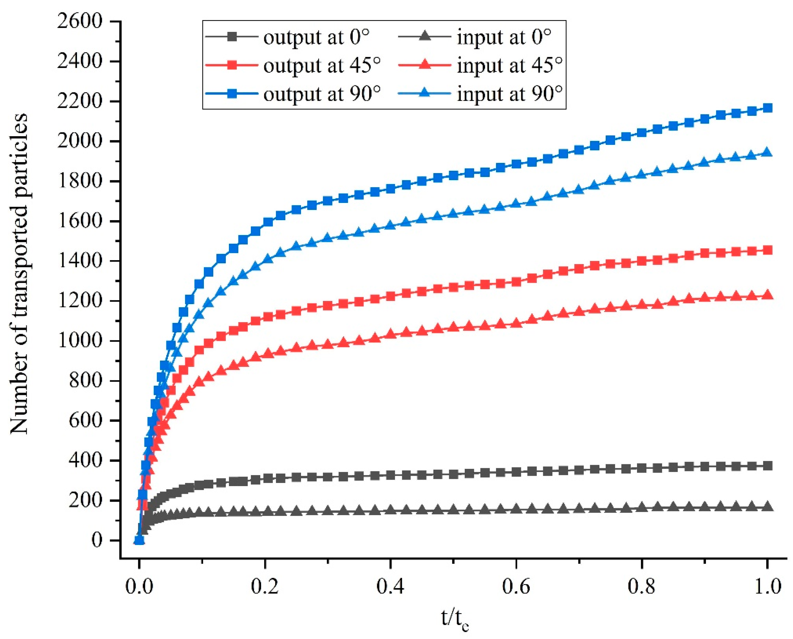
4.2. Macro Scour in Areas around Piles
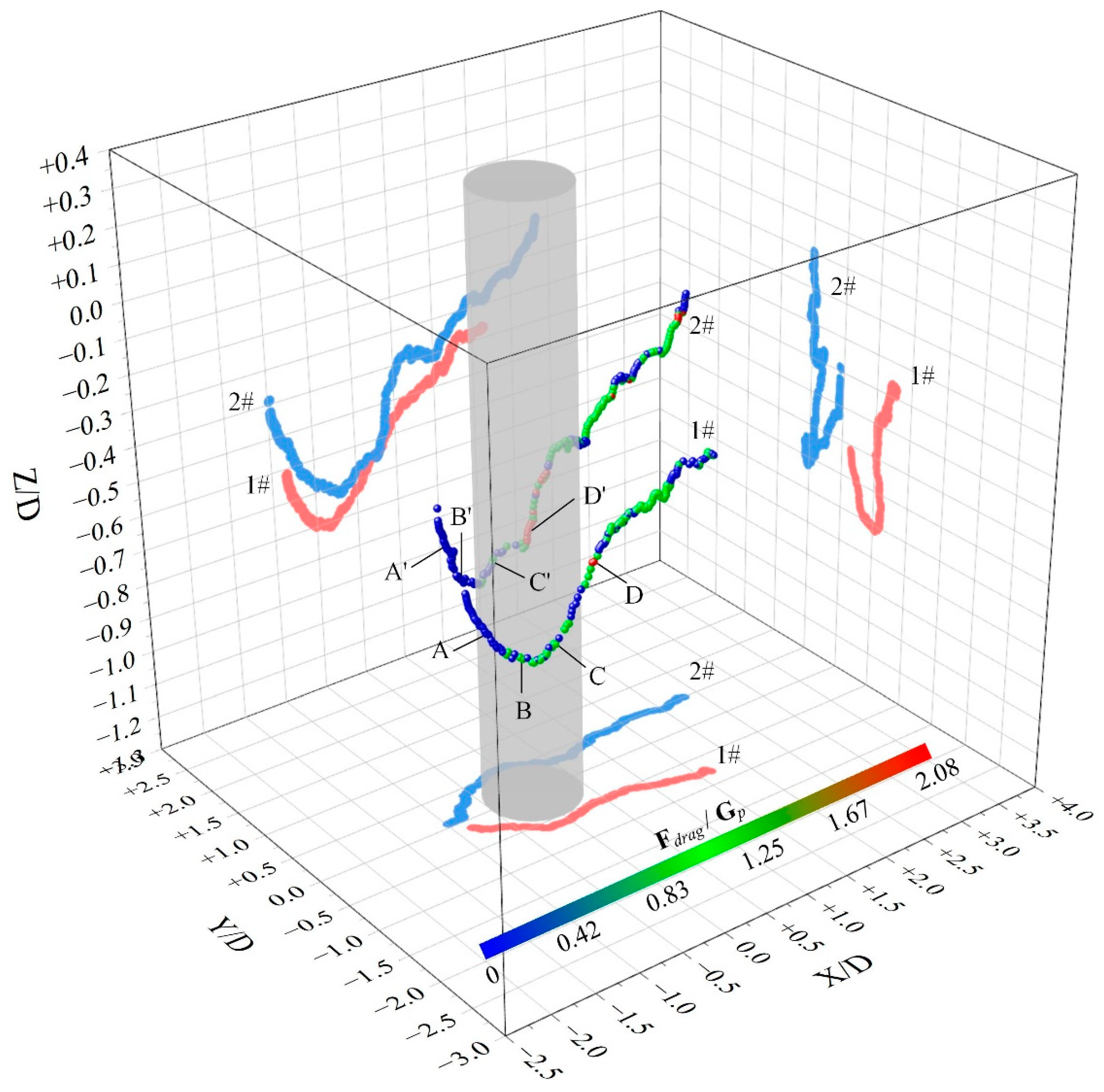
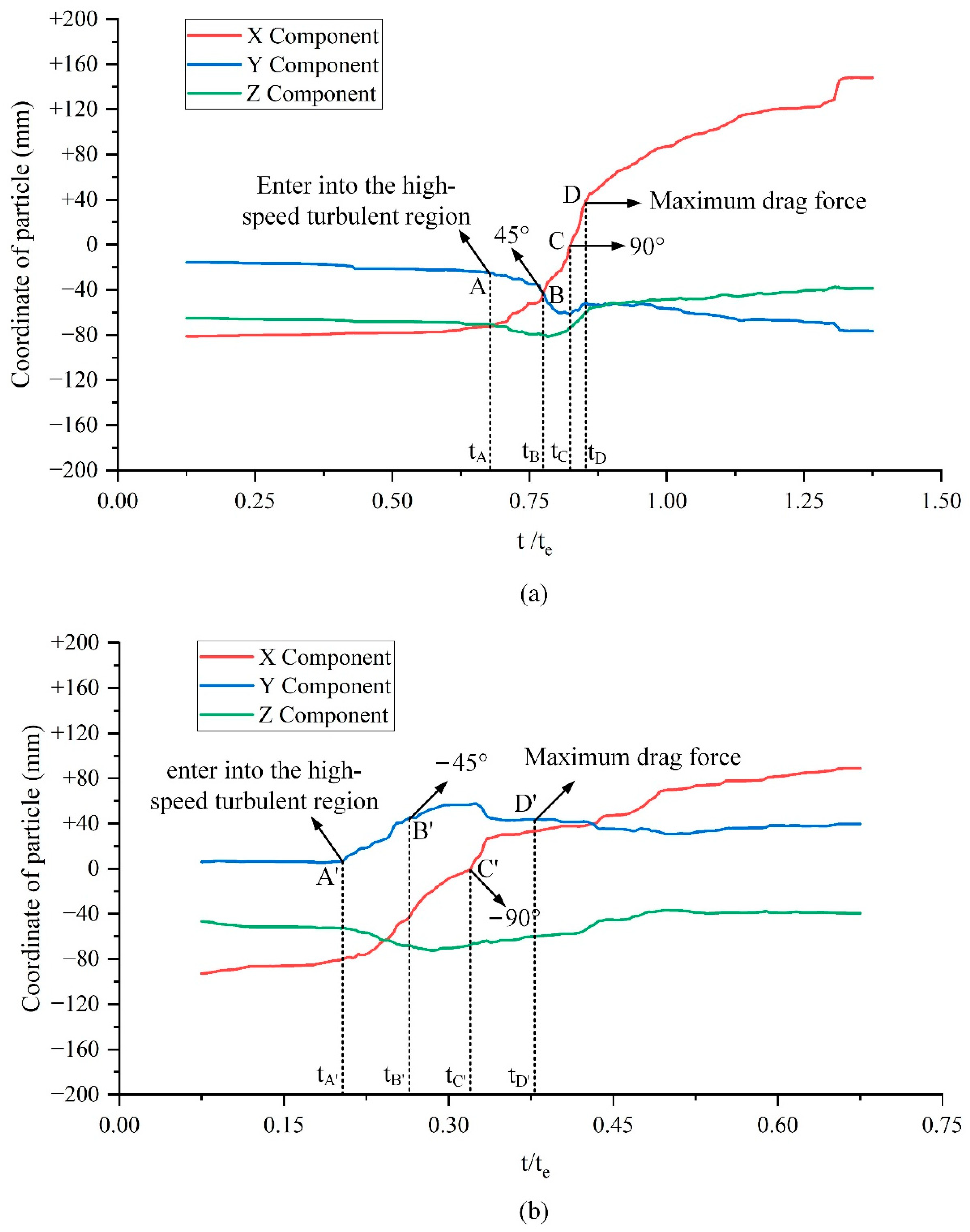
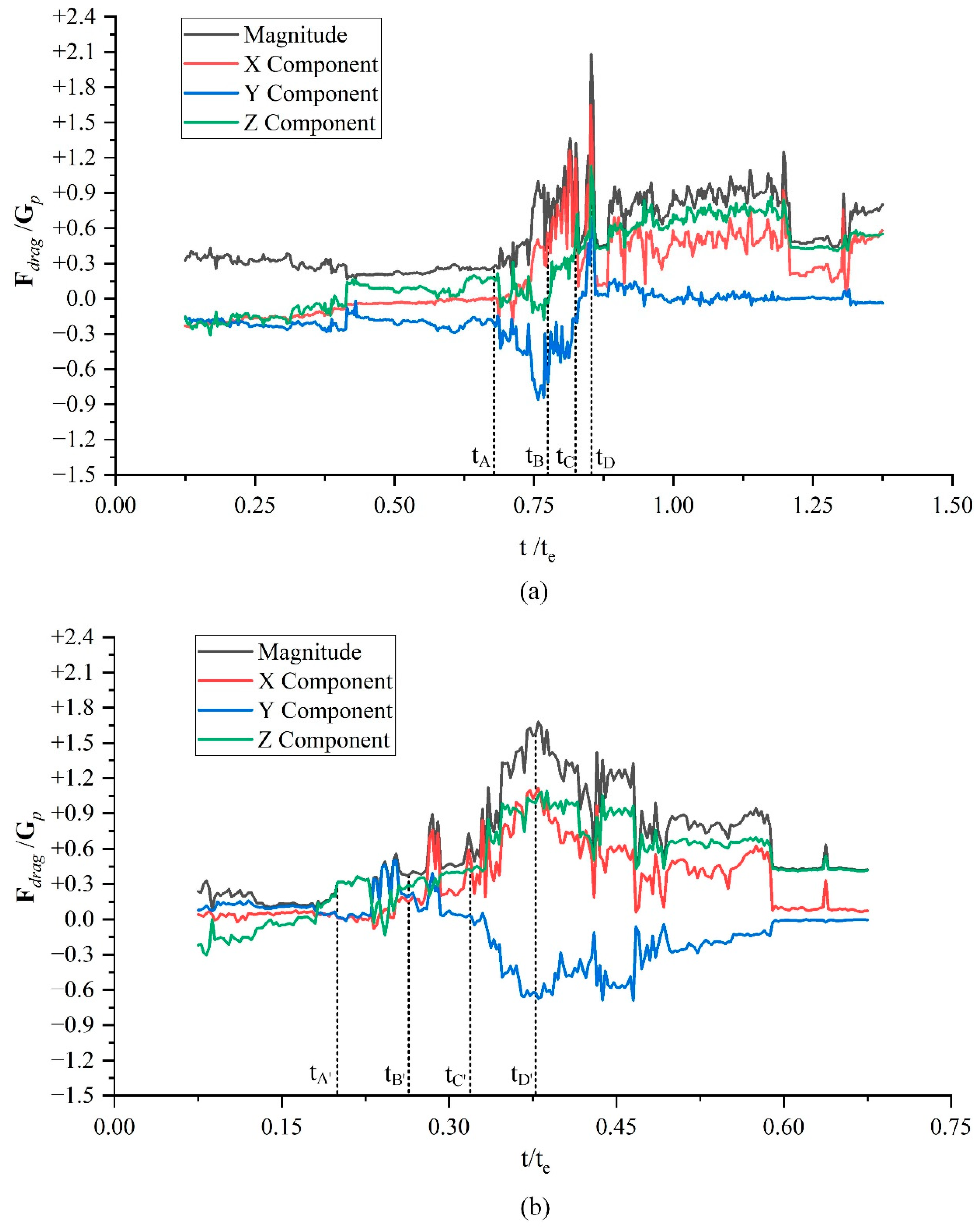
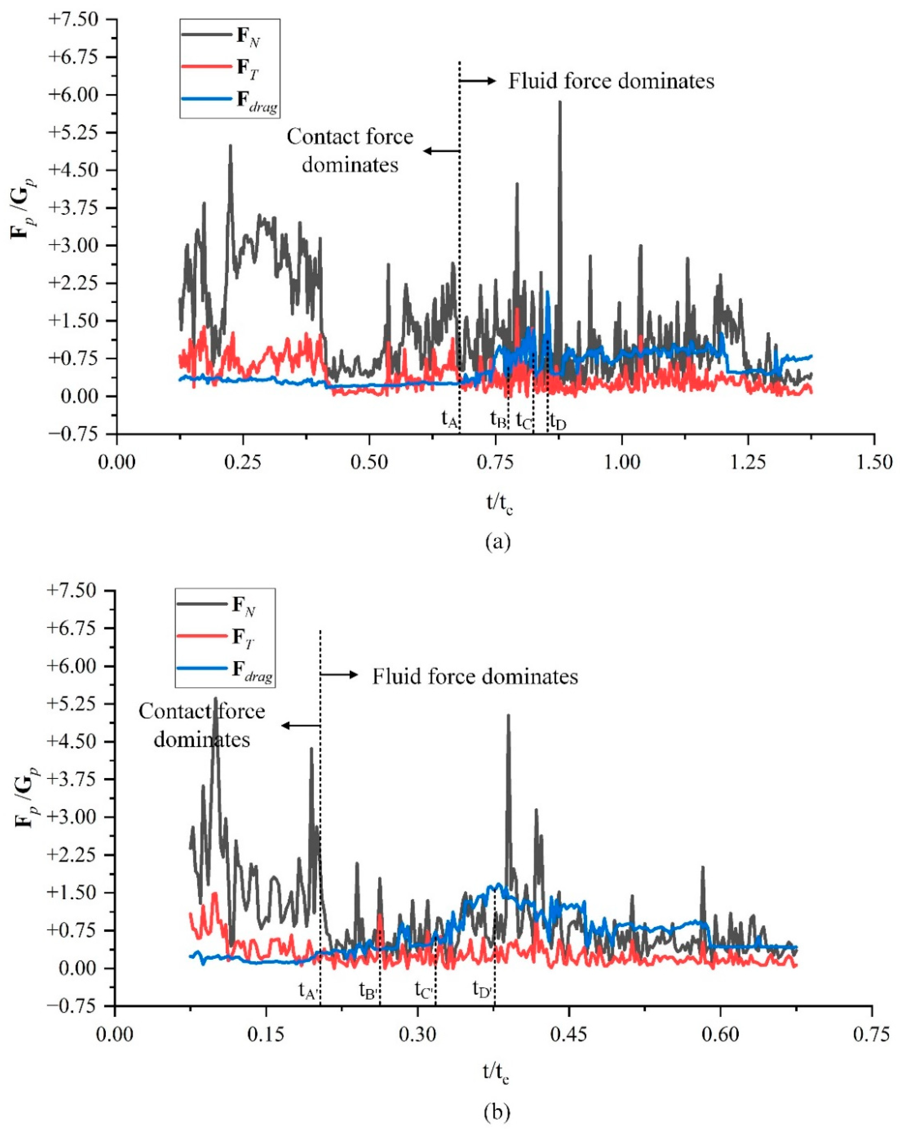
4.3. Mesoscopic Erosion at the Particle Scale
4.4. Discussion of CFD-DEM
4.4.1. Advantages of CFD-DEM
4.4.2. Limits of CFD-DEM
5. Conclusions
Author Contributions
Funding
Institutional Review Board Statement
Informed Consent Statement
Data Availability Statement
Conflicts of Interest
Nomenclature
| Cμ | Empirical constant |
| C1 | Empirical constant |
| C2 | Empirical constant |
| CD | Drag coefficient |
| dp | Particle diameter, m |
| d50 | Median particle size of sediment, m |
| D* | Dimensionless diameter of sediment |
| e | Collision recovery coefficient of particles |
| E* | Equivalent Young’s modulus of particles, Pa |
| Ei | Young’s modulus of the ith particle, Pa |
| f | Momentum transferred by the fluid contained in the unit volume grid to all particles in the grid cell, N/m3 |
| fb | Momentum transfer of fluid contained in unit volume grid to all particles in grid cell due to buoyancy, N/m3 |
| fd | Momentum transfer of fluid contained in unit volume grid to all particles in grid cell due to drag, N/m3 |
| F | Fluid force on particles, N |
| Fdrag | Drag force on particles, N |
| Fdrag,0° | Average drag force on particles at 0° around the pile, N |
| Fdrag,45° | Average drag force on particles at 45° around the pile, N |
| Fdrag,90° | Average drag force on particles at 90° around the pile, N |
| Fdrag,x | X component of the drag force, N |
| Fdrag,y | Y component of the drag force, N |
| Fdrag,z | Z component of the drag force, N |
| Normal damping force on particles, N | |
| Normal contact force amplitude on particles, N | |
| FNi | Normal contact force from the ith particle, N |
| Fp | Total force on particles, N |
| Fp,x | X component of the forces on particle, N |
| Fp,y | Y component of the forces on particle, N |
| Fp,z | Z component of the forces on particle, N |
| FT | Tangential contact forces on particles from particles and geometry, N |
| Tangential damping force on particles, N | |
| Tangential contact force amplitude on particles, N | |
| FTi | Tangential contact force from the ith particle, N |
| g | Gravitational acceleration, m/s2 |
| G* | Equivalent shear modulus of particles, Pa |
| Gp | Weight of sediment, N |
| h | Depth of water, m |
| i | Unit vector in X direction |
| j | Unit vector in Y direction |
| Ip | Moment of inertia of particles, kg·m2 |
| k | Turbulent kinetic energy, m2/s2 |
| k | Unit vector in Z direction |
| Kfp | Fluid–particle momentum exchange coefficient |
| Mass of the ith particle, kg | |
| mp | Particle mass, kg |
| m* | Equivalent mass of particles, kg |
| Mp | Total torque on particles, N·m |
| nc | Number of the sediment particles in contact |
| n | Normal unit vectors |
| p | Hydrostatic pressure, Pa |
| Pk | Generic term of turbulent kinetic energy, kg/(m·s3) |
| R | Distance from the contact point to the centre of mass, m |
| R* | Equivalent radius of particles, m |
| Rep | Relative Reynolds number of particles |
| Ri | Radius of the ith particle, m |
| s | Critical moving direction vector |
| s | Ratio of sediment particle density to water density |
| S | Scour depth, m |
| S0° | Scour depth at 0° around the pile, m |
| S45° | Scour depth at 45° around the pile, m |
| S90° | Scour depth at 90° around the pile, m |
| SN | Normal stiffness of particles, Pa·m |
| ST | Tangential stiffness of particles, Pa·m |
| t | Time, s |
| t | Tangential unit vectors |
| te | Time corresponding to the local scour equilibrium, s |
| Instantaneous velocity of the fluid, m/s | |
| Velocity of particles, m/s | |
| ν | Kinematic viscosity of water, m2·s |
| Normal components of relative velocity of particles, m/s | |
| Tangential components of relative velocity of particles, m/s | |
| Vcell | Grid cell volume, m3 |
| V | Average velocity of water flow along the depth of the water, m/s |
| Vaverage,0° | Average velocity of particles at 0° around the pile, m/s |
| Vaverage,45° | Average velocity of particles at 45° around the pile, m/s |
| Vaverage,90° | Average velocity of particles at 90° around the pile, m/s |
| Vc | Critical starting flow velocity, m/s |
| Vtransport,0° | Sediment transport velocity at 0° around the pile, m/s |
| Vtransport,45° | Sediment transport velocity at 45° around the pile, m/s |
| Vtransport,90° | Sediment transport velocity at 90° around the pile, m/s |
| Greek | |
| Volume fraction of the fluid | |
| αp | Volume fraction of particles |
| ε | Turbulent dissipation rate, m2/s3 |
| Prandtl number corresponding to turbulent kinetic energy | |
| Prandtl number corresponding to turbulent kinetic energy dissipation rate | |
| Normal overlap between contact particles, m | |
| Tangential overlap between contact particles, m | |
| θ | Shields number |
| θcr | Critical shields number |
| κ | Carmen coefficient |
| Fluid density, kg/m3 | |
| ρp | Particle density, kg/m3 |
| Fluid stress tensor, Pa | |
| τs | Shear force of water flow near the bed surface, Pa |
| μ | Hydrodynamic viscosity coefficient, Pa·s |
| Rolling friction coefficients of particles | |
| Sliding friction coefficients of particles | |
| Vorticity coefficient, Pa·s | |
| Poisson’s ratio of the ith particle | |
| Interphase force distribution coefficient of the ith particle in the grid cell | |
| Rotational angular velocity of particles, rad/s |
References
- de la Torre, O.; Hann, M.; Miles, J.; Stripling, S.; Greaves, D. Effect of the current-wave angle on the local scour around circular piles. J. Waterw. Port. Coast. Ocean. Eng. 2022, 148, 04021039. [Google Scholar] [CrossRef]
- Wang, X.; Cheng, Y.; Luo, W.; Huang, X.; Lv, X. Experimental study of local scour and flow field alteration around an inclined pile in steady currents. Period. Ocean. Univ. China 2022, 52, 131–138. [Google Scholar]
- Hu, R.; Wang, X.; Liu, H.; Chen, D. Numerical Study of Local Scour around Tripod Foundation in Random Waves. J. Mar. Sci. Eng. 2022, 10, 475. [Google Scholar] [CrossRef]
- Vonkeman, J.K.; Basson, G.R.; Smit, G.J.F. Hydro-morphodynamic model with immersed boundary method for local scour at bridge piers. ISH J. Hydraul. Eng. 2022, 28, 163–173. [Google Scholar] [CrossRef]
- Melville, B.W. Scour at various hydraulic structures: Sluice gates, submerged bridges and low weirs. Aus. J. Water Resour. 2014, 18, 101–117. [Google Scholar]
- Ma, L.; Wang, L.; Guo, Z.; Jiang, H.; Gao, Y. Time development of scour around pile groups in tidal currents. Ocean Eng. 2018, 163, 400–418. [Google Scholar] [CrossRef]
- Aksoy, A.O.; Bombar, G.; Arkis, T.; Guney, M.S. Study of the time-dependent clear water scour around circular bridge piers. J. Hydrol. Hydromech. 2017, 65, 26–34. [Google Scholar] [CrossRef] [Green Version]
- Fakhari, Z.; Kabiri-Samani, A. Scour in the transition from super- to subcritical flow without a hydraulic jump. J. Hydraul. Res. 2017, 55, 470–479. [Google Scholar] [CrossRef]
- Yang, F.; Qu, L.; Tang, G.; Lu, L. Local scour around a porous surface-piercing square monopile in steady current. Ocean Eng. 2021, 223, 108716. [Google Scholar] [CrossRef]
- Yang, F.; Qu, L.; Zhang, Q.; Tang, G.; Liang, B. Local scour around tandem square porous piles in steady current. Ocean Eng. 2021, 236, 109554. [Google Scholar] [CrossRef]
- Wang, S.; Wei, K.; Shen, Z.; Xiang, Q. Experimental Investigation of Local Scour Protection for Cylindrical Bridge Piers Using Anti-Scour Collars. Water 2019, 11, 1515. [Google Scholar] [CrossRef] [Green Version]
- Bozkuş, Z.; Özalp, M.C.; Dinçer, A.E. Effect of Pier Inclination Angle on Local Scour Depth Around Bridge Pier Groups. Arab. J. Sci. Eng. 2018, 43, 5413–5421. [Google Scholar] [CrossRef]
- Qi, W.G.; Li, Y.X.; Xu, K.; Gao, F.P. Physical modelling of local scour at twin piles under combined waves and current. Coast. Eng. 2019, 143, 63–75. [Google Scholar] [CrossRef] [Green Version]
- Wang, H.; Tang, H.; Liu, Q.; Zhao, X. Topographic Evolution around Twin Piers in a Tandem Arrangement. KSCE J. Civ. Eng. 2019, 23, 2889–2897. [Google Scholar] [CrossRef]
- Jia, Y.; Altinakar, M.; Guney, M.S. Three-dimensional numerical simulations of local scouring around bridge piers. J. Hydraul. Res. 2018, 56, 351–366. [Google Scholar] [CrossRef]
- Wang, Z.; Liu, H.; Yang, Q.; Zhao, Z.; Hu, R. Local scour of large diameter monopile under combined waves and currents. Rock Soil Mech. 2021, 42, 1178–1185+1199. (In Chinese) [Google Scholar]
- Ahmad, N.; Kamath, A.; Bihs, H. 3D numerical modelling of scour around a jacket structure with dynamic free surface capturing. Ocean Eng. 2020, 200, 107104. [Google Scholar] [CrossRef]
- Fan, F.; Liang, B.; Bai, Y.; Zhu, Z.; Zhu, Y. Numerical modeling of local scour around hydraulic structure in sandy beds by dynamic mesh method. J. Ocean Univ. China 2017, 16, 738–746. [Google Scholar] [CrossRef]
- Yu, P.; Zhu, L. Numerical simulation of local scour around bridge piers using novel inlet turbulent boundary conditions. Ocean Eng. 2020, 218, 108166. [Google Scholar] [CrossRef]
- Bhat, N.U.H.; Pahar, G. Euler–Lagrange framework for deformation of granular media coupled with the ambient fluid flow. Appl. Ocean Res. 2021, 116, 102857. [Google Scholar] [CrossRef]
- Kuang, S.; Zhou, M.; Yu, A. CFD-DEM modelling and simulation of pneumatic conveying: A review. Powder Technol. 2020, 365, 186–207. [Google Scholar] [CrossRef]
- Li, J.; Tao, J. CFD-DEM Two-Way Coupled Numerical Simulation of Bridge Local Scour Behavior under Clear-Water Conditions. Transp. Res. Rec. 2018, 2672, 107–117. [Google Scholar] [CrossRef]
- Dai, Y.; Zhang, Y.; Li, X. Numerical and experimental investigations on pipeline internal solid-liquid mixed fluid for deep ocean mining. Ocean Eng. 2021, 220, 108411. [Google Scholar] [CrossRef]
- Chen, Q.; Xiong, T.; Zhang, X.; Jiang, P. Study of the hydraulic transport of non-spherical particles in a pipeline based on the CFD-DEM. Eng. Appl. Comput. Fluid Mech. 2020, 14, 53–69. [Google Scholar] [CrossRef]
- Zhang, Y.; Zhao, M.; Kwok, K.; Liu, M. Computational fluid dynamics-discrete element method analysis of the onset of scour around subsea pipelines. Appl. Math. Model. 2015, 39, 7611–7619. [Google Scholar] [CrossRef]
- Hu, D.; Tang, W.; Sun, L.; Li, F.; Ji, X.; Duan, Z. Numerical simulation of local scour around two pipelines in tandem using CFD–DEM method. Appl. Ocean Res. 2019, 93, 101968. [Google Scholar] [CrossRef]
- Yang, J.; Low, Y.M.; Lee, C.-H.; Chiew, Y.-M. Numerical simulation of scour around a submarine pipeline using computational fluid dynamics and discrete element method. Appl. Math. Model. 2018, 55, 400–416. [Google Scholar] [CrossRef]
- Ma, H.; Zhao, Y.; Cheng, Y. CFD-DEM modeling of rod-like particles in a fluidized bed with complex geometry. Powder Technol. 2019, 344, 673–683. [Google Scholar] [CrossRef]
- Wang, Z.; Liu, M. Semi-resolved CFD-DEM for thermal particulate flows with applications to fluidized beds. Int. J. Heat Mass Transf. 2020, 159, 120150. [Google Scholar] [CrossRef]
- Launder, B.E.; Spalding, D.B. Lectures in Mathematical Models of Turbulence; Academic Press: London, UK, 1972. [Google Scholar]
- Mindlin, R.D.; Deresiewicz, H. Elastic Spheres in Contact Under Varying Oblique Forces. J. Appl. Mech. 2021, 20, 327–344. [Google Scholar] [CrossRef]
- Gidaspow, D.; Bezburuah, R.; Ding, J. Hydrodynamics of Circulating Fluidized Beds: Kinetic Theory Approach. In Fluidization VII, Proceedings of the 7th Engineering Foundation Conferenceon Fluidization; Illinois Institute of Technology: Chicago, IL, USA, 1992; pp. 75–82. [Google Scholar]
- Crowe, C.T.; Schwarzkopf, J.D.; Sommerfeld, M.; Tsuji, Y. Multiphase Flows with Droplets and Particles; CRC Press: Boca Raton, FL, USA, 1998. [Google Scholar]
- Li, C.A.; Ahmadi, G. Dispersion and deposition of spherical particles from point sources in a turbulent channel flow. Aerosol Sci. Technol. 1992, 16, 209–226. [Google Scholar] [CrossRef]
- Sawaragi, T.; Deguchi, I. Waves on Permeable Layers. Int. Conf. Coastal. Eng. 1992, 1. [Google Scholar] [CrossRef]
- Chen, L.; Zheng, D.; Wang, P.; Zhu, B. Analysis of wave force acting on the monopile based on wave-porous seabed-structure coupled model. Eng. Mech. 2019, 36, 72–82. (In Chinese) [Google Scholar]
- Liu, D.; Fu, X.; Wang, G. Volume fraction allocation using characteristic points for coupled CFD-DEM calculations. J. Tsinghua Univ. (Sci. Technol.) 2017, 57, 720–727. (In Chinese) [Google Scholar]
- Wang, D.; Wang, Y.; Yang, B.; Zhang, W. Statistical analysis of sand grain/bed collision process recorded by high-speed digital camera. Sedimentology 2008, 55, 461–470. [Google Scholar] [CrossRef]
- Xu, Y. Experimental Investigation of Scour around Vertical Piles in Steady Currents; Dalian University of Technology: Dalian, China, 2018. (In Chinese) [Google Scholar]
- Zhao, M.; Cheng, L.; Zang, Z. Experimental and numerical investigation of local scour around a submerged vertical circular cylinder in steady currents. Coast. Eng. 2010, 57, 709–721. [Google Scholar] [CrossRef]
- Guo, J.; Wang, T.; Wang, J.; Wu, J. Calculation of local scour depth of steel pipe pile for sea-crossing bridge based on energy balance theory. Ocean. Eng. 2020, 38, 96–106. (In Chinese) [Google Scholar]


| Parameter | V1D3 Test [39] | CFD-DEM |
|---|---|---|
| Pile foundation diameter D (m) | 0.1 | 0.1 |
| Average flow velocity V (m/s) | 0.286 | 0.92 |
| Water depth h (m) | 0.4 | 0.4 |
| Median sediment particle size d50 (mm) | 0.29 | 5 |
| Natural angle of repose of sediments (°) | 33 | 33 |
| Shields number θ | 0.035 | 0.048 |
| Critical Shields number θcr | 0.038 | 0.052 |
| θ/θcr | 0.92 | 0.92 |
Publisher’s Note: MDPI stays neutral with regard to jurisdictional claims in published maps and institutional affiliations. |
© 2022 by the authors. Licensee MDPI, Basel, Switzerland. This article is an open access article distributed under the terms and conditions of the Creative Commons Attribution (CC BY) license (https://creativecommons.org/licenses/by/4.0/).
Share and Cite
Liu, Q.; Wang, Z.; Zhang, N.; Zhao, H.; Liu, L.; Huang, K.; Chen, X. Local Scour Mechanism of Offshore Wind Power Pile Foundation Based on CFD-DEM. J. Mar. Sci. Eng. 2022, 10, 1724. https://doi.org/10.3390/jmse10111724
Liu Q, Wang Z, Zhang N, Zhao H, Liu L, Huang K, Chen X. Local Scour Mechanism of Offshore Wind Power Pile Foundation Based on CFD-DEM. Journal of Marine Science and Engineering. 2022; 10(11):1724. https://doi.org/10.3390/jmse10111724
Chicago/Turabian StyleLiu, Qin, Zhe Wang, Ning Zhang, Hongyu Zhao, Lei Liu, Kunpeng Huang, and Xuguang Chen. 2022. "Local Scour Mechanism of Offshore Wind Power Pile Foundation Based on CFD-DEM" Journal of Marine Science and Engineering 10, no. 11: 1724. https://doi.org/10.3390/jmse10111724
APA StyleLiu, Q., Wang, Z., Zhang, N., Zhao, H., Liu, L., Huang, K., & Chen, X. (2022). Local Scour Mechanism of Offshore Wind Power Pile Foundation Based on CFD-DEM. Journal of Marine Science and Engineering, 10(11), 1724. https://doi.org/10.3390/jmse10111724