Article

Using Different Classic Turbulence Closure Models to Assess Salt and Temperature Modelling in a Lagunar System: A Sensitivity Study

by
José Fortes Lopes
CESAM, Departamento de Física, Universidade de Aveiro, 3810-193 Aveiro, Portugal
J. Mar. Sci. Eng. 2022, 10(11), 1750; https://doi.org/10.3390/jmse10111750
Submission received: 11 October 2022 / Revised: 1 November 2022 / Accepted: 8 November 2022 / Published: 14 November 2022

Abstract

:
Turbulence modelling is an important issue when dealing with hydrodynamic and transport models for better simulation of the transport of dissolved or suspended substances in a body-water. It controls processes involving physical balances (salt and water temperature) and, therefore, the ecosystem equilibrium. The study arises from the need to model the turbulence more efficiently when dealing with extreme situations on the Ria de Aveiro (Portugal), a coastal lagoon shallow water system dominated by tidal transport. Because the turbulence model is coupled to the hydrodynamic and transport models, a correct estimation of the eddy viscosity is important in simulating the salt and the heat transports. The aim is to assess the performance of four turbulence schemes/models (k, k-ε, Smagorinsky’s, and k-ε/Smagorinsky’s (k-ε/Sma), where k is turbulent kinetic energy and ε the dissipation rate of the turbulent kinetic energy) associated to a coupled hydrodynamic and transport models to simulate the eddy viscosity, the salinity, and the temperature. Overall, the results point out that among the different models/schemes used, the is the one which provides a more realistic value of the eddy viscosity within the range (1–6) m2 s−1, but most probably (1–3) m2 s−1. The application of the sensitivity analysis to some non-universal k-ε/Sma parameters evidenced significant sensitivity for the eddy viscosity and the salinity and moderate sensitivity for the water temperature. A 100% adjustment of the parameter values relative to the reference, translated into variations within the range of (1, 4) m2 s−1, (0, 13) PSU, and (1, 2.20) °C, for the eddy viscosity, salinity, and water temperature, respectively.

1. Introduction

Turbulence modelling and prediction are crucial in science today. Turbulence covers a wide range of fields, spanning from the general fluid mechanics [1,2,3] to the environmental sciences, dealing with geophysical and astrophysical fluid dynamics [4,5,6,7,8], and the industrial applications, dealing with aerodynamics, energy, transportation, etc. [9,10,11,12].
Turbulence has been studied for nearly a hundred years. Despite numerous experimental and computational advances, it remains an enigmatic topic in fluid mechanics and physics [13]. Among three significant challenges posed by turbulence [13], which are the dynamical closure of the turbulence, the structural scaling, and the energy spectra, the first is the most crucial when dealing with modelling studies. Indeed, the closure of the turbulence allows for determining the turbulent eddy viscosity and diffusion coefficients, which are fundamental parameters for numerically solving the hydrodynamic and the transport equations. The most basic assumption constitutes the so-called mixing length of the Prandtl model [14], which assumes that the fluid flow conserves its macroscopic properties for a characteristic length scale of the flow before mixing with the surrounding fluid. For instance, Rousseau and Ancey [15] managed to capture the mean-velocity and turbulence-intensity profiles of shallow flows over a horizontal or sloping permeable bed by using an algebraic closure equation for dispersive shear stress based on the mixing-length model. Nevertheless, in most complex flows, this type of formulation falls short of capturing the complexity of the turbulence. Another essential formulation is based on the so-called subgrid-scale turbulence closure model, proposed in 1963 by Smagorinsky [16,17], which is still widely used. It is based on the local gradients of the velocity field when the flow has a clearly defined spectral gap, which can be decomposed on the base of large-scales and fine-scales, with moderate and arbitrary gradients. Therefore, the subgrid-scale represents the small-scale below which it is not possible to resolve the turbulence equations on a computational mesh. It requires an understanding of the physics and the statistics of the scale interactions, which is quite an open scientific problem [18]. The eddy viscosity in the Smagorinsky model is, therefore, linked to the grid size and the velocity gradients for the large eddy strain of the resolved flow field. Burman et al. [19] showed that the Smagorinsky model is efficient in situations of high Reynolds number, near rough surface flows, or in geophysical fluid dynamics.
As turbulence is still an open subject, various sophisticated models abound in the literature today and are applied in environmental and industrial fluid flows [20,21]. The most relevant turbulent models in connection with those used in this study are the Reynolds–averaged Navier–Stokes (RANS), the large-eddy simulation (LES), the hybrid RANS/LES, and the scale-adaptive simulation (SAS). RANS is the most classical one. It decomposes the flow variables into mean and fluctuating parts and then averages the equations. In the end, to close the turbulence, the so-called Reynolds-stress tensor is defined [22,23,24]. The LES is a high-resolution turbulence model sensitive to the fine details of the equations and the meshes used to represent the flow [25,26,27,28,29,30]. The SAS introduces the von Karman length scale [31,32,33] to avoid dependency determining of the RANS/LES interface. The k-ε model associated to Launder [34] and Launder and Spalding, 1972, [35,36]), and the k (or k-kl) model associated with the Mellor and Yamada model [31,32,33,34,35,36,37,38,39,40,41], are classical versions of RANS. The first one uses the dynamic equations composed of two-equation turbulence models for the turbulent kinetic energy, k, the turbulent dissipation rate, ε, and a macroscopic length scale of the turbulence, l, combined with an algebraic second-moment closure. The second one only uses a one-equation turbulence model for k, whereas l is prescribed. Both models have been applied independently for years in many situations dealing with engineering or geophysical flows [8,9,41]. Burchard [42] and Burchard et al. [43,44] compared in detail the two models and showed that after modifications of the buoyancy production term suggested by Burchard and Baumert [45] for the k-ε model and Burchard and Bolding 2001 [46] for the k/k-l model, both models are equivalent. A modified version of the Smagorinsky model, called the mixed k-ε/Smagorinsky model, combines the advantage of both models separately while including the vertical buoyancy effect, which was set up in this study. This approach allows the determination of the horizontal eddy viscosity through the Smagorinsky formulation, whereas the vertical eddy viscosity is obtained from the one-dimensional k-ε model. Despite some issues when dealing with strong anisotropic or curve flows, irrotational strains, stagnation flow, and near the boundary layers flow separation points, there are several advantages to using k-ε-based models [47,48,49]. The first one concerns the isotropic eddy viscosity, a simple concept. The second one, and the most important, involves the second-order gradients in the mean-flow equations, which preserve the stability of the model.
So far, few modelling studies have focused on aspects dealing with turbulence modelling for the Ria de Aveiro lagoon, an important issue concerning simulating the transport of dissolved and particulate matter. The turbulence model adopted in this study assumes the following schemes: k, k-ε, and the mixed formulation k-ε/Smagorinsky (k-ε/Sma) [50]. The main goal is to assess their performance in simulating the eddy viscosity, the salinity, and the temperature. The turbulent schemes are set up for the salt and temperature. Some statistical tools will be used, presented in Section 3, which allow an objective assessment of the relative skills of the models.
This article is organized as follows. Section 2 presents the study area where the models are applied. Section 3 presents the models used in the simulations. Section 4 presents the results, and Section 5 the discussion and conclusions.

2. The Study Area

Ria de Aveiro (Figure 1) is a shallow, coastal, and well-mixed lagoon (average depth of 1 m) located on the Northwest Atlantic coast of Portugal (40°38′ N, 8°45′ W) and is connected to the sea through a narrow entrance. Among the four main channels, the Ilhavo, the Mira, S. Jacinto, and the Espinheiro, the latter two are responsible for most saltwater and freshwater exchanges (Figure 1). Two main rivers contribute to the lagoon’s main freshwater supply, the Vouga and the Antuã. They are situated at the eastern boundary of the lagoon, with estimated average flows of up to 50 m3 s−1 and 5 m3 s−1 [24] or 80 m3 s−1 and 20 m3 s−1 [51]. Several other small rivers (the Cáster, the Boco, and the Ribeira dos Moínhos) discharge at the lagoon’s northern and southern boundaries, with average flows below 5 m3 s−1 [52]. During the wet season (spring and autumn), the sudden increase in the river tributaries generates intense river pulses or flash floods. In particular, the Vouga river transient runoff may experience peak discharge of up to 120 m3 s−1 [53]. This value can be doubled in a highly wet and heavy runoff situation.
Due to its shallowness and tidal dominance, the lagoon may be considered vertically homogeneous or well-mixed. In addition, some stratification may occur in the deepest areas near the mouth, close to the ocean boundaries, when inner brackish or warm water meets oceanic salty and cold water [54,55,56]. Despite the lagoon’s well-mixed nature, flow driven by tidal advective processes may induce significant changes in the temperature and salinity patterns. This effect may locally affect the turbulence inside the main areas through the generation of horizontal gradients and local vertical stratification.
In recent decades, the Aveiro coastal area has experienced some episodes of intense precipitation and dryness, reflecting a significant departure from the salinity pattern.
Table 1 displays salinity and temperature values for spring (March 2001) and summer (June 2001). They correspond, respectively, to extreme wet and typical dry seasons. The rainfall reached pick values as high as 757 mm [57,58,59,60]. Although no measurements of the river’s flow were performed during this period, it is plausible that it exceeded the average values several times over, especially for the main river (the Vouga), attesting to the extreme salinity values observed [57,58,59,60]. Indeed, St1, which generally exhibits high salinity values (~34 PSU), experienced a minimum salinity value as low as 6 PSU, whereas the peak value only reached 29 PSU. Similar situations occurred for St2 and St5. Summer corresponds, in general, to a dry season characterized by moderate or low river discharge. Typical summer salinity values, as in June 2001, were in the range of (30–34) PSU (which are values close to the ocean salinity), whereas low values (<5 PSU) were found close to the major river boundaries (stations 3, and 4) or at the far end areas (stations 6, 7 and 8) (30–33) PSU. The water temperature was in the range of (13–18) °C for spring and (18–24) °C for summer, typical values for those seasons.

3. Material and Methods

3.1. The Models

3.1.1. The Transport Model for Salt and Temperature

The model used in this work is the baseline Mike3-HD [50,61], which is based on the numerical solution of the two/three-dimensional incompressible Reynolds-averaged Navier–Stokes equations, subject to the assumptions of Boussinesq and of hydrostatic pressure and consists in a system of continuity, momentum, temperature, and salinity equations. The water density does not depend on the pressure but on the temperature and salinity. The salinity and temperature dispersions are assumed to be proportional to the effective eddy viscosity.
Thus, transport equation for salt, S, and temperature, T, is written in as the material derivative [50,61], using a tensorial condensed notation:
1 ρ D ρ S D t = x j ( ν T σ T S x j )
1 ρ D ρ T D t = x j ( ν T σ T T x j ) + 1 ρ Q H  
where t is the time, xj represents the spatial cartesian coordinates, Q H is the term source for heat, σ T   an empirical constant for the turbulence (corresponding to the Prandtl number), ρ is the water density and ν T the eddy viscosity. The above equations are not closed unless a closure scheme is defined. As referred to in Section 1, ν T is derived from the assumption that the energy is contained in the large-scale eddies, l, which is defined as the mixing length scale of the turbulence. It constitutes an inherent quantity to be prescribed for turbulence closure.
The model domain covers a rectangular area corresponding to 266 × 654 cells, with a resolution of 60 m. The time-step integration is set to 1 s, implying a near-absolute hydrodynamic stability condition. The numerical equations are solved using a vertical σ-transformation σ = (zzb)/h, where z and zb denote the surface and bottom layer elevation, and σ ranges between 0 at the bottom, and 1 at the surface. The hydrodynamic model is set up by spinning up the lagoon from rest. The sea surface elevation (tides) is imposed at the ocean’s western open boundary using the Admiralty method of the MIKE3 tide prediction of height [50]. Initial and open boundary (Dirichlet (or first-type)) conditions, including rivers, for the physical state variables, are set according to data [57,58,59,60]. The interaction with the atmosphere is allowed through the exchange of momentum, heat, and radiation. Therefore, according to the same data, wind speed and direction, air temperature, humidity, incident radiation, and sky clearness are imposed (time step of 15 min) at the surface.

3.1.2. The Turbulence Models

-
The k-l turbulence model
The k turbulence model is a one-equations turbulence model which constitutes an important improvement of the mixing-length theory, where k is the turbulent kinetic energy defined as:
k = 1 2 u i u i ¯
A one-dimension transport equation for k is written as the balance between the advection, the diffusions, the dissipation rate, and the buoyancy density vertical gradients:
k t + u i k x i + x i [ ν T   σ k k x i ] + ν T ( u i x j + u j x i )   u i x j + β g i   ν T   σ T   ϕ x i C D k 3 / 2 l    
where   σ T ,   σ k , and C D are empirical coefficients, β is the volumetric expansion coefficient, and ϕ is the buoyancy scalar term, defined as ρ ρ ¯ , where ρ′ is the density fluctuation induced by salinity and temperature gradients.
The eddy viscosity is defined with the help of the Kolmogorov–Prandtl relation:
ν T = C μ k l
where C μ is an empirical constant.
The empirical constants take the following values: Cμ = 0.07, CD = 0.3; σk = 0.5, σT = 0.4, l = 0.5.
-
The k-ε turbulence model (k-ε)
The prescription of an arbitrary value of l is the major shortcoming of the k-l model. A more straightforward model, k-ε, was, therefore, proposed. It solves a system of the transport equations for k, and of the isotropic energy dissipation rate, ε, defined as ν u i x j u i x j ¯ :
k t + u i k x i = x i [ ν T   σ k k x i ] + ν T ( u i x j u j x i )   u i x j + β   g i   ν T   σ T   ϕ x i ε  
ε t + u i ε x i = x i [ ν T   σ ε ε x i ] + C 1 ε ε k ( ν T ( u i x j u j x i )   u i x j + C 3 ε β   g i   ν T   σ T   ϕ x i ) C 2 ε ε 2 k
where C 1 ε ,     C 2 ε , and C 3 ε are empirical coefficients and β and σT were defined previously.
ε can be expressed from k and l:
ε = C μ k 3 / 2 l
The eddy viscosity ν T is, defined from the Kolmogorov–Prandtl formulation as:
ν T = C μ k 2 ε
The empirical constants take the following values: Cμ = 0.07, C1ε = 1.44, C2ε = 1.92, C3ε = 0.01, σk = 1, σε = 1.3, σT = 1.3.
-
The Smagorinsky model (Sma) and the mixed k-ε, Smagorinsky (k-ε/Sma)
In the Smagorinsky model (1963), the eddy viscosity is linked to the grid spacings and to the eddy strain rate:
ν T = l 2 S i j S j i
with
S i j = 1 2 ( u i x j + u j x i )
so that ui is the velocity components in the xi-direction, and l is a length scale defined as l   = ·Δx, where Δx is the grid spacing and is an empirical constant.
A more advanced model called mixed k-ε, Smagorinsky (or k-ε/Sma) is very suitable when dealing with stratification issues:
k t = z [ ν T   σ k k x i ] + ν T ( ( u z ) 2 + ( v z ) 2 ) + g ρ   ν T   σ T   ρ z ε  
ε t = z [ ν T   σ ε ε z ] + C 1 s ε ε k ( ν T ( ( u z ) 2 + ( v z ) 2 ) + C 3 s ε g ρ     ν T   σ T   ρ z ) C 2 s ε ε 2 k  
where C 1 s ε ,   C 2 s ε , and C 3 s ε are empirical coefficients and σT is the Prandtl number modified explicitly to include vertical stability:
σ T = [ ( 1 + 10 3 R i ) 3 1 + 10 R i ] 1 2
where the local gradient Richardson number for stable stratification is defined:
R i = g ρ       ρ z ( ( u z ) 2 + ( v z ) 2 ) 1        
Inheriting a characteristic of the k-ε model, the eddy viscosity is calculated from Equation (9).
The empirical constants take the following values: Csm = 0.4, Cμ = 0.07, C1 = 1.44, C2 = 1.92, C3 = 0.01, σk = 1, σε = 1.3.

3.2. The Statistical Tools

The statistical tools presented hereafter aim to provide qualitative and quantitative insight into the model’s predictive skill.

3.2.1. Target Diagram

A target diagram allows for graphically illustrating model predictions relative to observation by summarizing into a diagram information about the magnitude and the sign of some statistical metrics, namely the bias, B, between the mean values of predictions and data, respectively, and the total RMSD corresponding to the standard deviation between the predictions and data [62]. Through the diagram analysis, it can be concluded whether a model overestimates or underestimates reality or whether the standard deviation is larger or smaller than the standard deviation of the measurements [63,64]. Target diagrams are then derived by constructing a mathematical tool that summarizes information about the magnitude and the sign of B and the total RMSD magnitude [62]. It is based on the relation between B, the unbiased root-mean-square difference (RMSD’), and the RMSD. It uses a Cartesian coordinate system where the x-axis represents the RMSD’ (variance of the error) and the y-axis represents B. The three metrics are related in the target diagram by R M S D 2 = B 2 + R M S D 2 . RMSD′ is calculated with the help of the standard deviations of the model and observation fields and the Pearson correlation coefficient for the model and observation fields.

3.2.2. Sensitivity Analysis

Sensitivity analysis (SA) is a valuable tool for assessing the operationality of numerical models when confronted with reality. They are generally associated with model calibration and verification. They are aimed at reducing uncertainties related to model parameters [65,66,67,68], allowing the characterization of the impact of changing input factors (e.g., parameters, initial states, input data, etc.) on model output. This method was introduced by Young et al. [69] and Spear and Hornberger [70] and allows for factor mapping [71,72,73]. The model separates the parameter sets into two groups: behavioral (well-performing and acceptable) and non-behavioral (poor). Therefore, two groups of functions arise, named the cumulative distribution function (CDFs or cdfs), which may be conditional (or behavioral) and unconditional (or non-behavioral). This approach makes the method simple and unambiguous for deciding whether a given parameter is sensitive. A particular case of SA named RSA (regional sensitivity analysis) [66,67,68,73,74,75,76] was used in this study to compare the model output of the turbulence schemes. It is defined as moment-dependent indices, as it considers the probability distribution of moments, taking into account a set of parameters that are necessary to measure a statistical distribution, and is contrary to PDFs (probability distribution function) which considers the entire probability distribution of the output [66,67,68]. The key idea of RSA is to characterize output distributions by their cumulative distribution functions (CDF), which are easier to derive [67]. The sensitivity index is assessed by estimating the variations induced in the output distribution when removing the uncertainty about one (or more) inputs. The distance between the unconditional and the conditional distribution functions is set by a Kolmogorov–Smirnov statistic index [77,78], named maximum vertical difference (MVD), which varies between 0 and 1, regardless of the range of variation of the model output, as defined in Pianosi et al., 2015 [67] and Sarrazin et al., 2016 [75,76]:
M V D ( x i ) = M a x y [ F y ( y ) F y | x i ( y ) ]
where F y and F y | x i are, respectively, the unconditional cumulative distribution function of the output y and the conditional cumulative distribution function when xi is fixed. F y | x i accounts for what happens when the variability due to xi is removed. That is, its distance from Fy(y) provides a measure of the effects of xi on y. The limit case is when they coincide, which means that removing the uncertainty about xi does not affect the output distribution, and, therefore, xi has no influence on y. On the other hand, if the distance increases, the influence of xi increases as well [78]. The index so defined can be used for ranking the inputs in terms of their contributions to the output uncertainty, as well as screening non-influential inputs. Therefore, if MVD is equal to 0, both CDF are equal, suggesting the insensitivity of a parameter. On the other hand, if it is equal to 1, the CDF will be mutually exclusive; the parameter is highly sensitive [79].
A root-mean squared error (RMSE) is defined as:
R M S E = 1 N i = 1 N ( y 1 ( i ) y 2 ( i ) ) 2
is a key factor for the assessment of the convergence of the sensitivity indices, which is performed by computing the width of the 95% confidence intervals (5% significance level) of the index distribution, where y1 and y2 are, respectively, the outputs corresponding to sensitive simulation (performed with a sensitive parameter) and the baseline simulation.

4. Results

4.1. The Simulation Setup

The two configurations described in Table 1 were selected for the model setup conditions. The first one corresponds to March 2001, representing a highly wet situation. It is a very particular situation for the salinity due to the significant salinity gradients between the domain boundaries, as is observed in Table 2, Table 3, Table 4 and Table 5 The river discharge was set to a higher limit (200 m3 s−1), which corresponds to an extreme value compared to the mean value (50 m3 s−1). The initial water temperature of the lagoon was still low (~13 °C). The water temperature at the lagoon mouth and the river’s boundaries was set to 13 °C and 16 °C, respectively. The second configuration (June 2001) corresponds to the beginning of the warm season, considering a normal meteorological situation, for which the river discharge is moderate and equal to the mean flow (50 m3 s−1). The initial water temperature of the lagoon corresponds to a normal condition inside the lagoon for the season (~20 °C). The water temperature at the lagoon mouth and the river’s boundaries was set to 17 °C and 22 °C, respectively. Therefore, whereas March 2001 can be considered an extreme situation from the salinity point of view, June 2001 depicts a situation of high-temperature gradients between the lagoon boundaries, where the boundary conditions are defined in Table 2.
To assess the response of the turbulence models to an extreme situation, March 2001 will be used.

4.1.1. The k-ε/Sma Setup

Among the models presented in Section 3.1, k-ε/Sma was selected for a preliminary setup, as it better deals with water mixtures of different densities.
Four stations in Figure 1 were selected (St1, St2, St5, and St6) for their specific location, close to the lagoon boundaries, where the major exchanges occur. St1 is situated near the lagoon mouth and, therefore, is mainly under the influence of tides and marine water flow; St2 and St5 are situated along two main channels, respectively; the Espinheiro and the S. Jacinto channel are under the influence of both tides and rivers; St6, situated at the far end areas, is under the freshwater influence.
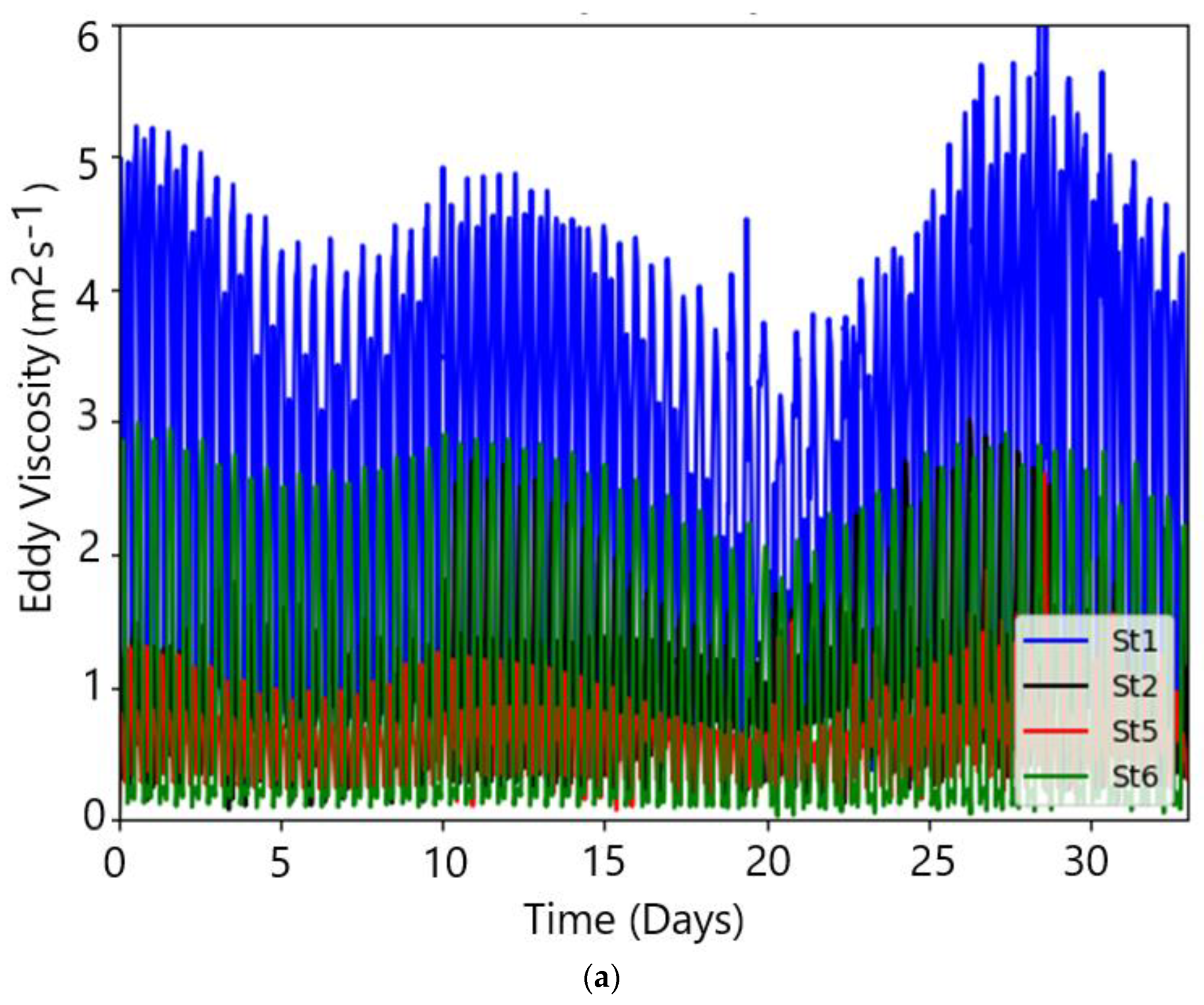
Figure 2 presents the simulated monthly time series of the horizontal and vertical eddy viscosities. As expected, the temporal evolution of the horizontal eddy viscosity follows a tidal cycle, i.e., a semidiurnal periodicity with a strong fortnightly modulation. The simulated values range within (0–6) m2/s are observed for St1, near the lagoon mouth. The maximum values are about twice as much as the ones observed for the innermost stations, St2, St5, and ST6. The vertical eddy viscosity is significantly lower than the horizontal eddy viscosity, the last ranging within (0, 25) 10−3 m2/s.
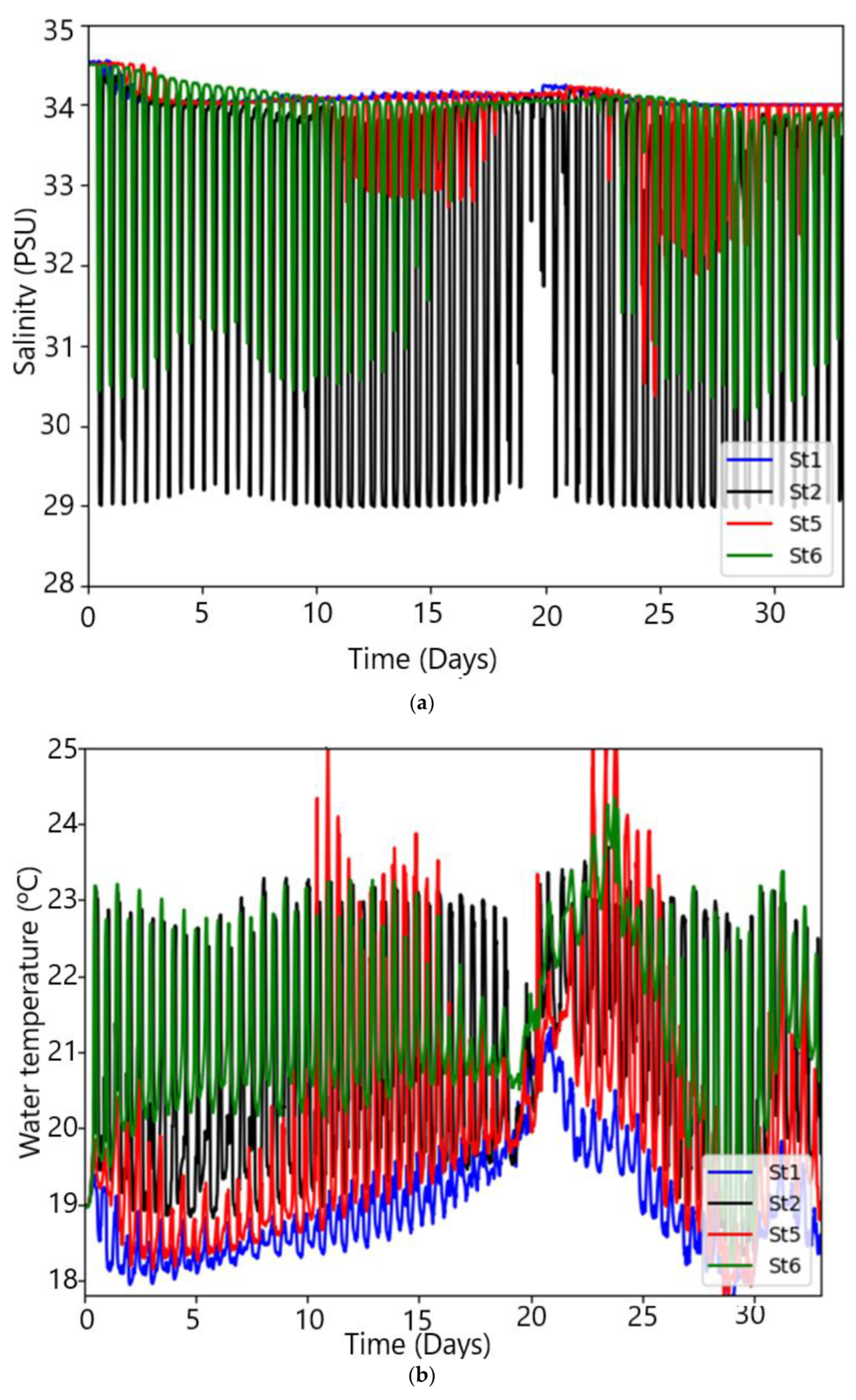
Figure 3a and Figure 3b present, respectively, the monthly time series for the salinity and temperature for June 2001.The salinity presents values close to the ocean ones, ~34 PSU, reflecting the low river flow regime and the tidal domination. The semi-diurnal oscillation is mostly evident for St2, which shows significant amplitude oscillation, ranging within (29–34) PSU, between the peak and trough. The fortnightly oscillations are mostly evident for St1, St5, and ST6, with amplitude oscillation ranging within (32–34) PSU. The water temperature (Figure 3b) shows a wide range of variation, within (18, 25) °C, depicting the diurnal influence of the radiative and the heat exchanges with the atmosphere, and the influence of the oceanic cold waters. Indeed, St1, despite the increasing water temperature trend during the first 15 days of June (18, 21) °C, cools down quickly to 18 °C due to the ocean cold water inflow. In contrast, the inner and shallow stations, St2 and St6, depict significant diurnal and semi-diurnal oscillations within the range (18, 23) °C, reflecting the competition between the diurnal warming and the ocean influence. St5, located in the main channel, has a similar trend as St2, additionally depicting the highest temperature values, ~25 °C, among the stations.
Figure 4a and Figure 4b present, respectively, the March 2001 monthly time series for the salinity and temperature. The salinity shows significant diurnal and fortnight amplitude oscillation, depicting a departure from the typical situation. When compared to June 2001, it can be observed that the salinity reflects the competition between the tides and the river forcing. Indeed, it shows a wide range of variation between peak and trough, within (20, 30) PSU, (0, 20) PSU, and (20, 25) PSU, for, respectively, St1, St2, and St5. Furthermore, the lower range of salinity values for St1 depicts an abnormal situation for the salinity when compared to the typical values within (30, 35) PSU. The salinity values for St2 and St5 attest to the abnormal transport of fresh and brackish water from the far ends and river mouths, which compete with the seawater flowing through the main channels. Finally, St6 shows almost low salinity values (<5 PSU), reflecting freshwater dominance. The simulated water temperature for March 2001 (Figure 4b) shows typical values for the season, as observed in Table 1. It presents a lower range of amplitude oscillation, from the trough values (~14 °C) to peak values up to 15.5 °C, reflecting the diurnal variation of the solar heating and the ocean tidal flow.

4.1.2. The k-ε/Sma Validation for the Salinity and Temperature

Dias et al. [80,81] previously implemented and assessed the hydrodynamic, salt, and heat transport models for the lagoon (the validation process included 11 stations) and showed that they could accurately simulate the salinity and the water temperature with significant accuracies (error: RMSE < 10%). Knowing that the selected four stations represent the main lagoon areas, the turbulence model validations are restricted to them without losing any generality concerning the other stations.
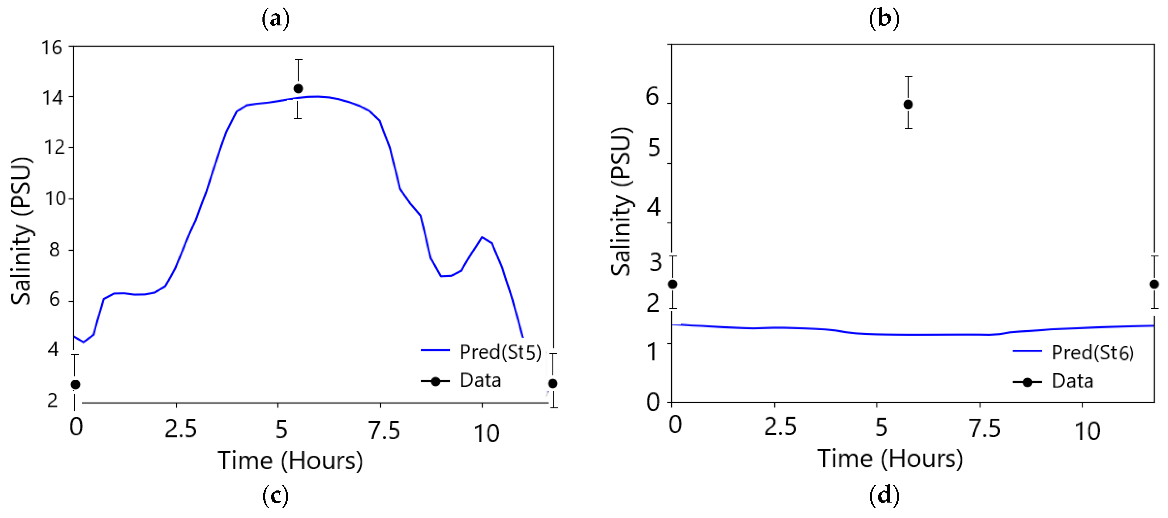
Figure 5 presents model results and data for one-half of the tidal cycle, for the salinity, for the selected stations. A good agreement can be observed between the model predictions and data. Nevertheless, the prediction for St6 (Figure 5d) is not quite as good as for St6: it strongly underestimates the maximum salinity value reached during the high tide (1,5 PSU to 6 PSU). This discrepancy may have to do with some model boundary adjustments to the river salinity, imposed to 0 PSU.
Figure 6 presents model results for the temperature for similar conditions as Figure 5. The agreement appears to be less good due to scale resolution, but the temperature range for both data and simulation is constrained within (13, 16) °C. The simulation underestimates the maximum temperature value for St6 by nearly 1 °C.
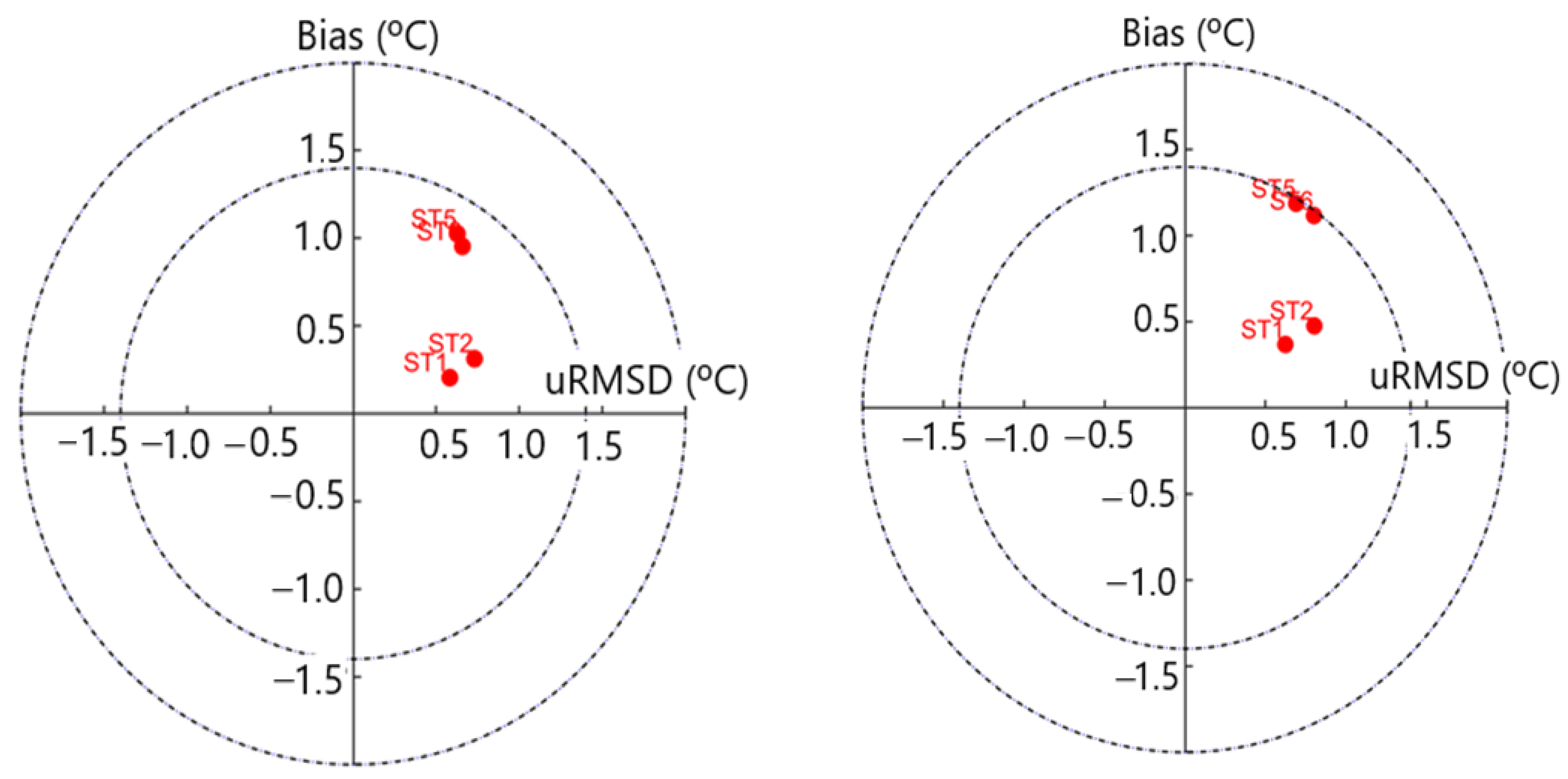
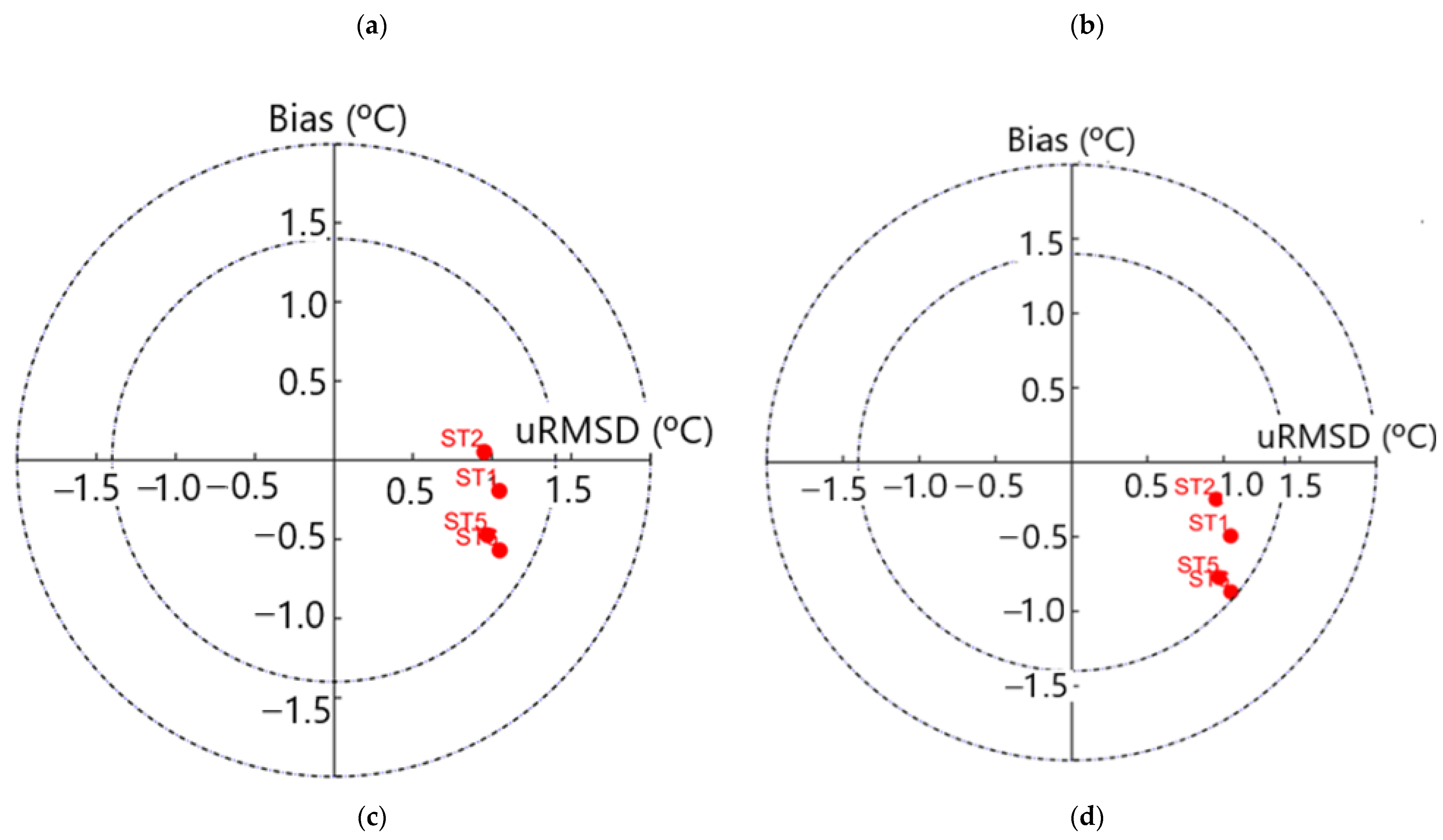
An objective evaluation of the model skill predictivity relative to data can be achieved through the target diagrams for salinity (Figure 7a–d) and temperature (Figure 8a–d), where a, b, c, and d correspond, respectively, to St1, St2, St5, and St6. Although each diagram refers to one station, the presence of the three other stations in the same figure has the purpose of assessing the salinity or temperature gradients between the stations. For instance, the diagram of Figure 6a gives the prediction for salinity for St1, while allowing us to assess the salinity departure from St2, St5, and St6. The x-axis and the y-axis indicate, respectively, the bias and the error of the model performance. Therefore, the bias provides an estimation of the deviation between predictions and data, whereas uRMSD is the respective error. The sign of the bias indicates if the model underestimates or overestimates data.
The diagrams for the salinity confirm that the model prediction for St1, St5, and St6, can be considered satisfactory. Indeed, the dots in Figure 7a–d, for, respectively, St1, St2, St5, and St6, are situated very close to the axis origins, corresponding to low values of the bias: the absolute values of the bias are of the order or smaller than 5 PSU, which indicates a small deviation of the simulations relative to the data. In all cases, the uRMSDs are below 5 PSU, corresponding to a relatively small error in the salinity assessment. In addition, it can be observed that St1 is ‘separated ‘ in salinity from the remaining stations by values greater than 10 PSU (up to 15 PSU for St6), while St5 and St6 are ‘very close’ from each other, reflecting the salinity gradients between the lagoon boundaries.
Likewise, the diagrams for the temperature reveal that the model prediction can be considered satisfactory. St1 presents, among the stations, the smallest bias values (~0.2 °C compared to ~0.5 °C), whereas St5 and St6 (Figure 8a,b) present the highest ones (~1.0 °C), confirming a worse prediction. On the other hand, the ‘geometrical distances’ in temperature between the stations depict the proximity of St1 and St2 and of St5 and St5 in term of temperature. This allows for estimating the horizontal temperature gradients between the areas close to the lagoon mouth (St1) and the inner areas (St5 and St6).

4.2. The Sensitivity Analysis of the Turbulence Models

A sensitivity analysis based on the statistical tools presented in Section 3.2.2 will be applied to the five turbulence models/schemes defined in Section 3.1.2. The cases M4 and M5, although unrealistic (considering the eddy viscosity constant), are helpful for the discussion.
The following variables were considered: the horizontal eddy viscosity, hereafter named eddy viscosity ( ν T H ), the salinity, and the temperature. As defined in the previous section, the ‘mvd’ and the ‘cdf’ sensitivity indexes are used to create diagrams that provide visual assessment of whether a specific parameter or model is sensitive concerning the baseline, in addition to allowing an estimation of the bias, as defined by RMSE (25). A ‘mvd’ equal to 0 implies that the ‘cdfs’ are similar, suggesting the insensitivity of a parameter or model. However, if it is equal to 1, the ‘cdfs’ are mutually exclusive, making the parameter or model extremely sensitive.
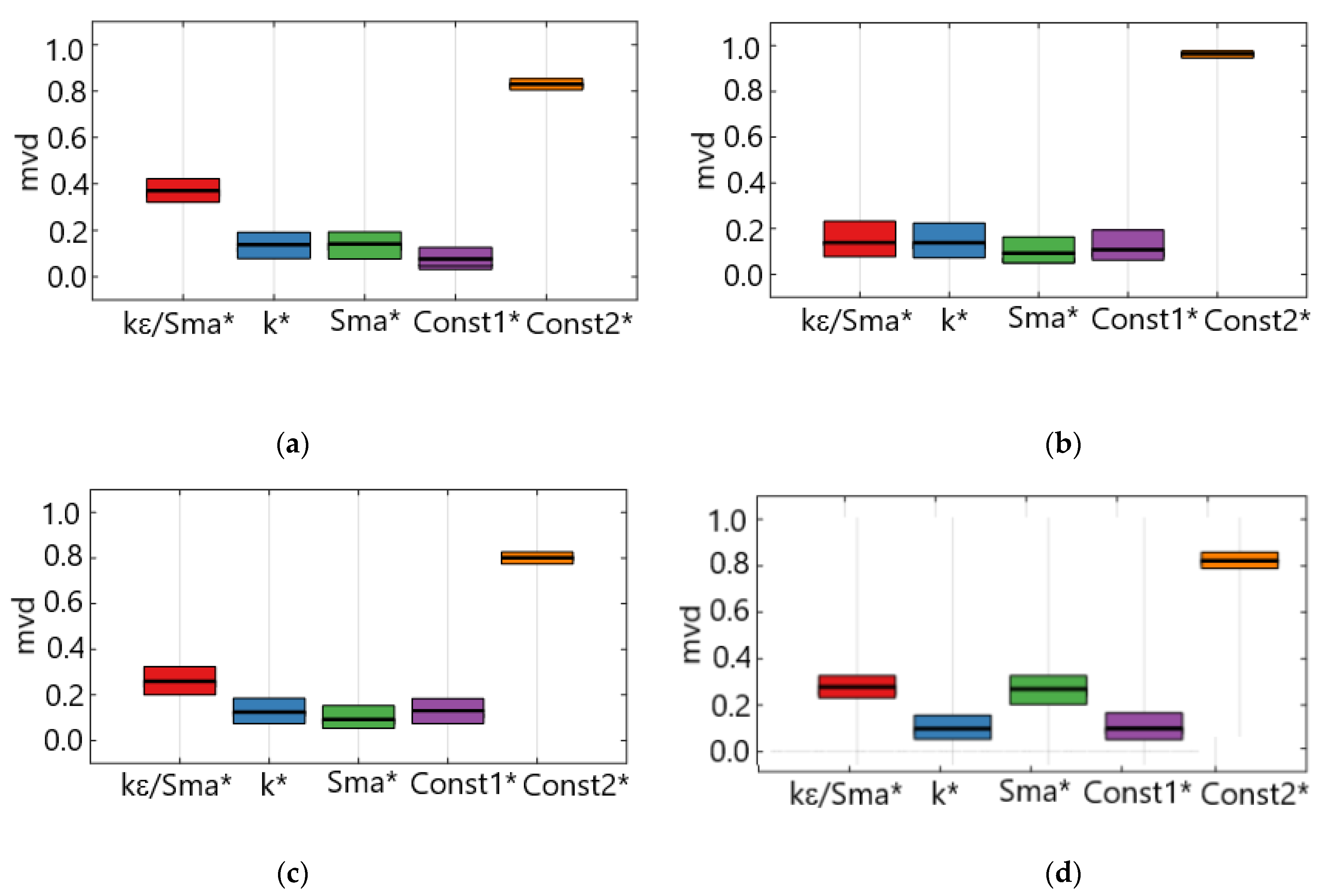
Figure 9a–d show the mvd indexes for the ν T H , for St1, St2, St5, and St6. k-ε*, k-ε/Sma*, k*, Sma*, Const1* and Const2* refer to non-dimensional ν T H calculated with k-ε, k-ε/Sma, k, Sma, Const1 and Const2, respectively, each one varying within (0, 1). It can be observed that M5 (( ν T H ), =10.0 m/s2) is the most responsive scheme, presenting the highest index value (~1.0), followed by M1 (k-ε/Sma) with a moderate value (~0.4), whereas the remaining schemes show lower index values (~0.1). In other words, M5 is the most sensitive, or M5 (( ν T H ), =10.0 m/s2) and M0 (k-ε) are mutually exclusive (or significantly different), whereas M2, M3, and M4 are quite insensitive. This result suggests that ν T H should be significantly lower than 10.0 m/s2 or the value is significantly different from the values calculated by M0. Using the same reasoning, the ν T H values calculated by M1 should be higher than those calculated by M2, M3, and M4. Figure 10 shows the cdf distribution for the eddy viscosity, restricted to St1 alone because St2, St5, and ST6 give similar results and are, therefore, omitted. It can be observed that M5 (( ν T H ), =10.0 m/s2) shows a significant cdf dispersion or a wide distribution (the lines representing the cdf’s) less tight for M1, and a very tight distribution for the remaining schemes, which is in line with the above conclusions concerning mvd. The above results allow estimating the value of ν T H , pointing out to be in the range (10−3, 5) m/s2, (see Figure 2a). Indeed, it was previously found that ν T H ranged within (0, 6) m2/s, where the maximum values were observed for St1. This comforts the choice of M1 as the favourite turbulence scheme. In addition, the cdf’s (Figure 10) provides an estimation of the RMSE, which corresponds to the bias between the schemes and the reference, as shown in the colour bar of the figure.
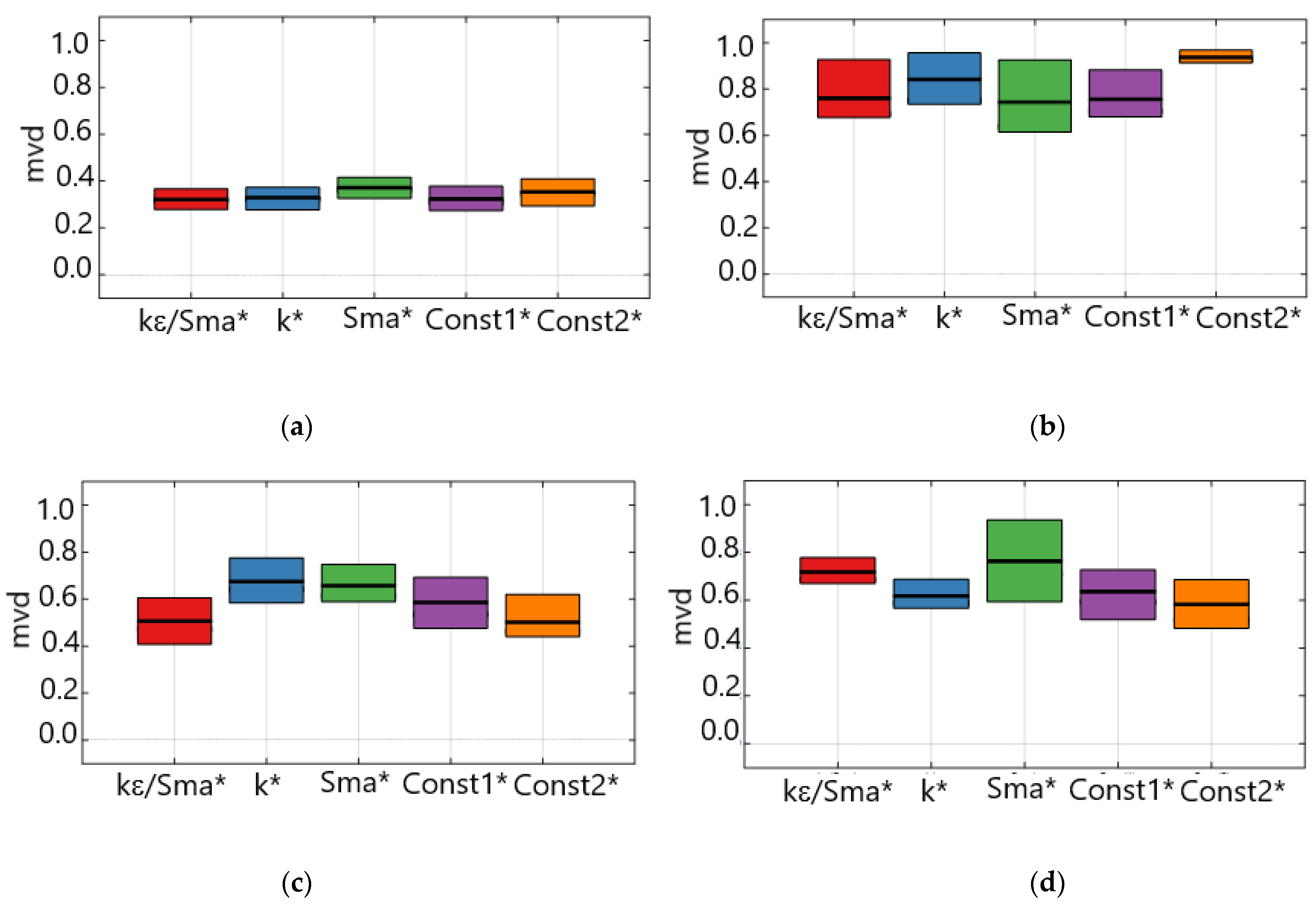
Figure 11a–d shows the mvd index for the salinity for the same stations as previously. St1 shows a low value of the index (<0.4) for all schemes, depicting low sensitivity, while St2, St5, and St6 show high values (>0.4). St2 shows index values of the order or higher than 0.8, with M5 presenting the highest values (~1). In other words, St2, St5, and St6 are more sensitive than S1 for the salinity relative to the baseline, suggesting that these stations exhibit significant salinity variability.
Figure 12a–d shows the mvd index for the temperature for the same stations as previously. St1 and St2 display moderate to high index values within the range (0.4, 0.6) for all schemes, whereas St5 and St6 show significantly higher values (0.4, 1.0), with st6 showing index values close to 1. In other words, St5 and St6 are the most sensitive stations to the temperature compared to the baseline or subjected to significant temperature variability. The distinction between the near-mouth deeper areas and the far-end shallow areas can account for this.

4.3. Taylor Diagrams for Predictive Skill of the Turbulence Models/Schemes

For better quantification of the RMSE, Taylor diagrams similar to Figure 8 were constructed (but not plotted) to obtain the bias and the error, uRMSD, associated with the turbulence models/schemes relatively to M0 (k-ε), as the last one was found to have, among the schemes, the lowest eddy viscosity values. Table 4 collects the bias (δ) for   v T H , the salinity, and the temperature (represented by, respectively, δ v H ,   δ S ,   and   δ T ).
Regarding   v T H , it can be observed that M5 and M2 present, respectively, the highest and the lowest bias values, respectively ~9.5 m2 s−1 and ~0 m2 s−1, whereas M1, M3, and M4 show moderate values (~1 m2 s−1). It is worth noting that St1 exhibits a high bias value, ~3 m2 s−1. uRMSD was typically low (<1 m2 s−1), except for 1.5 m2 s−1 for St1 for M1. This result confirms that v T H should be significantly lower than 10.0 m/s2 throughout the computational domain. Additionally, it indicates values that are significantly closer to the range (1, 3 m/s2), the last value being most probably observed for St1. The salinity presents, respectively, the smallest and the highest bias values, 0.1 PSU (uRMSD < 0.1 PSU) and 5-8 PSU (uRMSD ~ 10 PSU) for St1 and St2, respectively, while St5 and St6 exhibit intermediate bias value (<2.5 PSU (uRMSD < 5 PSU)). M2 consistently exhibits the lowest bias (~0), while M1, M3 M4, and M5 tend to present high values, >1 PSU. The result leads to the conclusion that the salinity variability was, respectively, the smallest for St1, the highest for St2, and moderate for the other stations. This can be explained by the competition between the ocean and the brackish water under typical wet conditions near St2 while still effective for the remaining stations. The temperature presented small bias values (<0.5 °C), except for the 1 °C for M3, for St2. It is worth noting that M5 presents the highest bias value, ~ 0.5 °C, except for the small value for St2 (~0.1 °C), and 1 °C for M3, for St2. The uRMSDs were low (<0.5 °C) across the stations and the schemes, except for ~1.0 °C for M3, M4, and M5, for St2. The findings imply that in contrast to the salinity, the water temperature variability throughout the main lagoon stations is moderate.

4.4. The Sensitivity Analysis of the k-ε/Sma Turbulence Parameters

The main parameters entering the turbulence models are often considered ’universal’, so their values are not generally changed. It leaves Cμ, Csm, σε, σk, and σT as the free parameters for k-ε/Sma. Therefore, a sensitivity analysis was performed to identify each parameter’s influence on the simulation outputs. The sensitivity of the selected constant was examined for up to ±100% adjustment of their values, tested individually, relative to the reference values presented in Section 3.1.2. A high river flow input (similar to March 2001; see Table 2) was used for June 2001 simulations to produce high salinity and temperature gradient effects between the lagoon margins to enhance the eddy diffusivity effect on salinity and temperature.
The main results are summarised in Table 5. The eddy viscosity coefficient shows significant sensitivity to the parameters. The lower and upper limits of the parameters resulted in variation (RMSE) within the range (1, 4) m2 s−1, which is up to 100% of the typical values for the baseline situation. It is worth noting that St1 shows the most significant variation of the coefficient (~4 m2 s−1). The water temperature shows moderate sensitivity to the parameters. Lower and upper limits of the parameters resulted in changes of the order of 2.20 °C, which is up to 10% changes from the typical temperature values for the baseline situation. The salinity variation ranges evidence significant sensitivity to the parameters. The lower and upper limits lower of the parameters resulted in deviations within the range (0, 13) PSU, or nearly 100% of the typical salinity values from the baseline situation. It is worth noting again that St1 shows the most significant salinity variation (~13 PSU).

5. Discussion and Concluding Remarks

The best turbulence model is essential for the stability conditions of the hydrodynamic and transport models, and better simulates the transport of dissolved or suspended substances. Indeed, horizontal transport is significantly impacted by turbulence in shallow water systems.
The main goal of this study was to assess the performance of four turbulence schemes/models (k, k-ε, Smagorinsky’s turbulence model, and k-ε/Smagorinsky’s). For this purpose, they were used to simulate the eddy viscosity, the salinity, and the temperature inside the Ria de Aveiro lagoon.
The statistical tools were also used to objectively evaluate the relative skill of the model’s predictivity. Both direct comparison and target diagrams for salinity and temperature reveal that the model prediction can be considered satisfactory. The model can be regarded as an operative tool to correctly simulate transport of dissolved or suspended substances. The k-ε/Smagorinsky’s model/scheme offered more accurate estimates of the eddy viscosity when compared to the other models/schemes. Furthermore, the scheme supports mixing fluid flows of variable density; therefore, it should better simulate the lagoon’s variability and the response to any dynamic changes inside the water body. Indeed, it was found that the eddy viscosity ranged within (1, 6) m2 s−1, most probably within (1–3) m2 s−1. More specifically, St1 had an estimated top value close to 3 m2 s−1, whereas inner areas showed more moderate values (~1 m2 s−1). Indeed, St1 is situated close to the lagoon mouth, at the ocean border, where the water flow is the most intense (the current intensity reaches peak values close to 1.5 m s−1 [27,28,29]). Applying the sensitivity analysis to the salinity showed that St1 presented the lowest sensitivity index relative to the baseline. At the same time, St2, St5, and St6 had the highest values; among them, St2 showed the highest one, although more moderate for the other station. This outcome is consistent with that the most significant salinity variations occur mid-distance between the oceanic and riverine boundaries. In contrast, St5 and St6 appear to be the most sensitive to temperature, reflecting the most susceptible areas to water temperature variations and competition between cold oceanic and warmer inland waters. In addition, it was able to have a picture of the salinity and the temperature gradients inside the lagoon for the condition of the experiments. In the case of the extremely wet situation, a high salinity ‘gradient’, in the range (10, 20) PSU, was set up between the mouth and the far end areas. The temperature shows moderate ‘gradients’, of the order or below 1 °C. In addition, each couple of stations (St1 and St2, or St5 and St6) show similar temperature values (differences between temperature stations of approximately 0.5 °C). In contrast, between the two couples of stations, the difference is of the order of 1 °C, reflecting the water’s inertia to the heat exchanges, the influence of the tidal dynamics, and the influence of the distance from the lagoon mouth and the far ends. Overall, the results evidenced that k-ε/Smagorinsky’s outperforms the competing schemes supporting the choice as the reference scheme. The application of the sensitivity analysis to the non-universal parameters of the k-ε/Smagorinsky schemes (Cm, Csm, σε), relative to the reference values, for up to ±100% adjustment of their values, evidenced significant sensitivity for the eddy viscosity and the salinity. The induced changes fall within the range (1, 4) m2 s−1 and (0, 13) PSU, respectively, representing up to 100% of the typical values for the baseline situation. In particular, the areas close to the lagoon mouth evidenced the most significant variation of the eddy viscosity coefficient (~4 m2 s−1) and the salinity (~13 PSU). The water temperature evidenced moderate sensitivity to the parameters, with a variation within the range of (1, 2.20) °C, up to a 10% deviation from the typical temperature values for the baseline situation. Despite the moderate variation, this value is significant, considering the water inertia to the temperature changes.

Funding

This work is a contribution to project ASHMOB (PTDC/ASP-SIL/29351/2017) funded by FCT—Fundação para a Ciência e a Tecnologia, I.P., through national funds, and the co-funding by the FEDER, within the PT2020 Partnership Agreement and Compete 2020. Thanks are due to FCT/MCTES for the financial support to CESAM.

Institutional Review Board Statement

Not applicable.

Informed Consent Statement

Not applicable.

Data Availability Statement

Data used in this study is not available in a publicly accessible repository. References to this data can be found here: Modelria Project reports FCT—ModelRia (POCTI/MGS/10219/1998), which is linked to https://ria.ua.pt/handle/10773/11275?mode=full (accessed on 1 September 2022) and http://hdl.handle.net/10773/11275 (accessed on 1 September 2022).

Acknowledgments

The author is indebted to the communities behind the open-source software packages SAFE and the Skill Metrics Toolbox.

Conflicts of Interest

The author declares no conflict of interest.

Nomenclature

SmaSmagorinsky

References

  1. Hall, P.; Ozcakir, O. Poiseuille flow in rough pipes: Linear instability induced by vortex-wave interactions. J. Fluid Mech. 2021, 913, A43. [Google Scholar] [CrossRef]
  2. Lauga, E.; Powers, T.R. The hydrodynamics of swimming microorganisms. Rep. Prog. Phys. 2009, 72, 096601. [Google Scholar] [CrossRef]
  3. Lopez-Santana, G.; Kennaugh, A.; Keshmiri, A. Experimental Techniques against RANS Method in a Fully Developed Turbulent Pipe Flow: Evolution of Experimental and Computational Methods for the Study of Turbulence. Fluids 2022, 7, 78. [Google Scholar] [CrossRef]
  4. Hongyou, L.; Yanxiong, S.; Xiaojing, Z. Evolution of turbulent kinetic energy during the entire sandstorm process. Atmos. Chem. Phys. 2022, 22, 8787–8803. [Google Scholar] [CrossRef]
  5. Akira, N.; Takuya, H.; Keisuke, A.; Hiroyuki, M. Interannual Bottom-Intensified Current Thickening Observed on the Continental Slope off the Southeastern Coast of Hokkaido, Japan. Fluids 2022, 7, 84. [Google Scholar] [CrossRef]
  6. Fox-Kemper, B.; Adcroft, A.; Böning, C.W.; Chassignet, E.P.; Curchitser, E.; Danabasoglu, G.; Eden, C.; England, M.H.; Gerdes, R.; Greatbatch, R.J.; et al. Challenges and prospects in ocean circulation models. Front. Mar. Sci. 2019, 6, 65. [Google Scholar] [CrossRef] [Green Version]
  7. Aluie, H. Coarse-grained incompressible magnetohydrodynamics: Analyzing the turbulent cascades. New J. Phys. 2017, 19, 025008. [Google Scholar] [CrossRef]
  8. Zweibel, E.G. The basis for cosmic ray feedback: Written on the wind. Phys. Plasmas 2017, 24, 055402. [Google Scholar] [CrossRef] [Green Version]
  9. Bang, C.S.; Rana, Z.A.; Könözsy, L.; Marchante, R.V.; Temple, C. Numerical Investigation and Fluid-Structure Interaction (FSI) Analysis on a Double-Element Simplified Formula One (F1) Composite Wing in the Presence of Ground Effect. Fluids 2022, 7, 85. [Google Scholar] [CrossRef]
  10. Kajiwara, S. Improvement of Gas–Liquid Separation Performance of Engine Oil Using Swirling. Fluids 2022, 7, 304. [Google Scholar] [CrossRef]
  11. Abramov, R.V. Creation of turbulence in polyatomic gas flow via an intermolecular potential. Phys. Rev. Fluids 2022, 7, 054605. [Google Scholar] [CrossRef]
  12. Islam, H.; Sutulo, S.; Soares, C.G. Aerodynamic Load Prediction on a Patrol Vessel Using Computational Fluid Dynamics. J. Mar. Sci. Eng. 2022, 10, 935. [Google Scholar] [CrossRef]
  13. Lee, T.W.; Park, J.E. Entropy and Turbulence Structure. Entropy 2022, 24, 11. [Google Scholar] [CrossRef] [PubMed]
  14. Prandtl, L. 7. Bericht über Untersuchungen zur ausgebildeten Turbulenz. ZAMM-J. Appl. Math. Mech./Z. Angew. Math. Mech. 1925, 5, 136–139. [Google Scholar]
  15. Rousseau, G.; Ancey, C. An experimental investigation of turbulent free-surface flows over a steep permeable bed. J. Fluid Mech. 2022, 941, A51. [Google Scholar] [CrossRef]
  16. Smagorinsky, J. General circulation experiments with the primitive equations. I. the basic experiment. Mon. Weather Rev. 1963, 91, 99–164. [Google Scholar] [CrossRef]
  17. Smagorinsky, J. Some historical remarks on the use of nonlinear viscosities. In Large Eddy Simulation of Complex Engineering and Geophysical Flows; Cambridge University Press: New York, NY, USA, 1993; pp. 3–36. [Google Scholar]
  18. Meneveau, C. Turbulence: Subgrid-Scale Modeling. Scholarpedia 2010, 5, 9489. [Google Scholar] [CrossRef]
  19. Burman, E.; Hansbo, P.; Larson, M.G. Error Estimates for the Smagorinsky Turbulence Model: Enhanced Stability through Scale Separation and Numerical Stabilization. J. Math. Fluid Mech. 2022, 24, 5. [Google Scholar] [CrossRef]
  20. Cushman-Roisin, B.; Gualtieri, C.; Mihailovic, D. Environmental Fluid Mechanics: Current issues and future outlook. In Fluid Mechanics of Environmental Interfaces, 2nd ed.; Gualtieri, C., Mihailovic, D., Eds.; CRC Press/Balkema: Boca Raton, FA, USA, 2012; pp. 3–17. [Google Scholar]
  21. Dauxois, T.; Peacock, T.; Bauer, P.; Caulfield, C.P.; Cenedese, C.; Gorlé, C.; Haller, G.; Ivey, G.N.; Linden, P.F.; Meiburg, E.; et al. Confronting Grand Challenges in environmental fluid mechanics. Phys Rev. Fluids 2021, 6, 020501. [Google Scholar] [CrossRef]
  22. Alfonsi, G. Reynolds-Averaged Navier-Stokes Equations for Turbulence Modeling. Appl. Mech. Rev. 2009, 62, 040802. [Google Scholar] [CrossRef]
  23. Siti, S.N.A.; Asako, Y.; Sidik, N.A.C.; Mohamed, S.B.; Japar, W.M.A.A. A short review on RANS turbulence models. CFD Lett. 2020, 12, 83–96. [Google Scholar]
  24. Li, Y.; Jiakuan, X.; Qiao, L.; Zhang, Y.; Junqiang, B. A novel local-variable-based Reynolds-averaged Navier–Stokes closure model for bypass and laminar separation induced transition. Phys. Fluids 2021, 33, 104103. [Google Scholar] [CrossRef]
  25. Na, J.S.; Taekyun, K.; Kyung, J.E.; Seung-Tae, Y.; Won Sang, L.; Sukyoung, Y.; Jiyeon, L. Large-eddy simulations of the ice-shelf–ocean boundary layer near the ice front of Nansen Ice Shelf, Antarctica. Cryosphere 2022, 16, 3451–3468. [Google Scholar] [CrossRef]
  26. Gayen, B.; Griffiths, R.W.; Kerr, R.C. Simulation of convection at a vertical ice face dissolving into saline water. J. Fluid Mech. 2016, 798, 284–298. [Google Scholar] [CrossRef]
  27. Mondal, M.; Gayen, B.; Kerr, R. Ablation of sloping ice faces into polar seawater. J. Fluid Mech. 2019, 863, 545–571. [Google Scholar] [CrossRef] [Green Version]
  28. Vreugdenhil, C.A.; Taylor, J.R. Stratification effects in the turbulent boundary layer beneath a melting ice shelf: Insights from resolved large-eddy simulations. J. Phys. Oceanogr. 2019, 49, 1905–1925. [Google Scholar] [CrossRef] [Green Version]
  29. Sridhar, A.; Tissaoui, Y.; Marras, S.; Shen, Z.; Kawczynski, C.; Byrne, S.; Pamnany, K.; Waruszewski, M.; Gibson, T.; Kozdon, J.; et al. Large-eddy simulations with climatemachine v0. 2.0: A new open-source code for atmospheric simulations on gpus and cpus. Geosci. Model Dev. 2022, 15, 6259–6284. [Google Scholar] [CrossRef]
  30. Deskos, G.; Lee, J.C.Y.; Draxl, C.; Sprague, M.A. Review of Wind–Wave Coupling Models for Large-Eddy Simulation of the Marine Atmospheric Boundary Layer. J. Atmos. Sci. 2021, 78, 3025–3046. [Google Scholar] [CrossRef]
  31. Xu, C.Y.; Sun, Z.; Zhang, Y.T.; Sun, J.H. Improvement of the scale-adaptive simulation technique based on a compensated strategy. Eur. J. Mech.-B/Fluids 2020, 81, 1–14. [Google Scholar] [CrossRef]
  32. Menter, F.R.; Egorov, Y. The scale-adaptive simulation method for unsteady turbulent flow predictions. Part 2: Application to complex flows. Flow Turbul. Combust. 2010, 85, 139–165. [Google Scholar] [CrossRef]
  33. Xu, C.Y.; Zhou, T.; Wang, C.L.; Sun, J.H. Applications of scale-adaptive simulation technique based on one-equation turbulence model. Appl. Math. Mech.-Engl. Ed. 2015, 36, 121–130. [Google Scholar] [CrossRef]
  34. Launder, B.E. Advanced Turbulence Models for Industrial Applications. In Turbulence and Transition Modelling; Hallbäck, M., Henningson, D.S., Johansson, A.V., Alfredsson, P.H., Eds.; ERCOFTAC Series; Springer: Dordrecht, The Netherlands, 1996; Volume 2. [Google Scholar] [CrossRef]
  35. Launder, B.E.; Spalding, D.B. Mathematical Models of Turbulence; Academic Press: London, UK, 1972. [Google Scholar]
  36. Launder, B.E.; Spalding, D.B. Turbulence models and their application to the prediction of internal flows. Heat Fluid Flow 1972, 2, 43–54. [Google Scholar]
  37. Harlow, F.H. (Ed.) Turbulence Transport Modelling; AIAA: New York, NY, USA, 1973. [Google Scholar]
  38. Mellor, G.L. Analytic Prediction of the Properties of Stratified Planetary Surface Layers. J. Atmos. Sci. 1973, 30, 1061–1069. [Google Scholar] [CrossRef]
  39. Mellor, G.L.; Yamada, T. A Hierarchy of Turbulence Closure Models for Planetary Boundary Layers. J. Atmos. Sci. 1974, 31, 1791–1806. [Google Scholar] [CrossRef]
  40. Mellor, G.L.; Yamada, T. Development of a Turbulence Closure Model for Geophysical Fluid Problems. Rev. Geophys. Space Phys. 1982, 20, 851–875. [Google Scholar] [CrossRef] [Green Version]
  41. Mellor, G.; Herring, H.J. A survey of the mean turbulent field closure models. AIAA J. 1973, 11, 590. [Google Scholar] [CrossRef]
  42. Burchard, H. Applied turbulence modelling in marine waters. In Lecture Notes in Earth Sciences; Springer: Berlin/Heidelberg, Germany, 2000; Volume 100, p. 229. [Google Scholar]
  43. Burchard, H.; Gräwe, U.; Peter, H.; Klingbeil, K.; Umlauf, L. Turbulence Closure Modelling in Coastal Waters. Die Küste 2014, 81, 69–87. [Google Scholar]
  44. Burchard, H.; Petersen, O.; Rippeth, T.P. Comparing the performance of the Mellor-Yamada and the k-ε two-equation turbulence models. J. Geophys. Res. 1998, 103, 10543–10554. [Google Scholar] [CrossRef] [Green Version]
  45. Burchard, H.; Baumert, H. On the performance of a mixed-layer model based on the k-ε turbulence closure. J. Geophys. Res. 1995, 100, 8523–8540. [Google Scholar] [CrossRef]
  46. Burchard, H.; Bolding, K. Comparative Analysis of Four Second-Moment Turbulence Closure Models for the Oceanic Mixed Layer. J. Geophys. Res. 2001, 31, 1943–1968. [Google Scholar] [CrossRef]
  47. Hami, K. Turbulence Modeling a Review for Different Used Methods. Int. J. Heat Technol. 2021, 39, 227–234. [Google Scholar] [CrossRef]
  48. Zeng, X.P.; Wang, Y.S.; MacCall, B.T. A k-ε turbulence model for the stable atmosphere. J. Atmos. Sci. 2019, 77, 167–184. [Google Scholar] [CrossRef]
  49. Zhao, M.; Wan, D.; Gao, Y. Comparative Study of Different Turbulence Models for Cavitational Flows around NACA0012 Hydrofoil. J. Mar. Sci. Eng. 2021, 9, 742. [Google Scholar] [CrossRef]
  50. MIKE 3 Hydrodynamic and Transport Module, A Scientific Description. DHI Water and Environment. Available online: https://manuals.mikepoweredbydhi.help/2017/Coast_and_Sea/MIKE_321_FM_Scientific_Doc.pdf (accessed on 1 September 2022).
  51. Moreira, M.H.; Queiroga, H.; Machado, M.M.; Cunha, M.R. Environmental gradients in a southern estuarine system: Ria de Aveiro, Portugal, implication for soft bottom macrofauna colonization. Aquatic Ecol. 1993, 27, 465–482. [Google Scholar] [CrossRef]
  52. Génio, L.; Sousa, A.; Vaz, N.; Dias, J.M.; Barroso, C. Effect of low salinity on the survival of recently hatched veliger of Nassarius reticulatus (L.) in estuarine habitats: A case study of Ria de Aveiro. J. Sea Res. 2008, 59, 133–143. [Google Scholar] [CrossRef]
  53. Vargas, C.I.C.; Vaz, N.; Dias, J.M. An evaluation of climate change effects in estuarine salinity patterns: Application to Ria de Aveiro shallow water system. Estuar. Coast. Shelf Sci. 2017, 189, 33–45. [Google Scholar] [CrossRef]
  54. Dias, J.M. Contribution to the Study of the Ria de Aveiro hydrodynamics. Ph.D. Thesis, Universidade de Aveiro, Aveiro, Portugal, 2001; p. 288. [Google Scholar]
  55. Dias, J.M.; Lopes, J.F.; Dekeyser, I. Hydrological characterisation of Ria de Aveiro lagoon, Portugal, in early summer. Oceanol. Acta 1999, 22, 473–485. [Google Scholar] [CrossRef] [Green Version]
  56. Vaz, N.; Dias, J.M. Hydrographic characterization of an estuarine tidal channel. J. Mar. Syst. 2008, 70, 168–181. [Google Scholar] [CrossRef]
  57. ModelRia. Modelação da qualidade da água na laguna da Ria de Aveiro; Final Report; Universidade de Aveiro-Centro das Zonas Costeiras e do Mar, Instituto Superior Técnico–Centro de Ambiente e Tecnologias Marítimos and Hidromod: Aveiro, Portugal, 2003. [Google Scholar]
  58. Rodrigues, M.; Oliveira, A.; Queiroga, H.; Fortunato, A.B.; Zhang, Y.J. Three-dimensional modeling of the lower trophic levels in the Ria de Aveiro (Portugal). Ecol. Model. 2009, 220, 1274–1290. [Google Scholar] [CrossRef]
  59. Almeida, M.A.; Cunha, M.A.; Alcântara, F. Relationship of bacterioplankton production with primary production and respiration in a shallow estuarine system, Ria de Aveiro, NW Portugal. Microbiol. Res. 2005, 160, 315–328. [Google Scholar] [CrossRef] [PubMed]
  60. Lopes, C.B.; Lillebo, A.I.; Dias, J.M.; Pereira, E.; Vale, C.; Duarte, A.C. Nutrient dynamics and seasonal succession of phytoplankton assemblages in a Southern European Estuary: Ria de Aveiro, Portugal. Estuar. Coast. Shelf Sci. 2007, 71, 480–490. [Google Scholar] [CrossRef]
  61. MIKE 3 Flow Model, Hydrodynamic Module, Scientific Documentation. DHI Water and Environment. Available online: https://manuals.mikepoweredbydhi.help/2019/Coast_and_Sea/m3HD.pdf (accessed on 1 September 2022).
  62. MIKE 21 & MIKE 3 Flow Model FM Hydrodynamic and Transport Module Scientific Documentation. DHI Water and Environment. Available online: https://manuals.mikepoweredbydhi.help/2017/Coast_and_Sea/MIKE_321_FM_Scientific_Doc.pdf (accessed on 1 September 2022).
  63. Jolliff, J.K.; Kindle, J.C.; Shulman, I.; Penta, B.; Friedrichs, M.; Helber, R.; Arnone, R. Skill Assessment for Coupled Biological/Physical Models of Marine Systems. J. Mar. Syst. 2009, 76, 64–82. [Google Scholar] [CrossRef]
  64. Rochford, P.A. Skill Metrics Toolbox. Retrieved from MathWorks File Exchange. 2020. Available online: https://www.mathworks.com/matlabcentral/fileexchange/52943-peterrochford-skillmetricstoolbox (accessed on 1 September 2022).
  65. Taylor, K.E. Summarizing multiple aspects of model performance in a single diagram. J. Geophys. Res. 2001, 106, 7183–7192. [Google Scholar] [CrossRef]
  66. Norton, J. An introduction to sensitivity assessment of simulation models. Environ. Model. Softw. 2015, 69, 166–174. [Google Scholar] [CrossRef]
  67. Pianosi, F.; Sarrazin, F.; Wagener, T. A matlab toolbox for global sensitivity analysis. Environ. Model. Softw. 2015, 70, 80–85. [Google Scholar] [CrossRef] [Green Version]
  68. Pianosi, F.; Wagener, T. A simple and efficient method for global sensitivity analysis based on cumulative distribution functions. Environ. Model. Softw. 2015, 67, 1–11. [Google Scholar] [CrossRef] [Green Version]
  69. Pianosi, F.; Wagener, T. Understanding the time-varying importance of different uncertainty sources in hydrological modelling using global sensitivity analysis. Hydrol. Process. 2016, 30, 3991–4003. [Google Scholar] [CrossRef] [Green Version]
  70. Young, P.C.; Spear, R.C.; Hornberger, G.M. Modeling badly defined systems: Some further thoughts. In Proceedings of the SIMSIG Conference, Canberra, Australia, 4–6 September 1978; pp. 24–32. [Google Scholar]
  71. Spear, R.; Hornberger, G. Eutrophication in peel inlet. II. Identification of critical uncertainties via generalized sensitivity analysis. Water Res. 1980, 14, 43–49. [Google Scholar] [CrossRef]
  72. Freer, J.; Beven, K.; Ambroise, B. Bayesian estimation of uncertainty in runoff prediction and the value of data: An application of the GLUE approach. Water Resour. Res. 1996, 32, 2161–2173. [Google Scholar] [CrossRef]
  73. Wagener, T.; Boyle, D.; Lees, M.; Wheater, H.; Gupta, H.; Sorooshian, S. A framework for development and application of hydrological models. Hydrol. Earth Syst. Sci. 2001, 5, 13–26. [Google Scholar] [CrossRef]
  74. Sieber, A.; Uhlenbrook, S. Sensitivity analyses of a distributed catchment model to verify the model structure. J. Hydrol. 2005, 310, 216–235. [Google Scholar] [CrossRef]
  75. Sarrazin, F.J.; Pianosi, F.; Wagener, T. Global Sensitivity Analysis of environmental models: Convergence and validation. Env. Model. Soft. 2016, 79, 135–152. [Google Scholar] [CrossRef] [Green Version]
  76. Sarrazin, F.; Pianosi, J.; Wagener, F. An Introduction to the SAFE Matlab Toolbox with Practical Examples and Guidelines; Petropoulos, G., Srivastava, P., Eds.; Elsevier Inc.: Amsterdam, The Netherlands, 2017; pp. 363–378. [Google Scholar]
  77. Kolmogorov, A.N. Foundations of Probability Theory; Julius Springer: Berlin, Germany, 1939. [Google Scholar]
  78. Smirnov, N. On the estimation of the discrepancy between empirical curves of distribution for two independent samples. Bull. Math. Univ. Mosc. 1939, 2, 3–14. [Google Scholar]
  79. Parra, V.; Fuentes-Aguilera, P.; Muñoz, E. Identifying advantages and drawbacks of two hydrological models based on a sensitivity analysis: A study in two Chilean watersheds. Hydrol. Sci. J. 2018, 63, 1831–1843. [Google Scholar] [CrossRef]
  80. Dias, J.M.; Lopes, J.F.; Dekeyser, I. A numerical system to study the transport properties in the Ria de Aveiro lagoon. Ocean Dyn. 2003, 53, 220–231. [Google Scholar] [CrossRef]
  81. Dias, J.M.; Lopes, J.F. Implementation and evaluation of hydrodynamic, salt and heat transport models: The case of Ria de Aveiro Lagoon, Portugal. Environ. Model. Softw. 2006, 21, 1–15. [Google Scholar] [CrossRef]
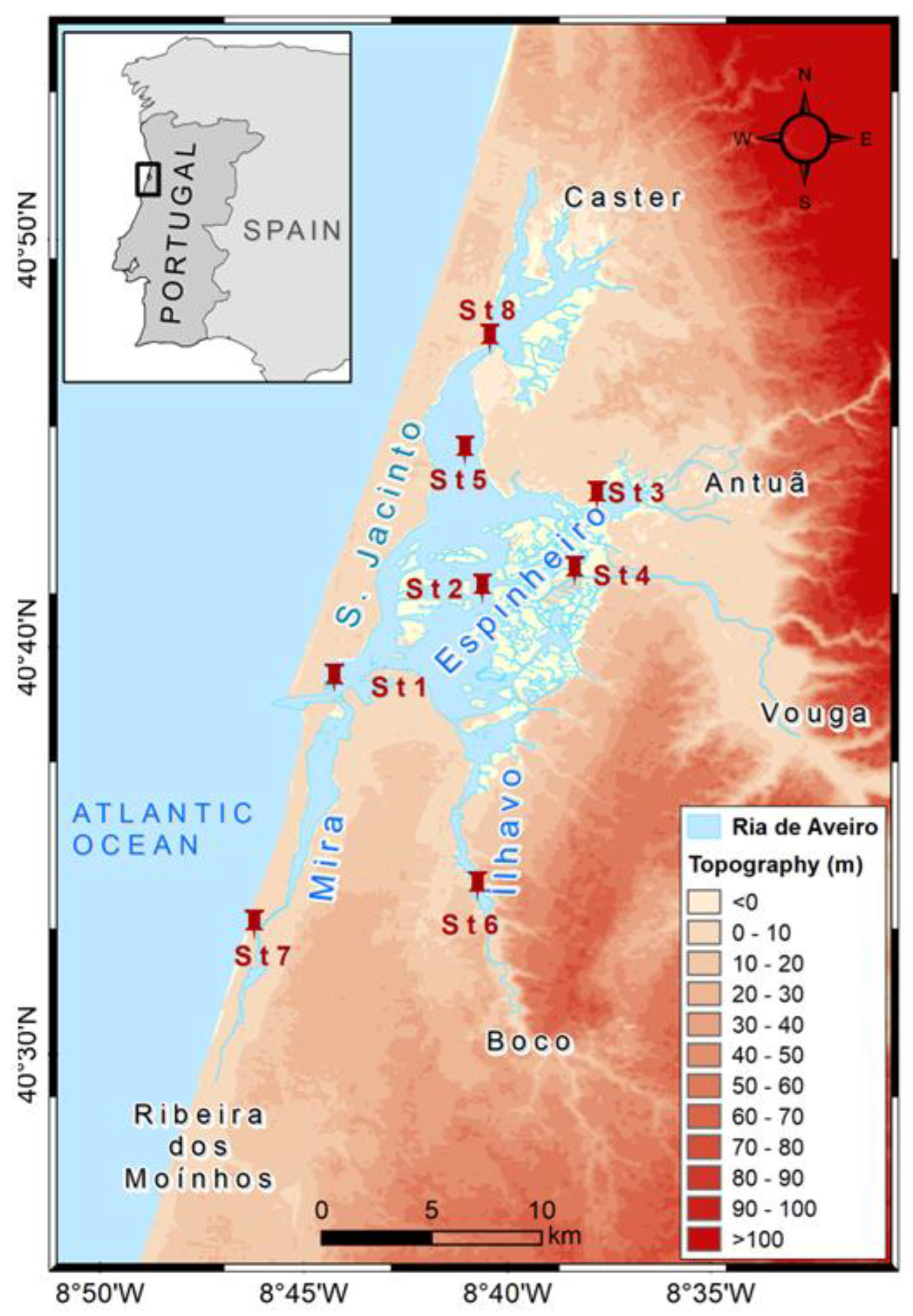
Figure 1. The study area: The Ria de Aveiro lagoon, with the location of the stations (St1St8).
Jmse 10 01750 g001
Figure 2. (a) Simulated horizontal eddy viscosity for St1, St2, St5, and St6. (b) Simulated vertical eddy viscosity for St1, St2, St5, and St6.
Jmse 10 01750 g002aJmse 10 01750 g002b
Figure 3. (a) Simulated salinity for June 2001, simulated for St1, St2, St3, and St4. (b) Simulated water temperature for June 2001, for St1, St2, St3, and St4.
Jmse 10 01750 g003
Figure 4. (a) Simulated salinity for March 2001, for St1, St2, St5, and St6. (b) Simulated water temperature for March 2001, for St1, St2, St5, and St6.
Jmse 10 01750 g004aJmse 10 01750 g004b
Figure 5. Simulation (line) and data (dot) for the salinity (a)—St1; (b)—St2(b); (c)—St5; (d)—St6.
Jmse 10 01750 g005aJmse 10 01750 g005b
Figure 6. Simulation (line) and data (dot) for the temperature (a)—St1; (b)—St2(b); (c)—St5; (d)—St6).
Jmse 10 01750 g006
Figure 7. Target diagrams for salinity for St1 (a), St2 (b), St5 (c), and St6 (d).
Jmse 10 01750 g007aJmse 10 01750 g007b
Figure 8. Target diagrams for temperature for St1 (a), St2 (b), St5 (c), and St6 (d).
Jmse 10 01750 g008aJmse 10 01750 g008b
Figure 9. Mvd (a) index for the eddy viscosity ( ν T ), for St1 (a), St2 (b) St4 (c) and St6 (d).
Jmse 10 01750 g009
Figure 10. Cdf for the eddy viscosity ( ν T ), for St1.
Jmse 10 01750 g010
Figure 11. Mvd index for the salinity, for St1 (a), St2 (b), St5 (c), and St6 (d).
Jmse 10 01750 g011
Figure 12. Mvd index for the temperature, for St1 (a), St2 (b), St5 (c), and St6 (d).
Jmse 10 01750 g012aJmse 10 01750 g012b
Table 1. Salinity and temperature for March (*) 2001 and for June (**) 2001, according to observations [57,58,59,60].
Stations Salinity *
(PSU)
Water Temp *
(°C)
Salinity **
(PSU)
Water Temp **
(°C)
St1Min.7.8 (ebb)13.232.518
Max.29 (flood)15.735.119.5
St2Min.0.1 (ebb)12.833.618
Max.4.8 (flood)14.034.420
St3Min.0.6 (ebb)13.832.721.5
Max.7 (flood)15.133.821.8
St4Min.0.016.830.019.4
Max.0.018.230.021.5
St5Min.8 (ebb)14.534.120.8
Max.22 (flood)16.034.722.0
St6Min.1.5 (ebb)14.832.520.0
Max.5.0 (flood)16.034.424.0
St7Min.1.0 (ebb)15.129.219.2
Max.7.0 (flood)16.030.220.5
St8Min.1.0 (ebb)15.229.220.5
Max.7.0 (flood)16.333.221.5
Table 2. Freshwater and ocean boundary conditions (discharge values for the main river, the Vouga).
Discharge
(m3 s−1)
Salinity
(PSU)
Water Temperature
(°C)
Mean value.500-
March 2001200 *016
June 200150022
Ocean-3417
* Extreme value (wet situation).
Table 3. The simulation description for the turbulence model schemes.
SimulationsTurbulence Model Schemes
M0 *k-ε
M1k-ε/Sma
M2k
M3Sma
M4Horizontal Eddy viscosity constant Const1 (1 m2/s)
M5Horizontal Eddy viscosity constant Const2 (10 m2/s)
* baseline simulation.
Table 4. Bias for the four stations (in parentheses) and for the turbulence schemes (M1–M5). δ was calculated relative to M0.
Model δ ν H *
(m2 s−1)
δ S **
(PSU)
δ T ***
(°C)
M1(3.5, 1.3, 0.8, 1.4)(0.0, 5.2, 1.2, 1.9) (0.2, 0.4, 0.3, 0.2)
M2(1.5, 0.5, 5.5, 1.2) 10−3(0.1, 4.7, 0.5, 0.4)(0.2, 0.3, 0.2, 0.1)
M3(0.9, 0.3, 0.2, 0.2) (0.1, 8.0, 3.2, 6.2)(0.8, 1.6, 1.8 1.0)
M4(9.97, 9.96, 9.99, 9.89) 10−1(0.1,9.1, 1.7, 2.5)(0.8, 1.0, 0.8, 0.7)
M5(10.0, 10.0, 10.0, 10.0) (0.1, 12.3, 2.7, 5.7)(0.7, 0.9 0.7, 0.4)
* δ v H —eddy viscosity bias; ** δ S —salinity bias; *** δ T —temperature bias.
Table 5. RMSE calculated (25) for the four stations (in parentheses) and for some non-universal k-ε/Sma parameters, relatively to the reference values of Table 4.
Model δ ν H *
(m2 s−1)
δ S **
(PSU)
δ T ***
(°C)
C μ (3.5, 1.2, 0.7, 1.4)(0.0, 6.0, 1.8, 6.4)(1.4, 2.2, 2.0, 2.7)
C s m (3.5, 1.3 0.8, 1.4)(0.1, 2.1, 7.6, 13.1)(1.0, 2.1, 2.3, 2.2)
σ ε (3.11, 0.9, 0.4, 1.1)(0.1, 1.5, 5.6, 13.0)(1.5, 2.4, 2.2 3.0)
* δ v H —eddy viscosity bias; ** δ S —salinity bias; *** δ T —temperature bias.
Publisher’s Note: MDPI stays neutral with regard to jurisdictional claims in published maps and institutional affiliations.