Shoreline Change Analysis Using Historical Multispectral Landsat Images of the Pacific Coast of Panama

Abstract

The shoreline is the interface between sea and land influenced by natural, anthropogenic factors and climate change. The study of the evolution of the shoreline provides information to evaluate accretion or erosion processes. Shoreline erosion represents a threat to the safety of the coastal population, reducing the extension of the beach zone and making human settlements vulnerable to extreme events. This research presents the analysis of the evolution of the shoreline by multispectral images from Landsat satellites and the Digital Shoreline Analysis System (DSAS) of the Pacific Coast of Panama for the period of 1998–2021. The automated shoreline extraction was generated by combining remote sensing techniques, such as the Histogram Threshold Method and the Band Ratio Method, to generate binary images delineating the land and water zone. The most vulnerable zone, due to erosion processes and the exposition of urban areas, corresponds to the zone of Serena beach and Coronado beach with an average negative distance movement of −23.95 m. Finally, it was concluded that there is a general tendency of erosion processes in the study zone with a rate for long-term analysis of −1.12 m/y (zone I), −1.01 m/y (zone II), and −1.08 m/y (zone III).

1. Introduction

The shoreline is the interface between the terrestrial and marine environment, exposed to factors that change its shape. These factors can be natural and generated by coastal dynamics such as waves, tides, and sediment transport, which can subsequently also be influenced by hydrometeorological events that lead to storms and coastal flooding [1,2,3,4]. The anthropogenic factors that modify the coastal landscape, such as coastal engineering infrastructures, constructions on the beachfront, and the development of economic activities such as sand extraction, have contributed to the deterioration of beach zones [5,6,7]. Additionally, the effects of Climate Change influence the evolution of shorelines through rising sea levels and extreme events. These factors generate the appearance of erosion or accretion processes that modify the original state of the coastal zone [8].

Beach erosion processes can be increased by the action of incident waves, changes in land use, and sediment transport [9,10,11]. Beaches with erosion increase the population’s exposure to natural hazards such as tsunamis, storm surges, and sea level rise. Ecosystems can also be affected by the degradation of the environment, as is the case of turtles that nest on beaches [11,12]. In the contrary case, zones with beach accretion are less vulnerable because the accumulation of sediment causes the extension of the beach towards the sea [2,9].

Shoreline evolution studies are widely necessary to determine the level of risk associated with changes. The study of these changes can be carried out using satellite images. These images are provided by remote sensors; they allow the study of the shoreline by applying Geographic Information Systems (GIS) techniques.

Landsat satellite sensors (optical type) provide 30 m resolution images (and 15 m in the panchromatic band) captured at different times of the year and with free access. These are available for the since years: Landsat 5 from 1984–2011, Landsat 7 from 1999–present, and Landsat 8 from 2013–present. On the other hand, the Sentinel missions of the European Space Agency (ESA) provide satellite images with resolutions up to 20 m and 10 m. Sentinel 2-A and Sentinel 2-B satellite images are available from 2015 and 2017 [12,13,14].

The satellite images provided by space missions have been widely used for the analysis of the evolution of the shoreline; however, it is important to consider its advantages and limitations. Optical systems are sensitive to weather conditions and depend on cloud cover and sunlight, which reduces their accuracy and effectiveness. On the other hand, radar systems have a better performance with respect to weather conditions and sunlight since they do not depend on them [15,16].

Additionally, there are different methods to extract the shoreline using optical images that have been successfully implemented in different investigations [17]. Several of these methods are based on the use of indices to delimit land and water zones (e.g., NDWI, NDVI) [18], on the definition of histograms and combination of bands (e.g., Histogram Thresholding Method, Band Ratio Method) [19] and the recombination of spectral information into three main components: brightness, greenness, and wetness (e.g., Tassaled Cap Transformation) [20,21].

When shoreline extraction is complete, different methods/tools can be applied to quantify rates of change. Several studies have used tools such as the DSAS (Digital Shoreline Analysis System) because it allows the application of statistical methods such as linear regression. Another shoreline change analysis tool is ODSAS (Open Digital Shoreline Analysis System), which has characteristics similar to DSAS, with the difference that it is freely accessible [22]. Also included within the tools is the AMBUR package for R programming software, which allows analysis of highly curved coastlines [23]. Finally, the plugin for the QGIS software called EPR4Q, which allows to apply the endpoint rate method to quantify the rates of change in the shoreline and presents results such as DSAS and AMBUR [24]. For the preparation of this study, the Digital Shoreline Analysis System (DSAS) software was used because it is a complement to ArcGIS-ArcMap and allows different statistical analyzes to be applied to quantify long- and short-term changes in the shoreline [9,11].

The extraction of the shoreline from satellite images is a tool that has been widely used for studies on the evolution and changes in its shape. These images make it possible to identify changes with an acceptable precision for studies on a regional scale (when precision is not required) and have better profitability compared to other techniques [2,3,6,8,21,25,26]. Therefore, they are considered valuable resources for planning and management processes in coastal zones at a regional scale [10,27].

In the climate change scenario, the studies of the evolution of the shoreline will have even more importance because the exposure of the inhabitants in coastal zones will increase with the rise in sea level [1,2,6,28]. Additionally, residents who depend on income from socioeconomic activities such as artisanal fishing and tourism will be affected by the loss of beaches. For this reason, the maps on the evolution of the shoreline will provide information to identify areas vulnerable to erosion and manage the level of risk [1,2,8,28].

Context of the Problem and Contribution of This Research

Panama is a country vulnerable to sea level rise and coastal erosion because projections indicate that the most affected will be the Panamanian Pacific Coast [29]. On the other hand, this zone is the subject of interest by the Ministry of Tourism of Panama because it is one of the most attractive tourist destinations in the country [30]. Therefore, it is necessary to analyze how the Pacific coast of Panama has evolved in order to later model its evolution in the short and long-term future.

In this context, three study zones of the Pacific coast, located in the province of Panama Oeste, Panama, have been selected. These zones are part of the most attractive tourist spots in the country due to the proximity to the capital city (approximately 1:25 h) and the facilities in the developed urban area (e.g., hotels, supermarkets, hospitals, banks, restaurants, etc.). Additionally, the importance of the zone at a social level as a source of employment for local residents (e.g., artisanal fishing, sale of local food, etc.) is considered.

As background in the study zone, the research carried out by Grimaldo (2014) [31] on hydrodynamics in the Gulf of Panama has been used, which presents the wave plane for the region between Punta Barco Viejo beach and Malibu beach (study zone) where the convergence of orthogonals is observed. Grimaldo (2014) indicated that this zone is the one with the greatest energy within the Gulf of Panama and that it shows an erosive discontinuity of the coastline contour.

Additionally, to the knowledge of the authors, there is no official source of free access for consulting graphic information on the in situ erosion process in the study zone. However, the website Piragua—Fuego y Agua is a blog initiative (Available online: https://piraguamdp.com/tag/vulnerabilidad-zonas-costeras/, accessed on 5 November 2022) that presents reports from university students on field visit observations, which include photographic images and interviews with residents [32]. Some of the publications in this blog correspond to zones of the Panamanian Pacific coast affected by erosion processes, and that coincides with the conclusion presented by Grimaldo (2014).

In the case of the study zone of interest, the report presented in Piragua on Nueva Gorgona (Malibu beach and Gorgona beach) describes that sand extraction activities have occurred near the mouth of the Chame River [33], which has affected the coastal zone. As well as the occurrence of the tides has reached constructions (i.e., terraces, residences, communal facilities) on the beachfront, causing structural damage [34]. This has contributed to the retreat of the shoreline, which has affected the inhabitants.

The publications made by local Panamanian newspapers are included as other reference sources where marine science and oceanography professionals have stated that some constructions in the Coronado zone (Serena beach and Coronado beach) have been built in the beach zone to prevent erosion caused by tides and waves [35,36]. However, this has not been functional since, in addition to affecting the natural barriers of the beach (i.e., dunes), the foundations of some of these constructions have been exposed due to the energy contained in the waves (as mentioned above).

In conclusion, although there is knowledge about the existing problem, there are gaps due to a lack of information. Erosive processes at the local level have only been described qualitatively without providing information on rates or distances. That is why the study carried out seeks to provide quantitative information on the evolution of the shoreline, using free access sources and to identify the factors that contribute to its change.

For this reason, the objectives of this study are (1) to evaluate the changes in the shoreline of the beaches: Malibu, Gorgona, Serena, Coronado, Teta, and Punta Barco Viejo; by implementing an automatic shoreline extraction methodology to a series of historical satellite images from Landsat missions; (2) to apply the statistical tools of the Digital Shoreline Analysis System (DSAS) to obtain the change in the beach line; (3) to evaluate the precision related to the automatic beach line extraction methodology with the use of Landsat data; (4) to provide cartographic and quantitative information on the results obtained and (5) to characterize the factors that have influenced the evolution of the beach line.

2. Materials and Methods

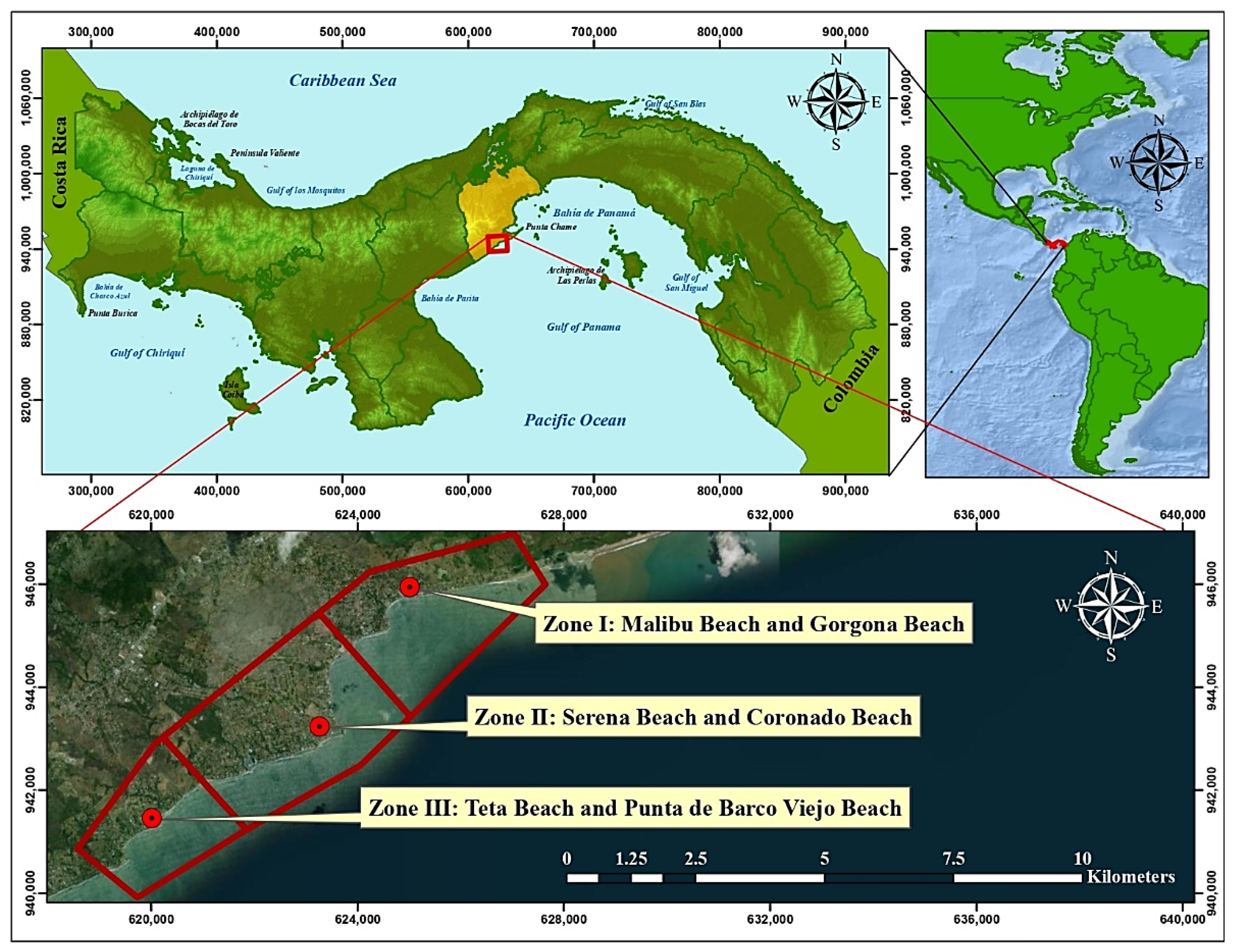
2.1. Study Zone

The Pacific Coast of Panama is one of the main tourist attractions in the country due to its proximity to the capital city, the shape of its sandy beaches, and the various recreational activities offered [30]. In this study, six beaches were selected, which were categorized into three zones (Figure 1), these being: zone I—Malibu beach and Gorgona beach, zone II—Serena beach and Coronado beach, and zone III—Teta beach and Punta Barco Viejo beach. The study zones are part of the province of Panamá Oeste, and the total length of the study line is approximately 11.80 km.

• Zone I—Malibu beach and Gorgona beach; This zone has a large residential development on the beachfront, in addition to the tall buildings that can be found in the zone. Some of the socioeconomic activities that take place in the zone are artisanal fishing, gastronomy, rental of vacation spaces, and surfing. The average orientation of the coast: Malibu beach ↙ WSW—Gorgona beach ↓ S to ↙ WSW.
• Zone II—Serena beach and Coronado beach; This zone was the first tourist development in the interior of Panama, with extensive commercial and residential development that generates jobs for the local population. The gastronomic variety, recreational activities, and beaches positioned it as one of the main tourist attractions in Panama. The average orientation of the coast: Serena beach ↓ S to ↘ SE—Coronado beach ↙ WSW.
• Zone III—Teta beach and Punta Barco Viejo beach; Its main attraction is the surfing activities for the waves in the zone because of the little residential and commercial development compared to the previous two. The average orientation of the coast: Teta beach ↙ SW—Punta Barco Viejo beach ↙ SW.

The study zone is characterized by an average annual temperature of 26.4 °C, waves of approximately 1.30 m in height, and a tropical climate with a prolonged dry season (

Table 1. General information about the study zone.

Tides	Tide levels are variable throughout the year on the Pacific coast of Panama. These tide levels can reach 6.00 m. The characteristic of the tides is semidiurnal, and the duration is a day of 24 h 50 min, and 25 s (lunar day) [37,38,39].
Waves	The wave data were obtained from the study for the port of Vacamonte (located at an approximate distance of 50.00 km) [40]. The wave frequency occurrence is around 60% between the S and WSW directions for the incident wave. The maximum height of the waves is 3.70 m, with a period of 15 s. The average height of the waves is 1.30 m with a period of 5.20 s.
Wind	The wind speed data at 2 m are published by the electrical transmission company ETESA, registered by the meteorological station located in Balboa, Panama. The average speed is 0.70 m/s for the dry season and 0.45 m/s for the rainy season [41].
Storms	The rainiest months on the Pacific coast of Panama correspond to September and October. According to ETESA, normally, the precipitation levels for the study zone during the rainy season reach a maximum of 2000 mm. During this season, there are frequent depressions and tropical storms. Contrary to the dry season, in which precipitation levels reach a maximum of 400 mm [42].

) [29]. Panama is a country that, due to its geographical position close to terrestrial Ecuador, the weather similar throughout the year at the national level. Only two seasons are identified: dry and rainy; the dry season extends from December to April, and the rainy season from the end of April to November [29].

Additionally, according to the geological characterization of the study zone, sedimentary formations belonging to the Quaternary are identified. These formations have materials made up of sandstone, shale, tuff, pumice stone, etc. On the other hand, the Lajas, Teta, and Chame rivers that flow into the beaches, present geological formations from the Tertiary. These show materials of volcanic origin are composed of dacites, lagoons, ignimbrite, pumice stone, andesites/basalts, etc. These materials are transported in the rivers, ending up in the surface currents parallel to the beach, which contributes to the composition of the sandy beach (Figure 2) [29].

The study zone is included in the “low coast” classification in which the elevations vary from 0–100 m, with a slope of 0° to 3°. Therefore, it is classified as part of the marine-coastal zones vulnerable to the consequences of climate change, such as extreme events (tidal waves) and the rise in mean sea level [29].

2.2. Materials

Optical satellite images from the Landsat missions were used in this study because they provide a greater number of images available for the research zone. In contrast, for the Sentinel 2-A satellite database, it was only found that the oldest image for the study zone corresponds to the year 2015. Landsat images were downloaded from the United States Geological Survey (U.S.G.S.) platform and are available for free access at: https://earthexplorer.usgs.gov/, accessed on 18 June 2022).

Landsat satellite images have provided multispectral images for the study zone since 1998 (the oldest image identified by the authors) with a resolution of 30 m pixels, acceptable for studies on a regional scale. Additionally, the selection of the satellite image of the year 1998 coincides with the series of years (1990–2000) in which the greatest urban development occurred along the beachfront in the study zone.

The search criteria correspond to the coordinate projection system “WGS 1984 UTM Zone 17N” and a cloud presence restriction of less than 15%. In addition, considering the climatic seasons for a tropical country such as Panama, only satellite images from the month of March (corresponding to the summer season) were selected (Section 2). This is to avoid the effects of hydrometeorological events (i.e., storms) typical of the winter season, in which the energy of the waves increases and the beach, in response, adopts a temporarily eroded form [43,44].

Based on these criteria, satellite images were obtained for an interval of 5–7 years from 1998 to 2022. This criterion was adopted to quantify the changes in the shoreline for the same season in a period greater than or equal to 5 years. The satellite images used are presented in Table 1.

On the other hand, within the limitations of this study, the effect of the variability of the tides is included. Due to the 30 m resolution of the pixel used, it is not possible to distinguish changes between tides (case similar to the research presented by Wicaksono (2018)) [45]. Additionally, it has been identified that there is a lack of information on in situ tides in the study zone and especially since they are free to access the Pacific coast of Panama.

Tidal data available for free access until the presentation of this study are provided by the NOA (National Oceanic and Atmospheric Administration) and the ACP (Autoridad del Canal de Panama), located at the Pacific entrance of the Panama Canal. These data have been available since 2008, so it was not possible to obtain information prior to this year. Additional information on monthly and yearly sea levels can be found on the PSMSL (Permanent Service for Mean Sea Level) website https://psmsl.org/data/obtaining/stations/163.php, accessed on 10 October 2022).

Table 2. Summary of data from the satellite images.

Information from Satellite Images
Satellite	Sensor	Path/Row	Acquisition Date	Hour	Spatial Resolution (Meters)	Tide Level (Approximation)
Landsat-5	TM	12/54	22 March 1998	15:12:44	30	-
Landsat-7	ETM+	12/54	30 March 2004	15:25:19	30	-
Landsat-7	ETM+	12/54	12 March 2009	15:26:11	30	Low to high (4.39 m)
Landsat-7	ETM+	12/54	15 March 2016	15:38:08	30	Low (0.52 m)
Landsat-8	OLI/TIRS	12/54	5 March 2021	15:35:46	30	Low (0.64 m)

Note: Thematic Mapper (TM), Enhanced Thematic Mapper (ETM), and Operational Land Imager (OLI)/Thermal Infrared Sensor (TIRS).

shows the information from the satellite images of the selected study zone and the approximate values of tides calculated using the indications in the NOAA tide table document.

2.3. Methods

2.3.1. Shoreline Extraction Methods

To carry out the shoreline extraction process, two methodologies were applied: Histogram Thresholding Method and Band Ratio Method.

In the Histogram Thresholding Method, a threshold must be defined in the histogram of band 5 (band 6 for Landsat 8). This must be given a maximum pixel value of “N” that divides the land from the water (Figure 3). With this, it will be possible to separate the values of “<N” that represent the water zones from the values “≥N” that represent the land zones (in

Table 3. Information about the spectral bands and N values used in the Histogram Thresholding Method.

Satellite	Band	Color	Wavelength (μm)	Observation	N Pixel Value in Histogram Threshold Method
Landsat-5	B2	Green	0.525–0.605
Landsat-5	B4	NIR	0.775–0.900
Landsat-5	B5	SWIR	1.550–1.750		30 (1998 year)
Landsat-7	B2	Green	0.519–0.601
Landsat-7	B4	NIR	0.772–0.898
Landsat-7	B5	SWIR	1.547–1.749		60 (2004 year), 75 (2009 year), 60 (2016 year)
Landsat-8	B3	Green	0.533–0.590	use in the position of band 2 *
Landsat-8	B5	NIR	0.851–0.879	use in the position of band 4 *
Landsat-8	B6	SWIR	1.566–1.651	use in the position of band 5 *	8000 (2021 year)

Note: use (*) in Equations (3) and (4).

, consult the N values used for each Landsat image) [25].

The image with the delimitation can be obtained quickly because water bodies absorb most of the radiation spectrum in the near-infrared band. In contrast, vegetation, sand, and other soil features have strong reflectance in the infrared bands [7,25].

To obtain the binary image, a reclassification was carried out based on the results obtained so that the values of 1 were associated with land (Equation (1)), and the values of 0 were associated with the values of water (Equation (2)). However, the misclassification of some pixels is one of the most important limitations in the application of this method. This is because pixels that represent land can be assigned as water. Therefore, this method has a high dependency on the level of user experience.

$$\mathrm{Values} \ge \mathrm{N} \to \mathrm{represent} \mathrm{land} \to \mathrm{reclassify} \to 1$$

(1)

$$\mathrm{Values} < \mathrm{N} \to \mathrm{represent} \mathrm{water} \to \mathrm{reclassify} \to 0$$

(2)

The second methodology is the Band ratio method. This method uses the reflectance associated with each of the objects captured in the image, which depending on their composition, will be greater or lesser in different spectral bands.

In the case of the study zone, the presence of sand, vegetation, artificial elements (i.e., buildings in general), and water was observed. The highest associated reflectance for the group of vegetation, artificial elements, and sand is observed in band 2 (green), band 4 (near infrared), and band 5 (mid-infrared) (the bands vary in the Landsat 8 OLI images/TIRS, see Table 3). In the case of water, there is an absorption of electromagnetic radiation, which distinguishes the boundary between land and water.

For Landsat-8 (OLI/TIRS) satellite images, a new spectral band has been included for coastal and aerosol studies (band 1). Therefore, to carry out the application of the Band Ratio Method, it is necessary to consider that the Landsat-8 bands are classified with another numbering. Table 3 includes information on the wavelength range associated with each satellite band.

The Band Ratio Method consists of two conditions corresponding to “Band (2)/Band (4)” Equation (3) and “Band (2)/Band (5)” Equation (4) were applied simultaneously, resulting in two binary images [21,25], where the pixels that had the value of 1 represented water and those that had values of 0 represented land. These two binary images were multiplied by each other to obtain a final binary image Equation (5).

Subsequently, to follow the classification code that had been made in the Histogram Thresholding Method, the final binary image was reclassified so that the pixels with a value of 1 took the value of 0, and pixels with a value of 0 took the value of 1.

$$\left\{ \frac{\mathrm{Band} \left(2\right)}{\mathrm{Band} \left(4\right)} \right\}=\mathrm{binary} \mathrm{image} 1$$

(3)

$$\left\{ \frac{\mathrm{Band} \left(2\right)}{\mathrm{Band} \left(5\right)} \right\}=\mathrm{binary} \mathrm{image} 2$$

(4)

$$\left\{\mathrm{binary} \mathrm{image} 1\right\}·\left\{ \mathrm{binary} \mathrm{image} 2 \right\}=\mathrm{binary} \mathrm{image} 3$$

(5)

When obtaining the binary images for each methodology, these were multiplied to obtain a final binary image that defined land and water zones. The raster image was converted to vector format. It is important to verify that the generated shoreline has been correctly extracted and smoothed to avoid very steep angles (Figure 4).

2.3.2. Uncertainty Assessment

The uncertainty values are related to the quality of the data used to generate the shorelines, the process applied to these data, and the characteristics of the environment when the data were recorded.

Therefore, the variables to consider to calculate the uncertainty in the total position (Ut) (Equation (6)) are the following: (1) seasonal error ($E_s$), which reduces the precision due to the occurrence of storms and waves; (2) error due to tidal fluctuations ($E_{td}$), which is related to changes in tide levels; (3) rectification error ($E_r$), which includes errors that can be generated when georeferencing the image; (4) error of digitization ($E_d$), which depends on the user’s skill in manual digitization processes (i.e., digitize the shoreline manually), and (5) pixel error ($E_p$), which is quantified when the images used have different resolutions [3].

$$U_{t_n}=\pm \sqrt{E_s{}^2+E_{td}{}^2+E_r{}^2+E_d{}^2+E_p{}^2}$$

(6)

$n$ represents the analyzed year.

To quantify the annualized uncertainty rate for the change in the shoreline in any analyzed transect [3]. The Equation (7) to use is the following:

$$U_a=\pm \frac{\sqrt{U_{t_{1998}}{}^2+U_{t_{2004}}{}^2+U_{t_{2009}}{}^2+U_{t_{2016}}{}^2+U_{t_{2021}}{}^2}}{total number of years}$$

(7)

Table 4. Summary of uncertainty estimates.

Estimation of Calculation Uncertainty
	1998	2004	2009	2016	2021	Observations
Seasonal error (Es) (m)	0	0	0	0	0	All the satellite images used correspond to the month of March in summer.
Tidal fluctuation error (Etd) (m)	0	0	0	0	0	Neglected due to resolution of satellite image.
Rectification error (Er) (m)	0	0	0	0	0	All satellite images have been orthorectified.
Digitizing error (Ed) (m)	30	30	30	30	30	According to the spatial resolution.
Pixel error (Ep) (m)	0	0	0	0	0	All the images used have the same spatial resolution.
Total uncertainty (Ut) (m)	30	30	30	30	30	All the images used have the same spatial resolution.
Annual uncertainty for a period of 23 years (m/year)	±2.92

shows the positional error calculated for each year of study, according to the data used as shown in Equations (6) and (7).

2.3.3. Digital Shoreline Analysis System (DSAS)

The Digital Shoreline Analysis System (DSAS) from the United States Geological Survey (U.S.G.S.) is a software that acts as an extension of ArcGIS-ArcMap, providing the arithmetic tools to quantify the evolution of the shoreline. The results it generates are obtained in terms of accretion or erosion rates (m/year) or the net movement on the shoreline (m) [46]. This tool is used to statistically calculate the shoreline change, using a time series of multiple shorelines in a defined range of years.

The input parameters necessary to execute the analysis of the evolution of the shoreline in the DSAS were the following: (1) two personal databases were established, corresponding to the shorelines and the baseline; (2) the database contained all the shorelines, including a field with the dates of each one in terms of month/day/year; (3) to generate the baseline a buffer was generated 100 m away from the 1998 shoreline (seaward); (4) the transects were generated in a length of 200 m because shorter distances generated transects that did not intersect some shorelines; and greater distances caused the transects to intersect each other at the most curved parts of the shorelines; (5) the distance between each transect was 20 m since a greater separation was not adequate due to the total length of the shoreline analyzed (11.80 km), and a smaller separation caused the transects to intersect each other in zones curves of the shoreline; (6) due to curved sections and transects intersected each other, a value of 200 was used for the “smoothing distance” tool; (7) the confidence interval used was 95%.

Finally, the baseline was in the offshore zone. Therefore, the movement of the shoreline if it moves towards land is considered erosion (−), and otherwise, the movement towards the sea is considered accretion (+) [27].

Long-Term Evolution of the Shoreline

The evolution of the shoreline was calculated using the Linear Regression Rate. This methodology fits the least squares regression line to all points on the shoreline for each transect. Linear regression rate change was calculated as change in shoreline slope; results are generated in units of m/year [4,5,47]. The calculated linear regression equation has the following form: L = b + mx, where; L represents the distance from the baseline in units of meters; x is the number of years being analyzed; m is the slope of the fitted line in units of m/year; b is the y-intercept.

The advantage of this method is that it uses all available information. For long-term analysis, it is the appropriate method because using a greater amount of data will improve the precision of the results. However, the disadvantage is that short-term calculations (i.e., changes between intermediate periods) are neglected [6].

The Net Shoreline Movement methodology was used to measure the distance between the oldest and the most recent shoreline for each transect Equation (8), providing results in units of meters [46,47]. The equation applied to each transect is as follows:

$$\mathrm{NSM}=\left(d_{2021}-d_{1998}\right) \mathrm{m}$$

(8)

Short-Term Evolution of the Shoreline

The End Point Rate methodology was used to analyze the evolution of the shoreline in the short term, that is, for the following groups of years: 1998–2004, 2004–2009, 2009–2016, and 2016–2021. This method consists of using the distance calculated by the net movement method (NSM) of the shoreline and dividing it into the time between the most recent and the oldest shoreline Equation (9). The results obtained by this method are in units of m/year. Its main advantages are flexibility and the fact that it only requires two shorelines. However, when using more than two shorelines, the intermediate information will be neglected [46]. The equation applied to each transect is the following:

$$\mathrm{EPR}=\left(\frac{d_{2021}-d_{1998}}{t_{2021}-t_{1998}}\right) \mathrm{m}/\mathrm{year}$$

(9)

Figure 5 presents the methodology used to carry out the analysis of the evolution of the shoreline on the beaches of the study zone. The flowchart includes (1) the data sources, (2) the automated shoreline extraction methods, and (3) the application of the Digital Shoreline Analysis System (DSAS).

3. Results

The shorelines generated by the automatic extraction methodology are presented in Figure 6. For which the long- and short-term changes will be analyzed by applying the statistical methods of the Digital Shoreline Analysis System (DSAS) software. The following sections show the results generated for the 23 years of study.

3.1. Long-Term Shoreline Evolution

The results obtained for the long-term analysis (LRR) are presented in

Table 5. Different classifications for change rates on the shoreline.

Category	Change Rate on the Shoreline (m/year)	Process Classification	Length (km)
1	>−2.00	Very high erosion	0.5
2	>−1.00 to <−2.00	High erosion	5.82
3	>0 to <−1.00	Moderate erosion	4.26
4	0	Stable	0
5	>0 to <+1.00	Moderate accretion	0.74
6	>+1.00 to <+2.00	High accretion	0.48
7	>+2.00	Very high accretion	0

, where positive values (+) reflect an accretion process on the beach, while negative values (−) indicate an erosion process. Out of the 11.80 km of shoreline analyzed, according to the results obtained, around 10.58 km of the shoreline presented erosion at different scales. The processes of erosion from high to very high classification occurred in an extension of 6.32 km, while the accretion processes were shown in 1.22 km, with categories ranging from moderate to high.

Zone I: the analyzed shoreline length of Malibu beach and Gorgona beach was approximately 4.24 km, obtaining results that indicate an erosion process. Additionally, only a small extension of the shoreline in Malibu beach exhibited accretion due to the proximity of the mouth of the Chame River (Figure 2). The maximum value recorded for accretion is 1.14 m/year. The erosive processes correspond to the category of moderate to high erosion, being accentuated in Gorgona beach (Figure 7). The maximum value recorded for erosion was −2.56 m/year. A total of 213 transects were generated at Malibu beach and Gorgona beach. Approximately 83.57% presented erosion, with an average movement of the shoreline was −24.17 m for negative distances. Approximately 16.43% of the total transects presented accretion, and the average movement of the shoreline was 24.46 m for positive distances.

Zone II: the zone of Serena beach and Coronado beach is the widest extension of shoreline length, with approximately 4.74 km analyzed. This zone shows an erosion process categorized as high in most of the extension of Serena beach (right section of the shoreline, Figure 8). This behavior was also exhibited along Coronado beach; however, a small extension of the shoreline presented accretion (left section of shoreline, Figure 8).

The maximum recorded value related to accretion is 1.39 m/year, with a total average value of 0.49 m/year. Additionally, the maximum registered erosion value corresponds to −2.31 m/year, with a total average of −1.01 m/year. In this zone, a total of 237 transects were used, of which 92.02% exhibited erosion and 7.98% accretion. The net movement of the shoreline (NSM) for negative distances registered a maximum value of −65.64 m, with an average value of −23.95 m. On the other hand, for positive distances, the maximum value of movement on the shoreline (NSM) obtained corresponds to 20.63 m, with a total average of 9.04 m.

Zone III: Teta beach and Punta Barco Viejo beach has a shoreline length of approximately 2.82 km. Its entire extension exhibits erosive processes that range from category of moderate to very high erosion. The section of the shoreline next to Teta beach presents a process of high, mostly uniform erosion (right section of the shoreline, Figure 9).

For the analysis of the net movement of the shoreline (NSM), the maximum value recorded for negative distances corresponds to −80.51 m (observed in zone III). In contrast, the maximum value recorded for positive distances corresponds to 31.60 m (observed in zone I). However, it is important to note that the values mentioned were calculated in transects that are close to the mouths of rivers. The contribution of sediments from river channels can influence the results recorded in nearby transects (Figure 2). Figure 10 presents the total movement of the shoreline for the time interval between 1998 and 2021.

The analyses applied for the long-term in the study zone contribute to determining the erosion process. This can be deduced from the results presented in

Table 6. Summary of the results obtained for the long-term analysis.

Summary of Long-Term Analysis, 1998–2021	Zone I	Zone II	Zone III
General information
Transect range	1–213	214–451	452–593
Total transects	213	237	141
Shoreline length (km)	4.24	4.74	2.82
Net Shoreline Movement (NSM)
% of transects that presented erosion	83.57	92.02	96.48
% of transects that presented accretion	16.43	7.98	3.52
Maximum negative distance (m)	−52.54	−65.64	−80.51
Maximum positive distance (m)	31.60	20.63	5.96
Average of all negative distances (m)	−24.17	−23.95	−23.43
Average of all positive distances (m)	24.46	9.04	3.12
Linear Regression Rate (LRR)
Maximum erosion value (m/year)	−2.56	−2.31	−3.09
Maximum accretion value (m/year)	1.14	1.39	0.08
Average of all erosion rates (m/year)	−1.12	−1.01	−1.08
Average of all accretion rates (m/year)	0.92	0.49	0.07

, in which the average erosion and accretion rates for each of the zones are shown.

However, it is necessary to identify if it has been produced by natural or anthropogenic causes or has been derived from the consequences of climate change. Therefore, the short-term analysis provides more detailed information on the changes experienced in pairs of years.

3.2. Short-Term Shoreline Evolution

Zone I: according to the results obtained for the short-term analysis, the maximum erosion rate has a value of −12.85 m/year and an average value of −2.68 m/year for the range between 2004–2009. Instead, the value of the maximum accretion rate corresponds to 11.46 m/year, with an average value of 2.56 m/year recorded for 2016–2021 (Figure 11).

The average value of erosion recorded for the years 2004–2009 is the second highest of those recorded in the three study zones. Additionally, during these years, some publications were made in national newspapers of Panama that indicated sand extraction in the zone, which could influence the evolution of the shoreline.

On the other hand, the average value of accretion obtained between 2016 and 2021 for this zone was the second highest recorded in the analysis. The contribution of sediments by the Chame River could also have an influence since the transects where the accretion values were recorded were located close to the mouth of the river.

Zone II: the maximum erosion rate is −8.67 m/year, with an average value of −1.91 m/year recorded for the study between 2016 and 2021. Instead, the maximum accretion rate has a value of 6.88 m/year and an average value of 2.29 m/year corresponding to 2004–2009 (Figure 12).

The zone of Serena beach and Coronado beach was one of the first tourist zones developed in the interior of the country. From 1990, its popularity increased, being a residential attraction for nationals and foreigners. However, the beach zone was reducing its extension, causing the waves to get closer to private properties, as indicated in local newspapers. These factors could have affected the shoreline of the beach (according to erosion data for 2004–2009).

Zone III: the maximum erosion rate has a value of −14.06 m/year and an average value of −3.39 m/year for the range between 2004 and 2009. Instead, the value of the maximum accretion rate corresponds to 12.36 m/year, with an average value of 2.68 m/year, also recorded for 2004–2009 (Figure 13).

The zone of Teta beach and Punta Barco Viejo beach, despite being a zone with low population density and economic activities, experiences the highest rates of erosion. However, the accretion rates showed favorable values compared to zone II. The influence of coastal protection structures near Punta Barco Viejo beach and the contribution of sediments by the fluvial channel are objects for future studies of the evolution of the shoreline.

Table 7. Summary of the results obtained for the short-term analysis.

Short-Term Analysis Summary (End Point Rate, EPR)	1998–2004	2004–2009	2009–2016	2016–2021
Zone I—Malibu beach and Gorgona beach
% of transects that presented erosion	64.32	90.14	70.28	51.89
% of transects that presented accretion	35.68	9.68	29.72	48.11
Maximum erosion value (m/year)	−11.29	−12.85	−5.05	−4.70
Maximum accretion value (m/year)	4.14	4.66	8.32	11.46
Average of all erosion rates (m/year)	−2.00	−2.68	−1.68	−1.54
Average of all accretion rates (m/year)	1.45	2.01	2.47	2.56
Zone II—Serena beach and Coronado beach
% of transects that presented erosion	91.60	47.48	67.65	66.81
% of transects that presented accretion	8.40	52.52	32.35	33.19
Maximum erosion value (m/year)	−4.44	−8.56	−4.91	−8.67
Maximum accretion value (m/year)	3.37	6.88	5.63	5.18
Average of all erosion rates (m/year)	−2.05	−2.44	−1.92	−1.91
Average of all accretion rates (m/year)	0.76	2.29	1.12	1.37
Zone III—Teta beach and Punta Barco Viejo beach
% of transects that presented erosion	64.08	73.24	71.13	52.82
% of transects that presented accretion	35.92	26.76	28.87	47.18
Maximum erosion value (m/year)	−7.78	−14.06	−8.74	−5.31
Maximum accretion value (m/year)	8.13	12.36	3.89	4.75
Average of all erosion rates (m/year)	−2.37	−3.39	−2.27	−2.27
Average of all accretion rates (m/year)	1.86	2.68	1.83	2.09

shows the results obtained for the analysis developed in the short term through the End Point Rate analysis. This shows the maximum rates of erosion and accretion recorded in a transect for each specific zone. The average recorded erosion and accretion rates are also indicated.

4. Discussion

4.1. Accuracy Assessment of the Shoreline Extraction Method

The accuracy of the method used to extract the shorelines was evaluated by digitizing a high-resolution satellite image (<1.00 m) obtained from the Google Earth Pro historical viewer for the study zone. The available extracted image corresponded to the year 2022 since no available images were found for the year 2021. The image used corresponds to the summer season (February) since the climatic conditions between the months of January–March for the study zone are very similar and where storms do not normally occur.

Additionally, the automatic extraction of another shoreline was carried out from a Landsat 8 OLI/TIRS satellite image from February. This was compared with shoreline of the high-resolution image of Google Earth Pro using the DSAS by analyzing the Shoreline Change Envelope (SCE) that measures the distance between shoreline lines. For this process, a total of 603 transects were used, with a length of 200 m and 20 m of space between each one. The baseline used was generated by a buffer of 100 m (seaward) from the manually digitized shoreline.

The results obtained from the transects show that 60% of the distance between both shorelines is ≤8.00 m, which is considered favorable due to the difference in resolution between both images (Figure 14). However, within the 40% that exceeds >8.00 m, they are identified in sections of the shoreline that have a curved shape. This would indicate a limitation of the methodology to be applied to shorelines that have curved shapes since their best performance is identified in relatively straight zones (Figure 15).

On the other hand, Alesheikh et al. (2017) indicate that the methodology that combines the Histogram Thresholding Method and the Band Ratio Method (used in this study) to extract the shoreline allows for obtaining better results than using the methods separately, but the limitation of this method is that some sections of the shoreline will be misclassified since the line could be towards the seaward (Figure 16). Therefore, if the main interest is to obtain the rapid extraction of the coastline, this will be an appropriate method; on the contrary, if precision is required, it will present some limitations [19].

According to the analysis of the precision of the shoreline extraction method, it can be indicated that the average error associated with the results obtained, shown in Figure 14, was quantified by means of the root mean square error ($RMSE$) (Equation (10)), where Δ is the error measured for each element and $n$ is the total number of elements. The mean square error ($RMSE$) obtained for the results is ±6.39 m, this result represents less than 1/3 pixel, so it is considered acceptable.

$$RMSE=\pm \sqrt{\frac{{\displaystyle \sum }\left|\left({\Delta }_1{}^2\right)\right|+\left|\left({\Delta }_2{}^2\right)\right|+\dots +\left|\left({\Delta }_{n-1}{}^2\right)\right|+\left|\left({\Delta }_n{}^2\right)\right|}{n}}$$

(10)

Additionally, the data published by Luijendijk et al. 2018 present a global erosion analysis on sandy beaches, providing a freely accessible tool for querying the results (http://shorelinemonitor.deltares.nl, accessed on 29 October 2022) [48]. In the consultation on this site, it has been observed that some transects and the results obtained in this study coincide.

Therefore, for this case study, the performance of the shoreline extraction methodology is considered acceptable since the standard deviation is much lower than the resolution of the satellite image used (for the accuracy test described above). However, due to the resolution used, it is also important to consider that the results of rates should be used carefully. These values need to be compared with studies that use high-resolution images and data obtained in situ.

4.2. Analysis of Beach Erosion in the Study Zone

In general, this study provides quantitative information on the evolution of the shoreline in the convergence zone of the Gulf of Panama. In conjunction with the qualitative information available in the literature, it indicates that visually there is an erosion process that has progressed over time, affecting the inhabitants and properties. However, to the knowledge of the authors, there is no information available to determine the main cause that contributes to this deterioration (i.e., natural or anthropic).

The results obtained in this study and the review of the literature provide information to identify the factors that have contributed to the changes in the shoreline. In general, these factors can be anthropogenic (e.g., beachfront construction, coastal engineering structures, sand extraction, etc.) or natural (e.g., tides, waves, etc.).

Zone I (Malibu beach and Gorgona beach) presents the highest erosion rates for the study period between 2004 and 2009; this coincides with the construction of houses and buildings on the beachfront (which extends until the period of 2009–2016). In addition, the problem of sand extraction and the construction of terraces deteriorated the natural defenses of the beach (i.e., dunes) [34,49,50]. Therefore, visible erosion seems to have its origin in anthropogenic causes, although it is also important to pay attention to the convergence of the waves and their associated energy [31].

These factors are also identified in zone II (Serena beach and Coronado beach), gaining greater importance because it is the study zone with the highest population density. The Serena beach zone has a more critical situation compared to Coronado beach since it was observed that the beach zone is narrower [35,36]. Additionally, in this zone, diffraction of the incident waves occurs since the waves that arrive with a WSW orientation collide 60% of the time with the formation of outgoing land called Punta Prieta. Therefore, the southern orientation of Serena beach could cause the transported sediment to be less on this beach compared to the adjacent beaches.

In general, Serena beach and Coronado beach, during the years 1990–2016, was the period in which the constructions on the beachfront intensified, possibly affecting the beach zone. In the case of Coronado beach, a wider beach zone was observed, except in front of some properties where the width of the beach is narrow and which can be more affected during high tides (and strong waves).

In zone III (Teta beach and Punta Barco Viejo beach), cliff-type formations were identified on the coastline that shows erosion due to waves and tidal variations in the zone. The residents of these zones have also built terraces to protect their properties. Some of these terraces include “boulder barriers”, due to the energy with which the waves can impact. On the other hand, some cliffs seem to have mechanical stabilization treatments to prevent erosion processes.

The supply of sediments in this zone depends largely on the river, so the dry seasons upstream influence the balance of the beach. Additionally, in this and nearby zones, extraction of sand by barges and heavy vehicles has been reported. This contributes to the concern for residents with modest houses that are located near the beach since they are forced to move their homes to avoid being affected by waves and tides [51,52].

The three study zones do not have coastal structures such as breakwaters or breakwaters; however, some sections of Serena beach have boulders located that simulate groynes. The closest breakwater to the zone is 5 km from Punta Barco Viejo beach, where an accumulation of sediment can be seen in the eastern part of the breakwater (Figure 17). These sediments accumulate in the sheltered zone of the breakwater, which hinders their transport to nearby beaches (which are the subject of this study).

Other possible causes of coastal erosion in these zones are related to (1) the occurrence of “swell”, in which waves can reach heights of 3.00 m, (2) variations in wave patterns due to storms and tropical depressions (which occur mostly in the winter season), (3) climatic variations related to the “El Niño” phenomenon, which in the Panamanian Pacific region generates a decrease in precipitation levels [53].

The information available in the literature (e.g., articles, newspapers, and official sites of national entities of Panama) and observation tools such as Google Earth Pro and Google Street View (available from August 2022 for the study zones), it is possible to gather the information that shows the problem of beach erosion in the Pacific of Panama. However, due to the limitations of this study, it is not possible to establish the main cause of coastal erosion during the study period. The factors that have possibly contributed to the evolution of the shorelines identified in this study are presented in Figure 18.

5. Conclusions

Coastal erosion in the region of the Pacific coast of Panama has been a very little studied topic, despite the concern expressed by the inhabitants of these zones. The loss of the beach zone has contributed to the strong waves generated in the region between Malibu beach and Punta Barco Viejo beach, reaching buildings such as houses and terraces, which could be more affected in a future scenario of climate change.

The lack of available information that quantifies the loss of the beach line and that includes the possible factors that contribute to this change is one of the main knowledge gaps detected when carrying out this study. Therefore, the results obtained and their subsequent interpretation provide a better idea of the evolution of the shoreline in order to develop studies in greater detail and precision in the future in one of the most developed coastal zones in the interior of Panama.

The selection of the data used in this study was considered with the criterion that they were freely accessible and that they allowed access to a historical record. Within the category of multispectral satellite imagery, the authors only identified Landsat imagery as meeting both requirements. Additionally, it was decided that the availability of the images from the year (1998) coincided with the period in which urban development was accelerated.

The automatic shoreline extraction method applied to the selected satellite images allowed obtaining results considered favorable (RMSE = ±6.39 m in the accuracy test), despite the 30 m resolution of the satellite images used. However, it is important to understand that the erosion rates presented should be used carefully due to the limitations of this study. In the case of needing information to implement strategies in the zone, a previous study must be carried out that uses in situ information and high-resolution images.

The changes in the shoreline indicate that there is a general erosion process; the zones most exposed to the risks of this process are Serena beach and Coronado beach. Additionally, the southern orientation of Serena beach with respect to nearby beaches contributes to the erosion process because the waves, when advancing in Coronado beach (in a WSW to S direction), reach Punta Prieta, generating wave diffraction in Serena beach.

The average erosion and accretion values obtained by the DSAS with the LRR method for the period between 1998 and 2021 correspond to Zone I with −1.12/+0.92 m/year, Zone II with −1.01/+0.49 m/year, and Zone III with −1.08/+0.07 m/year. These values were obtained by analyzing the shorelines extracted for the month of March during the summer season in Panama because during the winter season, in addition to the variability of hydrodynamic conditions, events such as storms and tropical depressions sometimes occur.

The methodology applied in this study can be replicated in other zones of Panama that have coastal erosion problems. An example of this is the zone of Punta Chame [54,55], which has been identified as at risk of erosion and has similar characteristics in terms of urban development and sand extraction problems. The joint efforts of the study of coastal erosion in the wave convergence zone in the Gulf of Panama would assist decision makers in the development of local management and coastal management plans.

References

1. Baral, R.; Pradhan, S.; Samal, R.N.; Mishra, S.K. Shoreline Change Analysis at Chilika Lagoon Coast, India Using Digital Shoreline Analysis System. J. Indian Soc. Remote Sens. 2018, 46, 1637–1644. [Google Scholar] [CrossRef]
2. Baig, M.R.I.; Ahmad, I.A.; Shahfahad; Tayyab, M.; Rahman, A. Analysis of Shoreline Changes in Vishakhapatnam Coastal Tract of Andhra Pradesh, India: An Application of Digital Shoreline Analysis System (DSAS). Ann. GIS 2020, 26, 361–376. [Google Scholar] [CrossRef]
3. Vu, M.T.; Lacroix, Y.; Than, V.V.; Viet Thanh, N.; Nguyen, T. Prediction of Shoreline Changes in Almanarre Beach Using Geospatial Techniques. Indian J. Geo-Mar. Sci. 2020, 49, 207–217. [Google Scholar]
4. Jayson-Quashigah, P.-N.; Addo, K.A.; Kodzo, K.S. Medium Resolution Satellite Imagery as a Tool for Monitoring Shoreline Change. Case Study of the Eastern Coast of Ghana. J. Coast. Res. 2013, 65, 511–516. [Google Scholar] [CrossRef]
5. Franco-Ochoa, C.; Zambrano-Medina, Y.; Plata-Rocha, W.; Monjardín-Armenta, S.; Rodríguez-Cueto, Y.; Escudero, M.; Mendoza, E. Long-Term Analysis of Wave Climate and Shoreline Change along the Gulf of California. Appl. Sci. Switz. 2020, 10, 8719. [Google Scholar] [CrossRef]
6. Yasir, M.; Sheng, H.; Fan, H.; Nazir, S.; Niang, A.J.; Salauddin, M.; Khan, S. Automatic Coastline Extraction and Changes Analysis Using Remote Sensing and GIS Technology. IEEE Access 2020, 8, 180156–180170. [Google Scholar] [CrossRef]
7. Santos, C.A.G.; do Nascimento, T.V.M.; Mishra, M.; da Silva, R.M. Analysis of Long- and Short-Term Shoreline Change Dynamics: A Study Case of João Pessoa City in Brazil. Sci. Total Environ. 2021, 769, 144889. [Google Scholar] [CrossRef]
8. Velsamy, S.; Balasubramaniyan, G.; Swaminathan, B.; Kesavan, D. Multi-Decadal Shoreline Change Analysis in Coast of Thiruchendur Taluk, Thoothukudi District, Tamil Nadu, India, Using Remote Sensing and DSAS Techniques. Arab. J. Geosci. 2020, 13, 838. [Google Scholar] [CrossRef]
9. Natarajan, L.; Sivagnanam, N.; Usha, T.; Chokkalingam, L.; Sundar, S.; Gowrappan, M.; Roy, P.D. Shoreline Changes over Last Five Decades and Predictions for 2030 and 2040: A Case Study from Cuddalore, Southeast Coast of India. Earth Sci. Inform. 2021, 14, 1315–1325. [Google Scholar] [CrossRef]
10. Mutaqin, B.W. Shoreline Changes Analysis in Kuwaru Coastal Area, Yogyakarta, Indonesia: An Application of the Digital Shoreline Analysis System (DSAS). Int. J. Sustain. Dev. Plan. 2017, 12, 1203–1214. [Google Scholar] [CrossRef]
11. Seisdedos, J.; Mulas, J.; de Vallejo, L.I.G.; Franco, J.A.R.; Gracia, F.J.; del Río, L.; Garrote, J. Estudio y Cartografía de Los Peligros Naturales Costeros de La Región de Murcia. Boletín Geológico Min. 2014, 124, 505–520. [Google Scholar]
12. United States Geological Survey (USGS). Landsat Satellite Missions. Landsat Missions. Available online: https://www.usgs.gov/ (accessed on 18 June 2022).
13. Sentinel. Sentinel Overview. Sentinel Online—European Space Agency. Available online: https://sentinel.esa.int/web/sentinel/missions (accessed on 7 November 2022).
14. Pardo-Pascual, J.E.; Sánchez-García, E.; Almonacid-Caballer, J.; Palomar-Vásquez, J.M.; Priego de los Santos, E.; Fernández-Sarría, A.; Balaguer-Beser, Á. Assessing the Accuracy of Automatically Extracted Shorelines on Microtidal Beaches from Landsat 7, Landsat 8 and Sentinel-2 Imagery. Remote Sens. 2018, 10, 326. [Google Scholar] [CrossRef]
15. Mirsane, H.; Maghsoudi, Y.; Rohollah, E.; Mostafavi, M. Automatic Coastline Extraction Using Radar and Optical Satellite Imagery and Wavelet-IHS Fusion Method. Int. J. Coast. Offshore Eng. 2018, 2, 11–20. [Google Scholar] [CrossRef] [Green Version]
16. Čotar, K.; Oštir, K.; Kokalj, Ž. Radar Satellite Imagery and Automatic Detection of Water Bodies. Geod. Glas. 2016, 50, 5–15. [Google Scholar]
17. García-Rubio, G.; Huntley, D.; Esteves, L. Shoreline Identification Using Satellite Images. Coast. Dyn. 2009, 2009, 1–10. [Google Scholar] [CrossRef]
18. Alcaras, E.; Errico, A.; Falchi, U.; Parente, C.; Vallario, A. Coastline Extraction from Optical Satellite Imagery and Accuracy Evaluation. In International Workshop on R3 in Geomatics: Research, Results and Review; Springer: Naples, Italy, 2020. [Google Scholar]
19. Alesheikh, A.A.; Ghorbanali, N.N. Coastline Change Detection Using Remote Sensing. Int. J. Environ. Sci. Technol. 2017, 4, 61–66. [Google Scholar] [CrossRef] [Green Version]
20. Huang, C.; Wylie, B.; Yang, L.; Homer, C.; Zylstra, G. Derivation of a Tasselled Cap Transformation Based on Landsat 7 At-Satellite Reflectance. Int. J. Remote Sens. 2002, 23, 1741–1748. [Google Scholar] [CrossRef]
21. Nassar, K.; Mahmod, W.E.; Fath, H.; Masria, A.; Nadaoka, K.; Negm, A. Shoreline Change Detection Using DSAS Technique: Case of North Sinai Coast, Egypt. Mar. Georesour. Geotechnol. 2019, 37, 81–95. [Google Scholar] [CrossRef]
22. Gómez-Pazo, A.; Payo, A.; Paz-Delgado, M.V.; Delgadillo-Calzadilla, M.A. Open Digital Shoreline Analysis System: ODSAS v1.0. J. Mar. Sci. Eng. 2021, 10, 26. [Google Scholar] [CrossRef]
23. Jackson, C.W., Jr.; Alexander, C.R.; Bush, D.M. Application of the AMBUR R Package for Spatio-Temporal Analysis of Shoreline Change: Jekyll Island, Georgia, USA. Comput. Geosci. 2012, 41, 199–207. [Google Scholar] [CrossRef]
24. Terres de Lima, L.; Fernández-Fernández, S.; Marcel de Almeida Espinoza, J.; da Guia Albuquerque, M.; Bernardes, C. End Point Rate Tool for QGIS (EPR4Q): Validation Using DSAS and AMBUR. Int. J. Geo-Inf. 2021, 10, 162. [Google Scholar] [CrossRef]
25. Kafrawy, S.; Basiouny, M.; Ghanem, E.; Taha, A. Performance Evaluation of Shoreline Extraction Methods Based on Remote Sensing Data. J. Geogr. Environ. Earth Sci. Int. 2017, 11, 1–18. [Google Scholar] [CrossRef]
26. Kankara, R.S.; Selvan, S.C.; Markose, V.J.; Rajan, B.; Arockiaraj, S. Estimation of Long and Short Term Shoreline Changes along Andhra Pradesh Coast Using Remote Sensing and GIS Techniques. In Procedia Engineering; Elsevier Ltd.: Amsterdam, The Netherlands, 2015; Volume 116, pp. 855–862. [Google Scholar]
27. Bheeroo, R.A.; Chandrasekar, N.; Kaliraj, S.; Magesh, N.S. Shoreline Change Rate and Erosion Risk Assessment along the Trou Aux Biches–Mont Choisy Beach on the Northwest Coast of Mauritius Using GIS-DSAS Technique. Environ. Earth Sci. 2016, 75, 444. [Google Scholar] [CrossRef]
28. Dupar, M.; Pacha, M.J. IPCC’s Special Report on the Ocean and Cryosphere in a Changing Climate: What’s in it for Latin America? Climate and Development Knowledge Network: Cape Town, South Africa, 2019. [Google Scholar]
29. Panamá, Ministerio de Ambiente. Atlas Ambiental de Panamá. 2010. Available online: https://www.sinia.gob.pa/index.php/atlas-ambientales (accessed on 25 June 2022).
30. Panamá, Autoridad de Turismo de Panamá. Plan Maestro de Turismo Sostenible de Panamá 2020–2025. 2020. Available online: https://www.atp.gob.pa/Plan_Maestro_de_Turismo_Sostenible_2020-2025.pdf (accessed on 25 June 2022).
31. Grimaldo, A.M.O. Plano de Las Olas Del Golfo de Panamá. Tecnociencia—Univ. Panamá 2014, 16, 55–63. Available online: https://revistas.up.ac.pa/index.php/tecnociencia/article/download/1191/1002/1969 (accessed on 5 November 2022).
32. Piragua—Fuego y Agua: Vulnerabilidad Zonas Costeras. Piragua—Fuego y agua. Available online: https://piraguamdp.com/tag/vulnerabilidad-zonas-costeras/ (accessed on 2 November 2022).
33. Diéguez Pinto, M. Piragua—Fuego y Agua: Informe Sobre La Gira a La Zona Costera de Punta Chame. Piragua—Fuego y agua. 2020. Available online: https://piraguamdp.com/2020/04/14/informe-sobre-la-gira-a-la-zona-costera-de-punta-chame/ (accessed on 2 November 2022).
34. Diéguez Pinto, M. Piragua—Fuego y Agua: Informe de Gira a La Zona Costera de Nueva Gorgona. Piragua—Fuego y agua. 2020. Available online: https://piraguamdp.com/2020/04/14/informe-de-gira-a-la-zona-costera-de-nueva-gorgona/ (accessed on 2 November 2022).
35. Reyna Aparicio, J.D. La Estrella de Panamá—Frente de Playa y Rompiente En Peligro. La Estrella de Panamá, Panamá. 2017. Available online: https://www.laestrella.com.pa/cafe-estrella/planeta/170620/playa-frente-peligro-rompiente (accessed on 2 November 2022).
36. Arellano Lennox, C. La Prensa—El Enemigo Más Peligroso de La Playa de Coronado. La Prensa, Panamá. 2004. Available online: https://www.prensa.com/impresa/opinion/peligroso-Coronado-Carlos-Arellano-Lennox_0_1286871404.html (accessed on 2 November 2022).
37. NOAA—Historic Tide and Tidal Currents Tables. NOAA—Tides and Currents. Available online: https://www.tidesandcurrents.noaa.gov/historic_tide_tables (accessed on 30 October 2022).
38. Autoridad del Canal de Panamá. Canal de Panamá—Tabla de Mareas 2022. Canal de Panamá. Available online: https://pancanal.com/es/servicios-maritimos/mas-informacion/ (accessed on 30 October 2022).
39. Kirkpatrick, R.Z. Panama Tidal Differences. Int. Hydrogr. Rev. 1932. Available online: https://core.ac.uk/download/pdf/268174985.pdf (accessed on 30 October 2022).
40. Japan International Cooperation Agency: Pacific Consultants International. El Estudio Sobre El Plan de Desarrollo Integral de Puertos En La República de Panamá. 2004. Available online: https://openjicareport.jica.go.jp/728/728/728_618_11772100.html (accessed on 6 November 2022).
41. ETESA—Datos Climáticos Históricos. ETESA—Hidrometeorología. Available online: https://www.hidromet.com.pa/es/clima-historicos (accessed on 31 October 2022).
42. ETESA—Régimen Pluviómetrico de Panamá. ETESA—Hidrometeorología. Available online: https://www.hidromet.com.pa/es/regimen-pluviometrico-panama (accessed on 31 October 2022).
43. United States Army Corps of Engineers. Shore Protection Manual; Coastal Engineering Research Center; United States Army Corps of Engineers: Washington, DC, USA, 1984. [Google Scholar]
44. Sánchez-Arcilla, A.; Jiménez, J.A. Ingeniería de Playas (I): Conceptos de Morfología Costera. Ing. Del Agua 1994, 1, 97. [Google Scholar] [CrossRef] [Green Version]
45. Wicaksono, A.; Wicaksono, P.; Khakhim, N.; Farda, N.M.; Aris Marfai, M. Tidal Correction Effects Analysis on Shoreline Mapping in Jepara Regency. J. Appl. Geospatial Inf. 2018, 2, 145. [Google Scholar] [CrossRef]
46. Himmelstoss, E.A.; Henderson, R.E.; Kratzmann, M.G.; Farris, A.S. Digital Shoreline Analysis System (DSAS) Version 5.0 User Guide; Open-File Report 2018–1179; U.S. Geological Survey: Woods Hole, MA, USA, 2018; 110p. [CrossRef] [Green Version]
47. Dewidar, K.; Bayoumi, S. Forecasting Shoreline Changes along the Egyptian Nile Delta Coast Using Landsat Image Series and Geographic Information System. Environ. Monit. Assess. 2021, 193, 429. [Google Scholar] [CrossRef]
48. Luijendijk, A.; Hagenaars, G.; Ranasinghe, R.; Baart, F.; Donchyts, G.; Aarninkhof, S. The State of the World’s Beaches. Sci. Rep. 2018, 8, 6641. [Google Scholar] [CrossRef]
49. Montenegro, E. Crítica—Extracción Ilegal de Arena En Playas de Gorgona En Chame. Crítica, Panamá. 2006. Available online: https://portal.critica.com.pa/archivo/11162006/prov01.html (accessed on 7 November 2022).
50. Santos, J.V.A. Panamá América—Sigue Extracción Ilegal de Arena En Oeste. Panamá América, Panamá. 2004. Available online: https://www.panamaamerica.com.pa/provincias/sigue-extraccion-ilegal-de-arena-en-oeste-176822 (accessed on 7 November 2022).
51. Crítica—Barcaza Bruja Extrae Arena Ilegalmente En El Oeste. Crítica, Panamá. 2003. Available online: https://portal.critica.com.pa/archivo/11182003/cie02.html (accessed on 8 November 2022).
52. Diéguez Pinto, M. Piragua—Informe de Gira a Zona Costera—Playa de La Ensenada En San Carlos. Piragua—Fuego y agua. Available online: https://piraguamdp.com/2018/11/07/informe-de-gira-a-zona-costera-playa-de-la-ensenada-en-san-carlos/ (accessed on 5 November 2022).
53. ETESA Panamá. ETESA—El Fenómeno de El Niño y Sus Efectos en Panamá. ETESA—Hidrometeorología. Available online: https://www.hidromet.com.pa/es/documentos/fenomeno-el-nino (accessed on 7 November 2022).
54. Diéguez Pinto, M. Piragua—Desgaste En La Zona Costera de Punta Chame, Panamá. Piragua—Fuego y agua. 2020. Available online: https://piraguamdp.com/2020/05/05/desgaste-en-la-zona-costera-de-punta-chame-panama/ (accessed on 2 November 2022).
55. Guevara, T.J.M.; Douglas, A.I.; García-Maraña, K.; Barria, Y. Determinación de Riesgos de Desastres e Incidencia Del Cambio Climático En La Comunidad de Punta Chame, Panamá. Rev. Iniciación Científica 2022, 8, 24–31. [Google Scholar] [CrossRef]
Figure 1. Map of the study zone located on the Pacific Coast of Panama.
Jmse 10 01801 g001
Figure 2. Geological, hydrological, and coast of study zones. Cartography made by Smithsonian Tropical Research Institute.
Jmse 10 01801 g002
Figure 3. Histogram Thresholding Method process.
Jmse 10 01801 g003
Figure 4. Automatic shoreline extraction process.
Jmse 10 01801 g004
Figure 5. Applied methodology for the analysis of the evolution of the shoreline.
Jmse 10 01801 g005
Figure 6. Shorelines extracted for the study years.
Jmse 10 01801 g006
Figure 7. Erosion or accretion rates and profiles obtained by analyzing zone I by applying the Linear Regression Rate (LRR) for the period from 1998 to 2021.
Jmse 10 01801 g007
Figure 8. Erosion or accretion rates and profiles obtained by analyzing zone II by applying the Linear Regression Rate (LRR) for the period from 1998 to 2021.
Jmse 10 01801 g008
Figure 9. Erosion or accretion degrees and profiles obtained by analyzing zone III by applying the Linear Regression Rate (LRR) for the period from 1998 to 2021.
Jmse 10 01801 g009
Figure 10. Net shoreline movement (NSM) recorded for each transect for the period from 1998 to 2021.
Jmse 10 01801 g010
Figure 11. Accretion and erosion profiles obtained in zone I by applying the End Point Rate (EPR).
Jmse 10 01801 g011
Figure 12. Accretion and erosion profiles obtained in zone II by applying the End Point Rate (EPR).
Jmse 10 01801 g012
Figure 13. Accretion and erosion profiles obtained in zone III by applying the End Point Rate (EPR).
Jmse 10 01801 g013
Figure 14. Analysis of the accuracy of shoreline extraction method.
Jmse 10 01801 g014
Figure 15. Distance between shoreline of the High-Resolution image vs. shoreline of Medium Resolution image.
Jmse 10 01801 g015
Figure 16. Misclassified pixels. Dashed line = shoreline digitized manually from Google earth pro. Solid line = shoreline automatically extracted from Landsat image.
Jmse 10 01801 g016
Figure 17. Breakwater zone (red circle) located approximately 5 km away from Punta Barco Viejo Beach (yellow rectangle). The presence of two breakwaters (blue triangle) near the breakwater is observed. Images used from the historical viewer of Google Earth Pro.
Jmse 10 01801 g017
Figure 18. Upper image: factors with possible influence on shoreline change. Lower image: waves map adapted from Grimaldo (2014).
Jmse 10 01801 g018