Article

Branch-And-Price Algorithm for the Tramp Ship Routing and Scheduling Problem Considering Ship Speed and Payload

1
Rail Data Research and Application Key Laboratory of Hunan Province, School of Traffic & Transportation Engineering, Central South University, Changsha 410075, China
2
School of Traffic & Transportation Engineering, Central South University, Changsha 410075, China
3
School of Engineering, Center for Advanced Design and Engineering Training, Deakin University, Waurn Ponds, Geelong, VIC 3216, Australia
*
Author to whom correspondence should be addressed.
J. Mar. Sci. Eng. 2022, 10(12), 1811; https://doi.org/10.3390/jmse10121811
Submission received: 24 October 2022 / Revised: 18 November 2022 / Accepted: 21 November 2022 / Published: 23 November 2022
(This article belongs to the Section Ocean Engineering)

Abstract

:
In recent years, increasing fuel prices, depressed market conditions and air pollution issues have brought huge challenges to the tramp shipping industry. This work investigates the tramp ship routing and scheduling problem considering ship speeds and payloads, aiming at minimizing ship fuel consumption. A mixed integer non-linear programming model with a discretized speed variable and a set partitioning model for this problem is established, and a branch-and-price algorithm is proposed to solve the problem. Through the column generation approach, the problem at each branch-and-bound node is decomposed into a linear programming master problem and a pricing problem of the elementary shortest path with resource constraints. A labeling algorithm is adopted for solving the pricing problem. Multiple groups of instances are generated to test the effectiveness of the proposed model and algorithm and analyze the impacts of ship speed, payload, and speed discretization on the solution. Computational experiments are conducted, which verifies the proposed scheduling routing method for tramp ships and confirms that adopting the proposed model can effectively reduce fuel consumption of tramp ships which can not only deepen the theory of tramp routing and scheduling, but also provide theoretical guidance to tramp ship company. The branch-and-price algorithm can effectively solve large-scale tramp ship routing and scheduling problems. Reasonable number of speed discretization points can bring a desirable trade-off between solution accuracy and algorithm runtime.

1. Introduction

Seaborne transportation is one of the main freight transportation modes and a cost-effective option for transportation of large product volumes between the continents [1]. There are three basic modes of operations of commercial ships: liner, tramp, and industrial operations. In the tramp operation, the ships follow the available cargoes trying to maximize profit, similar to a taxicab. Compared with liner and industrial shipping, little research has been reported on the tramp ship routing and scheduling problem [2].
The excessive emissions of Greenhouse Gases (GHG) increasingly intensify global climate warming, which not only jeopardizes the balance of natural ecosystems but also threatens the food supply and living environment of human beings [3]. Statistically, more than 10.5 billion tons of cargoes are transported by sea per annum. However, due to the continuing growth of global seaborne trade, maritime transport contributed 1.076 billion tons of GHG emissions in 2018, accounting for 2.89% of global anthropogenic GHG emissions. Without any additional measures, shipping emissions are projected to increase from about 90% of 2008 emissions in 2018 to 90–130% of 2008 emissions by 2050 [4]. GHG emitted from ships can be classified into several categories, in which CO2 is a main component. CO2 produced by a ship is proportional to its fuel consumption, with the constant proportionality known as the “carbon coefficient” [5]. To achieve the zero-carbon target, it is critical to reduce ship fuel consumption. This paper explores two important factors affecting the fuel consumption of ships in tramp ship routing and scheduling problem on an operational level, namely ship speed and payload.
Ship speed is an essential factor for shipping companies in seaborne transportation. On the one hand, ship speed affects the service quality of the carrier and the satisfaction of customers. Increasing ship speed can increase the trade volume per unit time, shorten the delivery time of cargoes, and reduce inventory costs. On the other hand, ship speed affects the ship fuel consumption. There is a non-linear relationship between ship fuel consumption and ship speed as shown in Figure 1. In fact, when ship speed is lower than a threshold a , the sailing time and fuel consumption increase as ship speed decreases. In addition, when the speed exceeds a certain limit, the fuel consumption increases significantly, Therefor, in general, the speed range of a ship is usually around or higher than threshold a . Based on meeting customer needs, the speed on each sailing segment is optimized to obtain a set of reasonable speeds to effectively reduce the ship fuel consumption. At present, speed optimization is widely used in commercial ships including oil tankers, bulk carriers, and container ships [6].
Regarding the fuel consumption and carbon emissions of ships, most of the published literatures directly input the fuel consumption of ships in different states as parameters into the model based on actual empirical data. For example, Wen et al. [7] respectively gave the ballast and laden fuel cost of ships per unit distance at different speeds, considered speed optimization in full-shipload tramp ship routing and scheduling problem. To solve the problem, a three-index mixed integer linear programming formulation as well as a set packing formulation was presented and a novel branch-and-price algorithm with efficient data preprocessing and heuristic column generation was proposed. De et al. [8] studied the multi-objective ship routing and scheduling problem considering various constraints such as carbon emissions, draught restriction and loading/unloading operation etc., given the fuel consumption per unit time of ships on each voyage leg in different time period, two novel algorithms—Nondominated sorting genetic algorithm II and Multi—objective particle swarm optimization have been applied to solve this problem. Ma et al. [9] gave the fuel required per kW h produced by main engine to calculate the fuel consumption per unit distance of the ship. A ship routing and speed multi-objective optimization model considering Emission Control Area regulations was developed and the Non-dominated Sorting Genetic Algorithm II was used to obtain the Pareto-optimal set of the model.
In addition, some literatures assume that the fuel consumption of ships per unit time is a cubic function of the speed. Fagerholt et al. [10] obtained the empirical relationship between the fuel consumption per unit distance and the speed by using the actual data of the ship, and proposed a time window discretization method to convert the speed optimization problem on a fixed route into the shortest path problem. On this basis, Norstad et al. [11] proposed a tramp ship scheduling problem considering speed optimization, and used a multi-start local search heuristic algorithm to solve it. De et al. [12] addressed the ship routing and scheduling problem including the issues pertaining to multiple time horizons, sustainability aspects and varying demand and supply at various ports and a cubic function between ship fuel consumption and speed was embedded in the formulation. Duan et al. [13] proposed a bi-objective mixed integer nonlinear programming model for ship routing to minimize travel time and carbon emission, considering time window at macro-marine debris location, ship capacity, ship speed, and cost including carbon tax. Similarly, fuel consumption per hour during sailing was expressed by a cubic function of actual speed.
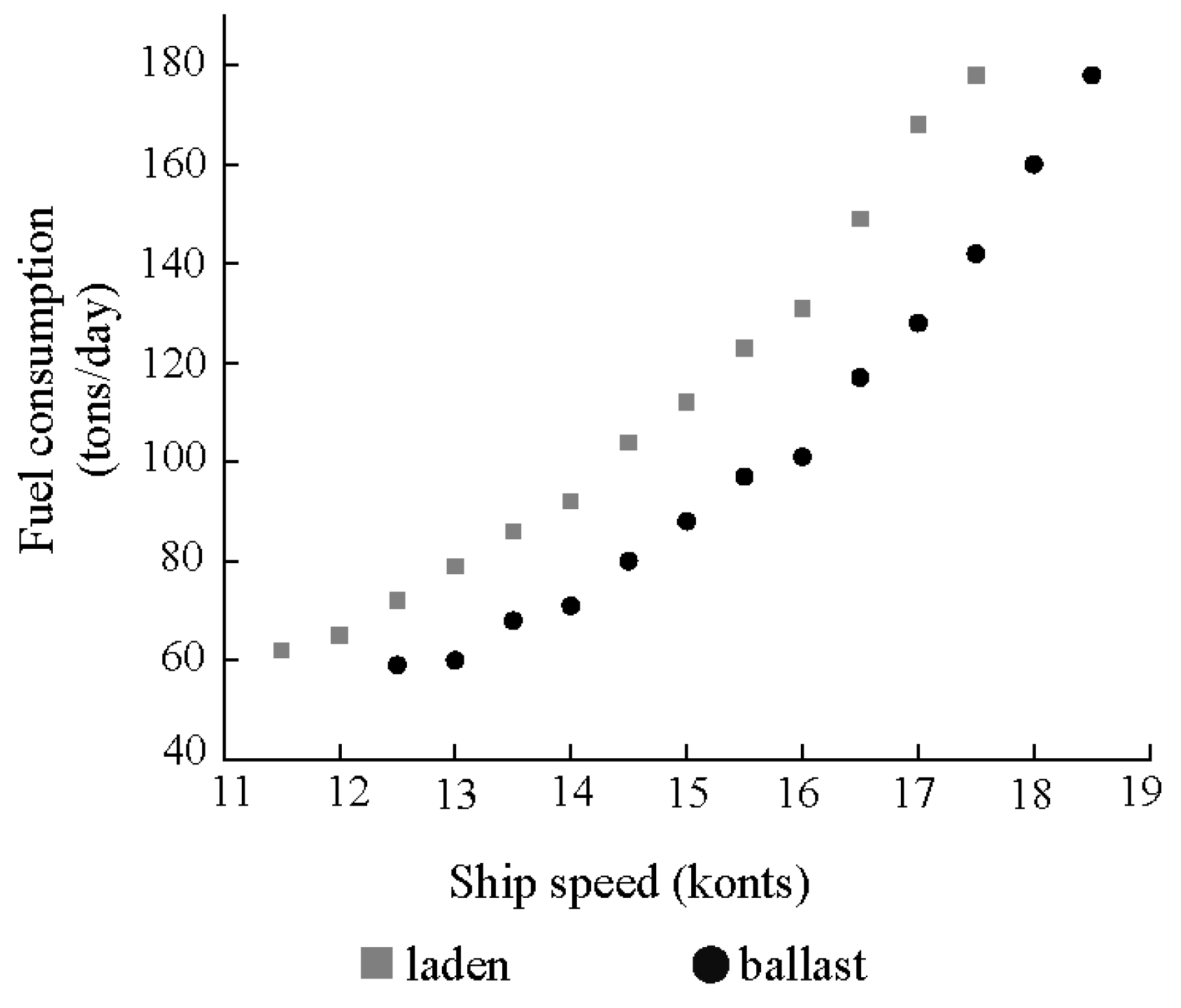
Furthermore, the payload of a ship also affects its fuel consumption and must be considered for obtaining accurate fuel cost estimates. In tankers and bulk carriers, we have a ‘binary’ situation as the ship is typically either full or empty, and the difference in fuel consumption between these two conditions can be quite substantial. Figure 2 shows the fuel consumption function for Very Large Crude Carriers under laden and ballast conditions [14], the difference between laden and ballast fuel consumption at the same speed is on the order of 25–30%. If a ship’s loading condition varies along the legs of ship routes which is typical in simultaneous pickup and delivery problem, it is crucial to consider the impact of payload on fuel consumption.
At present, in the research of ship routing and scheduling problems, there is little literature that considers the influence of ship speed and payload on fuel consumption at the same time. Psaraftis and Kontovas [5] presented a survey of speed models in maritime transportation in which ship speed is one of the decision variables and proposed a ship fuel consumption calculation model considering the ship speed and payload. Based on this, Wen et al. [15] studied the tramp ship routing and scheduling problem considering speed optimization and simultaneous pickup and delivery under time, cost and environmental constraints and developed a heuristic branch-and-price algorithm for this problem. Also based on this calculation model, Fan et al. [3] studied the tramp ship routing and scheduling problem considering carbon emissions, configuration of owner and charter ships, and the impact of sailing speed.
To sum up, when studying fuel consumption of ships, most of the existing studies assume that the fuel consumption is constant or only consider its relationship with the speed, but it is more realistic to consider the speed and payload at the same time. To this end, this paper constructs a mixed integer nonlinear programming model for the tramp ship routing and scheduling problem considering both ship speed and payload. Because the model has many constraints and contains nonlinear components, it is difficult to be solved directly, so Dantzig-Wolfe decomposition is used to obtain the set partitioning model of the problem, which implicitly handles the constraints and nonlinear components, and an improved branch-and-price algorithm is then proposed to solve this problem which can give an accurate solution in a relatively short time and help tramp ship companies to make more economic and environment-friendly routing and scheduling plans. The validity of the model and algorithm proposed in this paper is simulated and verified through numerical experiments on a large number of instances, and the influences of speed and payload on fuel consumption of ships are analyzed.

2. Mathematical Model

2.1. A Nonlinear Programming Model

This paper concerns the tramp ship routing and scheduling problem considering ship speed and payload, which requires the cargo to be transported from its pickup port to the corresponding delivery port while satisfying the time window and ship capacity constraints. The objective is to minimize the fuel consumption during the entire sailing process.
Usually, the fuel consumption per-unit time (tons/day) of the ship is a function of the speed and load of the ship. This paper adopts the fuel consumption function proposed by Psaraftis and Kontovas [6]:
f v , l = k p + v q l + W r ,
The variables v, l represent speed (knots) and payload (tons) of the ship respectively, A is the ballast weight of the ship (tons), that is the weight of the ship when is does not carry any cargo. k, p, q, r are constants, k > 0 , p 0 , q 3 . Most of the existing literatures believe that the relationship between fuel consumption and speed is cubic, that is p = 0, q = 3, this paper adopts the same setting. At a given speed, f is proportional to l i j + A 2 / 3 , that is, r = 2 / 3 [16], k is the daily fuel consumption of the ship sailing at the maximum speed and at full capacity. When calculating the fuel consumption per unit distance, it can be converted through a simple functional d = v t , where t is the sailing time of the ship.
Parameters and Variables:
  • N = 0 , 1 , , n , n + 1 , , 2 n + 1 set of ports, 0, 2 n + 1 represent the virtual origin and destination depots respectively
  • P = 1 , , n set of pickup ports
  • D = n + 1 , , 2 n set of delivery ports
  • A = i , j : i , j N , i j set of arcs
  • G = N , A a directed graph
  • K set of ships (note: a ship carries only one type of cargo)
  • Q ship capacity
  • W weight of ballast ship
  • S m set of ship optional speed, assuming that the speed set on each arc is the same, the number of speed discretization points is m , then the speed set S m = u 1 ,   , u m , for any v s   S m corresponds to the same speed range v _ , v ¯
  • i index of cargo, each cargo is associated with a pickup port i and a delivery port n + i
  • d i j distance between port i and j
  • q i demand of port i , q 0 = q 2 n + 1 = 0 , q i = q n + i i = 1 , , n
  • a i , b i time window of port i , a 0 = b 0 , a 2 n + 1 = b 2 n + 1 represent the earliest departure time at origin depot and the latest arrival time at destination depots respectively
  • s i service time at port i
Decision variables
  • x i j k equals to 1 if ship k travel from port i to port j , and 0 otherwise
  • z i j k s equals to 1 if ship k travel from port i to port j with speed v s , and 0 otherwise
  • l i k payload of ship when leaving port i
  • t i k the time for start of service for ship k at port i
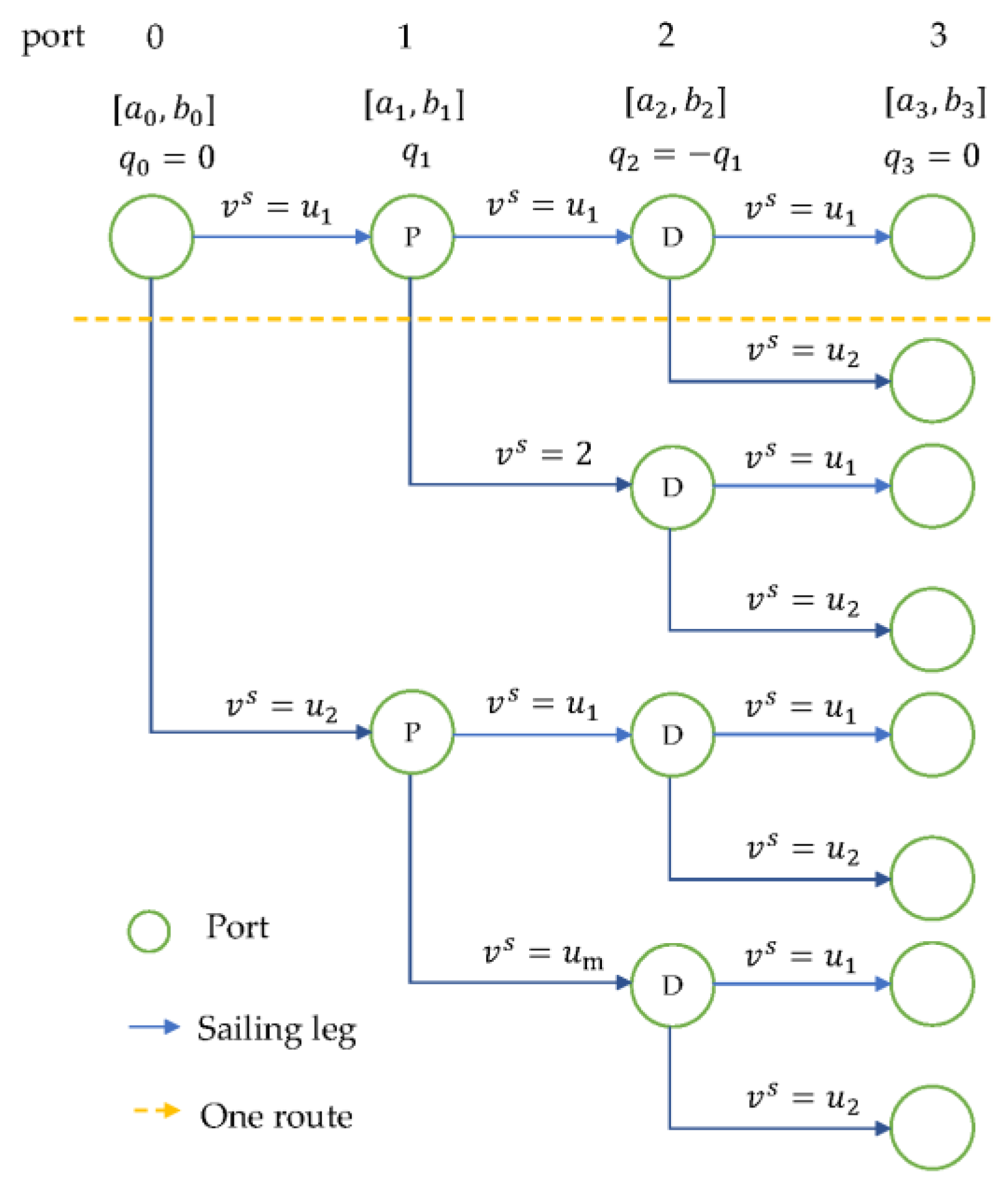
Here, we give a simple example of network with one pickup port, one delivery port and two optional speeds as shown in Figure 3. Circles in the same column represent the same port with different optional speeds when a ship travels from the previous port to this port. A ship must access the corresponding delivery port (but may not immediately) after visiting a pickup port without splitting the loads. As the number of ports and speed discretization points increase, the number of arcs in the network rises exponentially. Admittedly, not all the optional speeds satisfy the time window constraints on each port, which may reduce network complexity.
On the basis of the model of the tramp ship routing and scheduling problem proposed by Norstad et al. [11], combined with the speed discretization method proposed by Bektaş and Laporte [17] and the fuel consumption calculation model proposed by Psaraftis and Kontovas [6], a nonlinear programming model P 1 for the tramp ship routing and scheduling problem considering speed and payload is established as follow:
min k K ( i , j ) A d i j x i j k ( W k + l i k ) 2 3 ( s S ( v s ) 2 z i j k s ) ,
s.t
k ϵ K j N x i j k = 1   i   N ,
j N x i j k j N x j i k = 0   k K , j P D ,
j P 2 n + 1 x 0 j k = 1   k K ,
i D 0 x i , 2 n + 1 , k = 1   k K ,
j N x i j k j N x j , n + i , k = 0   k K , i P ,
t i k + k K s S m d i j v s z i j k s + s i t j k M 1 x i j k   k K , i , j A ,
t i k + k K s S m d i , i + n v s z i , i + n , k s + s i t i + n , k 0   k K , i P ,
a i t i k b i   k K ,   i N ,
l i k + q j l j k M 1 x i j k   k K ,   j P ,   i , j A ,
l i k q j l j + n , k M 1 x i j k   k K ,   j P ,   i , j + n A ,
j N x i j k q i l i k j N x i j k Q   k K ,   i P ,
0 l i + n , k j N x i + n , j k Q q i   k K ,   i P ,
s S z i j k s = x i j k   i , j A ,   k K ,
x i j k 0 , 1   i , j A ,   k K ,
z i j k s 0 , 1   i , j A ,   k K , s S ,
The objective function (2) minimizes fuel consumption of the ships. Constraints (3) ensures that cargoes are transported exactly once. Constraints (4)–(6) describe the network flow on a route for ship k. Coupling constraints (7) ensure that the pickup and delivery ports for a cargo i must be visited by the same ship. Precedence constraints (8) ensure that the time of starting service at a port j must be greater than or equal to the departure time from the previous port i , plus the sailing time between the nodes. Constraints (9) mean that the delivery port for a cargo must be visited after its pickup port. Constraint (10) define the time window at port i . Constraint (11) and (12) describe the quantity on board when the ship k executes pickup and delivery operation at port j respectively. Constraint (13) and (14) ensure that the capacity constraints for ship k are not violated. Constraints (15) link variables z i j k s and x i j k . Constraints (16) and (17) formulate integrality and bounds of the variables.
To verify the influence of speed and payload, we change the objective function and constraints of P 1 , and then obtain P 2 and P 3 as follow:
1.
Changing objective function (2), obtain model P 2 for tramp ship routing and scheduling problem considering ship speed.
min k K i , j A d i j x i j k ( s S v s 2 z i j k s ) ,
s.t
constraints (3)–(17).
2.
Changing objective function (2) and related constraints, obtain model P 3 for distance minimizing tramp ship routing and scheduling problem.
min k K i , j A d i j x i j k k ϵ K j N x i j k = 1     i N ,
s.t
constraints (3)–(7), (10)–(14), (16)
x i j k t i k + t t i j k + s i t j k 0     k K , i , j A ,
t i k + t t i , i + n , k + s i t i + n , k 0     k K , i P
t t i j k denote the sailing time between port i and port j with ship k at a given speed. Objective function (19) minimizes sailing distance.

2.2. Set Partitioning Formulation

To solve the problem described in Section 2.1, we applied the Dantzig—Wolfe decomposition method to model P 1 to obtain a master problem (which decides whether the routes belong to optimal solution) and a shortest path subproblem with resource constraints (which generates feasible routes), based on set partitioning [18,19]. The set partitioning model can handle a huge number of variables implicitly, effectively reduce the number of constraints, and provide a tighter linear relaxation boundary.
Let Ω denote the set of all feasible routes, i.e., the set of routes starting from a virtual origin depot, which visit some ports and arrive at the virtual destination depot, complying with constraints (3)–(17). For each route r Ω , let c r denote the cost of route r which is given by the sum of the costs of the arcs belonging to the route, and let a i r be a constant indicating the number of times port i is visited by r . Let y r be a binary variable equal to 1 if and only if route r belongs to the solution.
Through the definition above, the tramp ship routing and scheduling problem considering speed and payload can be formulated as follow:
min r Ω c r y r ,
s.t
r Ω a i r y r = 1     i P ,
y r 0 , 1     r Ω ,
Objective function (22) minimizes the cost of routes used in the solution, constraints (23) ensure each port is visited once. Constraints (24) formulate integrality and bounds of the variables.
Because of the large size of set Ω , it is difficult to solve directly. Therefor, at each branch node, a restricted master problem is obtained by giving the subset Ω ^ Ω , iteratively solve the subproblem to update routes in Ω ^ , until the subproblem no longer produces routes with negative reduced cost, and then it can be considered that we get the optimal solution of the master problem.
Restricted master problem:
m i n r Ω ^ c r y r ,
s.t
r Ω ^ a i r y r = 1     i P ,
y r 0   r Ω ^ ,
Subproblem:
min c ¯ i j x i j ,
s.t
c ¯ i j = c i j π i       |             i P , j N c i j                     |             i N \ P , j N ,
constraints (3)–(17)
and π i i N is the dual variable associated with constraints (23). Objective function (28) minimizes the reduced cost of routes used in the solution. Constraints (29) calculate the reduced cost on each arc for subproblem. In addition, we assume the number of ships equals 1 when solve the subproblem.

3. Solution Approach

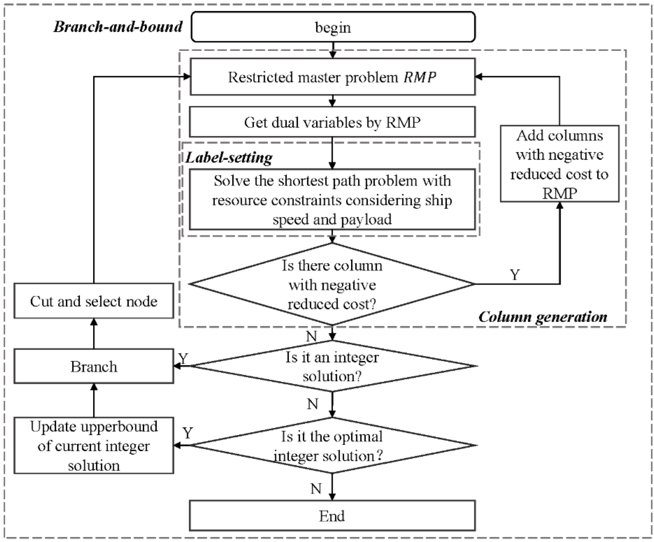
In this paper, we propose an improved branch-and-price (BP) with a tailored label-setting algorithm taking speed as a variable when constructing a route of subproblem. BP was first used by Desaulniers et al. [20] to solve the vehicle routing problem which is a combination algorithm that combines the column generation and the branch and bound. That is, solve the master problem after linear programming relaxation with the column generation to obtain the lower bound for each node of the branch and bound. For the problem studied in this paper, first, for each node of branch and bound, the dual variables are first obtained from the restricted master problem. Then the label setting algorithm is used to solve the subproblems to obtain the columns with a negative reduced cost. Finally, these columns are added to the master problem. Repeat the process above until a column with negative reduced cost cannot be generated. Then current solution is the lower bound of the node. Figure 4 presents the general process of branch-and-price.

3.1. Label Setting Algorithm

The subproblem in this study is based on the elementary shortest path problem with resource constraints considering speed, payload, time windows and simultaneous pickup and delivery problem (PDP). Ropke et al. [21] proposed a branch-price-and-cut approach for the pickup and delivery problem with time windows, in which the label setting algorithm effectively solved the elementary shortest path problem with time windows, capacity, and pickup and delivery aiming at minimizing vehicle travel distance. However, since the objective function of the problem studied in this paper is minimizing fuel consumption and take speed as a variable, which increases the complexity, and the original algorithm cannot guarantee the optimal solution of the problem. Therefor, based on the label setting algorithm proposed by Ropke et al. [21], this research gives an improved label setting algorithm to solve the subproblem.

3.1.1. Labels

For each label L , we store the following data:
  • η L : the node of the label
  • c ¯ L : the accumulated reduced cost of the route
  • l L : the payload of the ship after visiting node η L
  • t L : the arrival time at node η L
  • v L : the speed travel between the predecessor node and node η L
  • L : the set of pickup nodes which has been visited, but corresponding delivery node has not been visited
  • L : the set of unreachable nodes
The nodes in set L are divided into two categories: one is the nodes that cannot be accessed by the route due to the conflict of resource constraints such as time window constraints and capacity constraints; the other is the delivery nodes that cannot be accessed because the path has not yet visited its corresponding pickup node.
Set initial label L 0 = 0 , 0 , 0 , 0 , , , 0 . In the following, we use t L to represent the arrival time of label L , and use similar notation for the rest of the resources.

3.1.2. Label Extension

When extending a label L along an arc ( η L , j ) with speed v s S m , if both t L + t η L , j , v s b j and l L + q j Q are satisfied, and any one of the following three constraints is satisfied,
0 < j n j L ,
n < j 2 n j n L ,
n < j 2 n j n L ,
We create a new label L with following new information:
η L = j ,
c ¯ L = c ¯ L + c ¯ η L , j , v ,
t L = m a x a j , t L + t η L , j , v ,
L = L j       j N P L       j N D ,
When sailing at multiple optional speeds, the time for the ship to arrive at node j is less than a j , since sailing at a lower speed can reduce fuel consumption, it only needs to generate a new label at the lowest speed among the feasible optional speeds.

3.1.3. Dominance Criterion

To reduce the time spent searching for columns with negative reduced cost, for labels that cannot produce optimal solutions, we implement dominance criterion to remove it. Label L 1 dominates label L 2 when the following criterions are met:
η L 1 = η L 2 ,
t L 1 t L 2 ,
c ¯ ( L 1 ) c ¯ L 2 ,
L 1 = L 2 ,
L 1 L 2 ,
That is, the reduced cost of label L 1 is less than L 2 , and any feasible extension of label L 2 is also feasible for label L 1 , the dominance criterion ensures that the shortest route is preserved.
Set N = 0 , 1 , 2 , 3 , 4 , 5 , r 1 = 0 , 1 , 2 , 3 and r 2 = 0 , 3 represents the route of L 1 and L 2 respectively. Then, we can obtain L 1 = 3 , L 2 = {3}, L 1 = 5 , L 2 = 2 , 5 , which satisfies constraint (42) and constraint (43). Let σ L be the set of all feasible path from the port of label L to destination depot, then σ L 1 = 3 , 4 , 5 , σ L 2 = 3 , 4 , 5 , 3 , 4 , 1 , 2 , 5 , 3 , 1 , 2 , 4 , 5 , 3 , 1 , 4 , 2 , 5 . It is easy to see that only reserving L 1 can ensure that we get the optimal solution.

3.1.4. Acceleration Strategies

In this study, two acceleration strategies S1 and S2 are used to improve the label setting algorithm efficiency.
1.
acceleration strategies S1: set a threshold to control the number of feasible columns generated by subproblem, speeding up the convergence, and stop the search when the number of feasible columns equal to the threshold. Generally, set the threshold to twice the number of nodes. When this strategy is adopted, the number of iterations of the master problem usually increases, but the time to solve the subproblems will be greatly reduced, which can reduce the overall solution time of the branch-and-price algorithm without destroying the optimal solution of the approach.
2.
acceleration strategies S2: Feillet et al. [22] introduced the successor node set R L of the current label, R L includes nodes that satisfy resource constraints but have not been visited. If a delivery node is included in R L , it is necessary to ensure that its corresponding pickup node has been visited. In addition, since the subproblem considers speed optimization, there will be at least one arc connection between two nodes due to different speeds, and it is only necessary to ensure that sailing at any speed in the optional speed set does not violate the time window constraints.

3.1.5. Label Setting Algorithm for the Subproblem

The implementation of label setting for solving the subproblem can be described as follows:
  • Step 1: generate initial label and store it in the label set U .
  • Step 2: traversal set U , if U , generate a new label according to the label extension rules; otherwise, go to step4.
  • Step 3: based on the dominance criterion, delete dominated labels, update set U , go to step 2.
  • Step 4: detect the feasibility of the routes corresponding to the label with a negative reduced cost in the label set and add the feasible routes to the restricted master problem.
Let L i denote the set of undominated labels of node i , pseudo-code of label setting algorithm is shown in Algorithm 1.
Algorithm 1 Pseudo-Code of Label Setting Algorithm
I n p u t G = N , A
Output: P
Initialization:
U . U stores unprocessed labels
P . P stores the label corresponding to node 2n + 1 with negative reduced cost
1: U = L 0
2:while  U & nbsol < 4n do
3:   L = r e m o v e f i r s t U
4:   i = η ( L ), c i =   c L
5:  if  i = 2 n + 1 & c i < 0 do
6:    P = P L
7:   else
8:   for each feasible extension of L L do
9:   j = η ( L )
10:   if no label in L j dominates L then
11:     L j = L j L
12:     U = U L
13:    end if
14:  end for
15:end while
16:return  P

3.2. Branching Strategies

When non-integer variables exist in the solution of the master problem, we adopt branching strategy at this node. Arc branching strategy is used in this paper. First, convert route variable y r obtained by column generation into the value of the corresponding arc a i j = r Ω a i j r , where a i j r represents the value of arc i , j in route r. Then, select the arc that minimizes a i j 0.5 to branch, set a i j = 1 and a i j = 0 respectively, the optimal solution of the former must contain arc i , j , set the cost of any arc reaching i and the cost of all arcs leaving j are large enough, while the latter cannot contain arc i , j , set the cost of arc i , j large enough. Finally, recompute the solution of the new nodes.

4. Computational Experiments

In this paper, the mixed integer nonlinear programming models proposed in Section 2.2 are implemented in ILOG CPLEX 12.6.3, and the algorithm proposed in Section 3 is implemented in JAVA, and ILOG CPLEX 12.6.3 is called for solving the master problem of set partitioning model. All codes run on an Intel® Core TM i5-8500 CPU, 3.0 GHz with 8 GB of memory.

4.1. Test Instances

Since there is no benchmark for the tramp ship routing and scheduling problem considering speed and payload, and the instances in the existing literature cannot be obtained [23], this paper generates instances including 8–40 ports scales, each scale contains 9 instances. According to the ports information and actual sailing distance data provided by Brouer et al. [24], randomly select ports within the area and extract the distance between ports to generate a distance matrix. All experiments were carried out on a small bulk carrier with a ballast weight of 200 tons, capacity of 500 tons, a minimum speed of 10 knots, a maximum speed of 14 knots, and a design speed of 12 knots [25]. The port demand follows a uniform distribution with the interval (70,150) and is randomly generated. The time window is generated by a rule similar to Solomon et al. [26], the planning horizon is 60 days, the service time of ships in each port is 1 day, and the width of the time window obeys the normal distribution of μ = 3 ,   σ = 1 . Since CPLEX cannot solve model with non-integer powers in variables, in order to test the correctness and effectiveness of the BP approach. First let the parameters of formula (1) r = 1 , so that the model proposed in Section 2 can be solved in CPLEX After ensuring the correctness of the BP, let r = 2 / 3 . That is, Section 4.2 shows the results with r = 1 , Section 4.3, Section 4.4 and Section 4.5 shows the results with r = 2 / 3 .

4.2. Result of Solving P 1 by BP and CPLEX

In order to verify the correctness and effectiveness of the branch-and-price algorithm proposed in this paper to solve the tramp ship routing and scheduling problem considering speed and payload, numerical experiments are carried out with the generated instances. Based on model P 1 , BP and CPLEX are used to solve 8–40 port scale instances, respectively. BP can obtain the optimal solution for the instances of port scale of 8–40. CPLEX can obtain the optimal solution for the instances of port scale of 8–16, cannot obtain the optimal solution for the instances of port scale of 20–40 within 12 h. The results of the instances with port scales of 8–16 and 20–40 are listed in Table 1 and Table 2, respectively. The column f represents fuel consumption and column t represents computational time. It can be seen from the results that different instances under the same port scale may have huge differences in computational time, for example, when CPLEX is used to solve the instances of 16 ports scale, the minimum computational time is 776 s, while the maximum computational time exceeds 4 h. When the ports scale of the instances is larger than 16, CPLEX cannot obtain the optimal solution within the effective time. Except for instance 20–8, the optimal solution is obtained within 19 h, and the solution time of other instances is more than 24 h. Compared with CPLEX, the efficiency of the BP approach is significantly improved. When the ports scale is 40, the computational time of the BP approach is also within 1 h, the maximum is 49 min, and the average computational time is 16 min.

4.3. Analysis of the Influence of Speed and Payload

This part combines model P 1 , P 2 , P 3 , and analyzes the influence of speed and payload on the tramp ship routing and scheduling problem from five aspects, these five aspects are (a) fuel consumption FU, (b) total sailing time TT, (c) total sailing distance DI, (d) the average loading LO, (e) the number of ships used VE, as shown in Table 3. To analyze the effect of introducing speed optimization into the problem, we compare the results when speed is used as a decision variable and a fixed value, where when the speed is fixed at the design speed, the minimum speed and the maximum speed, denoted by P 3 D , P 3 M I N and P 3 M A X , respectively. The values in the table are the results of averaging 9 instances of each ports scale.
It can be seen from Table 3 that P 1 is always less than P 2 in terms of fuel consumption, which indicates that when the objective function is to minimizing fuel consumption, considering both ship speed and payload is better than considering only ship speed. Taking instances in this study as an example, the fuel consumption corresponding to P 1 is 2.42% lower on average than the fuel consumption corresponding to P 2 . However, in terms of sailing distance and time, P 2 performs better than P 1 . Combined with the average payload and the number of ships used, when both ship speed and payload are considered, due to the impact of payload on fuel consumption, ships tend to visit the corresponding delivery node as soon as possible after visiting the pickup node. As a result, individual routes are shorter, the number of routes is higher, and the average payload on a single ship is lower, making sailing distance and time longer
Regarding ship speed as decision variable can effectively reduce the fuel consumption of ships. Regardless of the design speed, the minimum speed or the maximum speed of the ship, the fuel consumption is higher than when taking ship speed as a variable, especially when sailing at maximum speed or design speed, compared with P 1 , the fuel consumption of P 3 M A X and P 3 M I N increased by 82.86% and 39.64% on average respectively. In addition, sailing at the minimum speed may violate the time window constraints and increase the number of ships used, thereby increasing the total sailing distance and fuel consumption. Based on the analysis above, considering both ship speed and payload in tramp ship routing and scheduling problem can effectively reduce fuel consumption.

4.4. Analysis of Acceleration Strategies Performance

This part tests the impact of the two acceleration strategies proposed in Section 3.1.4 on the computational time of the algorithm, as shown in Table 4. Among them, R 1 , R 2 , R 3 , R 4 respectively represent the algorithm computational time when the algorithm adopts acceleration strategies S 1 and S 2 , only S 1 , only S 2 and no acceleration strategy is adopted. Since when ports scale exceeds 24, we cannot obtain the optimal solutions of all instances within 6 h with R 2 , R 3 , R 4 , so the time in Table 4 is the average computation time of instances whose optimal solution can be obtained under each ports scale. In Table 4, the number whose optimal solution can be obtained under each ports scale is also counted, if only S 1 is adopted, when ports scale is 40, we can only obtain optimal solution of two instances. S 1 and S 2 can both improve the efficiency of the algorithm, reducing computational time by 71.48% and 79.11% respectively, adopting S 1 and S 2 at the same time reduce computational time by 91.45% on average. On average, S 2 outperforms S 1 , but there are instances where S 1 has a lower computational time.

4.5. Analysis of the Number of Speed Discretization Points

In this paper, we discretized the ship speed, the number of speed discretization points will affect the solution and computational time. We tested the effect of the number of speed discretization points on instance 1201. Let speed v 1 , , v i , , v m 1 in set of ship optional speed S m = v 1 , , v i , , v m be an arithmetic progression subject to a tolerance of t 0 , v m = v ¯ , m = v ¯ v _ t o , any speed in set S m
v i = v _ + i × t o , i = 0 , 1 , , m 1 ,
take m = 3 then S 3 = 10 , 12 , 14 , and so on.
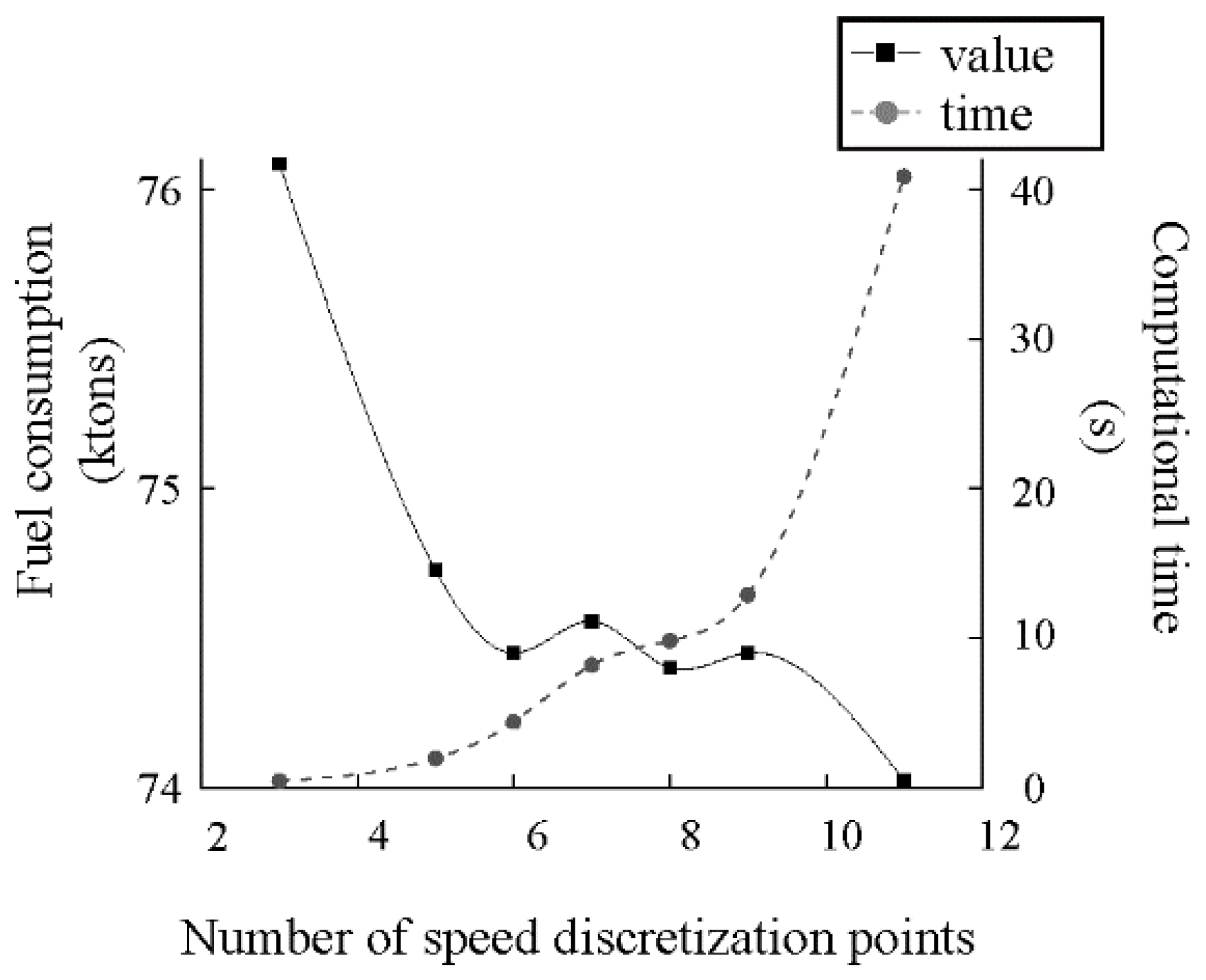
In fact, due to the non-linear relationship between fuel consumption and ship speed, as shown if Figure 1, if the time window constraint is not considered, a ship always sails at the minimum speed in the speed range. When a time window is added to each node and there will be conflicts when sailing at a small speed, in order to meet the time window constraints, the ship can only choose to sail at a higher speed. If the speed variable is continuous, the optimal speed lies between the two discrete speeds and cannot be equal to the smaller one. That is, other things being equal, the objective function value obtained with continuous speed variable is better than the value obtained with discretized speed variable. As shown in Figure 5, as the number of speed discretization points increases, the objective function value obtained by the discretized model approached optimal objective function value, but computational time increases significantly. It is worth noting that the objective function value does not decrease entirely with the number of optional speeds, e.g., in instances with 12 ports scale, when the number of optional speeds is 7, the objective function value increased compared with 6 or 9. That is caused by the different speed differences, a smaller speed difference cannot guarantee that the difference between the selectable speed and the optimal speed is closer, so a smaller speed difference may also bring about a reduction in the objective function value.

5. Conclusions

We studied the tramp ship routing and scheduling problem considering ship speed and payload, established its mixed integer non-linear programming model and set partitioning model. Based on the set partitioning model and the discretization of speed variables, an improved branch-and-price approach was designed to solve the model and verified by computational experiments. The results show that the improved BP algorithm can solve instances with 40 ports optimally within 1 h, which enables tramp ship companies to respond timely and has the potential to effectively solve larger-scale tramp ship routing and scheduling problem considering ship speed and payload. In addition, considering both ship speed and payload can greatly reduce the fuel consumption of ships by 2.42% on average compared with only considering ship speed and much higher comparing with taking speed as a constant. A reasonable number of speed discretization points can enable branch-and-price to obtain high-quality solution with a reasonable computational time. A tramp ship company can decide the number of speed discretization points according to their desired solution accuracy and computational time.
Based on the research results presented in this paper, the next stage of the research will be focused on the impact of uncertain environments such as uncertain port demand and sailing time on tramp ship routing and scheduling problem.

Author Contributions

Conceptualization, L.L. and B.J.; Data curation, L.L. and B.J.; Formal analysis, L.L., B.J. and X.F.; Funding acquisition, B.J.; Investigation, L.L. and B.J.; Methodology, L.L., B.J. and S.Z.; Project administration, B.J.; Resources, B.J.; Software, L.L.; Supervision, B.J., S.S.Y. and X.F.; Validation, L.L., B.J. and X.F.; Visualization, L.L.; Writing—original draft, L.L.; Writing—review & editing, B.J., S.S.Y., S.Z. and X.F. All authors have read and agreed to the published version of the manuscript.

Funding

This work was supported by National Natural Science Foundation of China under Grant No. 72001216, and Natural Science Foundation of Hunan Province, China under Grant No. 2020JJ5780.

Institutional Review Board Statement

Not applicable.

Informed Consent Statement

Not applicable.

Data Availability Statement

Not applicable.

Conflicts of Interest

The authors declare no conflict of interest.

References

  1. Tang, M.; Ji, B.; Fang, X.; Yu, S.S. Discretization-Strategy-Based Solution for Berth Allocation and Quay Crane Assignment Problem. J. Mar. Sci. Eng. 2022, 10, 495. [Google Scholar] [CrossRef]
  2. Christiansen, M.; Fagerholt, K.; Nygreen, B.; Ronen, D. Ship routing and scheduling in the new millennium. Eur. J. Oper. Res. 2013, 228, 467–483. [Google Scholar] [CrossRef]
  3. Fan, H.; Yu, J.; Liu, X. Tramp Ship Routing and Scheduling with Speed Optimization Considering Carbon Emissions. Sustainability 2019, 11, 6367. [Google Scholar] [CrossRef] [Green Version]
  4. IMO. Fourth IMO GHG Study 2020; International Maritime Organization (IMO): London, UK, 2020. [Google Scholar]
  5. Psaraftis, H.N.; Kontovas, C.A. Speed models for energy-efficient maritime transportation: A taxonomy and survey. Transp. Res. Part C Emerg. Technol. 2013, 26, 331–351. [Google Scholar] [CrossRef]
  6. Psaraftis, H.N.; Kontovas, C.A. Ship speed optimization: Concepts, models and combined speed-routing scenarios. Transp. Res. Part C Emerg. Technol. 2014, 44, 52–69. [Google Scholar] [CrossRef] [Green Version]
  7. Wen, M.; Røpke, S.; Petersen, H.L.; Larsen, R.; Madsen, O.B.G. Full-shipload tramp ship routing and scheduling with variable speeds. Comput. Oper. Res. 2016, 70, 1–8. [Google Scholar] [CrossRef] [Green Version]
  8. De, A.; Choudhary, A.; Tiwari, M.K. Multi objective Approach for Sustainable Ship Routing and Scheduling with Draft Restrictions. IEEE Trans. Eng. Manag. 2019, 66, 35–51. [Google Scholar] [CrossRef] [Green Version]
  9. Ma, W.; Ma, D.; Ma, Y.; Zhang, J.; Wang, D. Green maritime: A routing and speed multi-objective optimization strategy. J. Clean. Prod. 2021, 305, 127179. [Google Scholar] [CrossRef]
  10. Fagerholt, K.; Laporte, G.; Norstad, I. Reducing fuel emissions by optimizing speed on shipping routes. J. Oper. Res. Soc. 2017, 61, 523–529. [Google Scholar] [CrossRef]
  11. Norstad, I.; Fagerholt, K.; Laporte, G. Tramp ship routing and scheduling with speed optimization. Transp. Res. Part C Emerg. Technol. 2011, 19, 853–865. [Google Scholar] [CrossRef]
  12. De, A.; Mamanduru, V.K.R.; Gunasekaran, A.; Subramanian, N. Composite particle algorithm for sustainable integrated dynamic ship routing and scheduling optimization. Comput. Ind. Eng. 2016, 96, 201–215. [Google Scholar] [CrossRef]
  13. Duan, G.; Fan, T.; Chen, L.; Ma, J. Floating marine debris mitigation by vessel routing modeling and optimization considering carbon emission and travel time. Transp. Res. Part C Emerg. Technol. 2021, 133, 103449. [Google Scholar] [CrossRef]
  14. Gkonis, K.G.; Psaraftis, H.A. Modeling Tankers’ Optimal Speed and Emissions. In Proceedings of the SNAME Maritime Convention, F, 2012, Providence, RI, USA, 24 October 2012. [Google Scholar]
  15. Wen, M.; Pacino, D.; Kontovas, C.A.; Psaraftis, H.N. A multiple ship routing and speed optimization problem under time, cost and environmental objectives. Transp. Res. Part D Transp. Environ. 2017, 52, 303–321. [Google Scholar] [CrossRef]
  16. Barrass, B. Ship Design and Performance for Masters and Mates; Elsevier: Amsterdam, The Netherlands, 2004. [Google Scholar] [CrossRef]
  17. Bektaş, T.; Laporte, G. The Pollution-Routing Problem. Transp. Res. Part B Methodol. 2011, 45, 1232–1250. [Google Scholar] [CrossRef]
  18. Desaulniers, G.; Desrosiers, J.; Solomon, M.M. Column Generation; Springer Science & Business Media: Berlin/Heidelberg, Germany, 2006. [Google Scholar] [CrossRef]
  19. Lübbecke, M.E.; Desrosiers, J. Selected topics in column generation. Oper. Res. 2005, 53, 1007–1023. [Google Scholar] [CrossRef] [Green Version]
  20. Desrosiers, J.; Soumis, F.; Desrochers, M. Routing with time windows by column generation. Networks 1984, 14, 545–565. [Google Scholar] [CrossRef]
  21. Ropke, S.; Cordeau, J.F. Branch and cut and price for the pickup and delivery problem with time windows. Transp. Sci. 2009, 43, 267–286. [Google Scholar] [CrossRef] [Green Version]
  22. Feillet, D.; Dejax, P.; Gendreau, M.; Gueguen, C. An exact algorithm for the elementary shortest path problem with resource constraints: Application to some vehicle routing problems. Networks 2004, 44, 216–229. [Google Scholar] [CrossRef]
  23. Hemmati, A.; Hvattum, L.M.; Fagerholt, K.; Norstad, I. Benchmark Suite for Industrial and Tramp Ship Routing and Scheduling Problems. Inf. Syst. Oper. Res. 2016, 52, 28–38. [Google Scholar] [CrossRef] [Green Version]
  24. Brouer, B.D.; Alvarez, J.F.; Plum, C.E.M.; Pisinger, D.; Sigurd, M.M. A Base Integer Programming Model and Benchmark Suite for Liner-Shipping Network Design. Transp. Sci. 2014, 48, 281–312. [Google Scholar] [CrossRef] [Green Version]
  25. Lamb, T. Ship Design and Construction; Lamb, T., Ed.; SNAME: Alexandria, VA, USA, 2003; ISBN: 0-939773-40-6. [Google Scholar]
  26. Solomon, M.M. Algorithms for the Vehicle Routing and Scheduling Problems with Time Window Constraints. Oper. Res. 1987, 35, 254–265. [Google Scholar] [CrossRef]
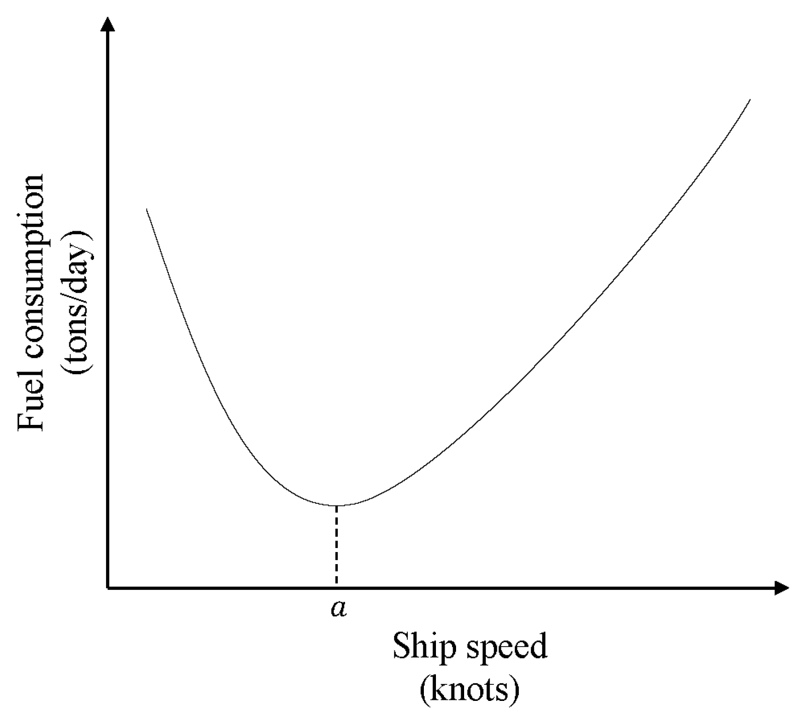
Figure 1. Qualitative graph of nonlinear relationship between carbon emission and speed.
Jmse 10 01811 g001
Figure 2. Typical fuel consumption function for a Very Large Crude Carrier.
Jmse 10 01811 g002
Figure 3. A simple example of the network.
Jmse 10 01811 g003
Figure 4. Flow chart of branch-and-price algorithm.
Jmse 10 01811 g004
Figure 5. Relationship between solution value, algorithm runtime and the number of speed discretization points.
Jmse 10 01811 g005
Table 1. Comparison results of BP and CPLEX solving P 1 for 8–16 scale instances.
InstancesCPLEXBPInstancesCPLEXBP
f (ktons)t (s)f (ktons)t (s)f (ktons)t (s)f (ktons)t (s)
080112,060712,0600.11120614,060714,0600.05
080211,1903911,1900.03120710,720310,7200.20
08039540595400.02120814,320414,3200.06
080410,6201010,6200.03120913,500313,5000.18
08059590495900.01160115,540272115,5400.97
080610,880710,8800.02160219,190565819,1900.97
080711,3801111,3800.02160322,910197522,9100.96
080812,300412,3000.01160422,550420822,5500.47
080914,230814,2300.01160526,940734326,9400.28
120114,25076814,2500.39160625,14077625,1403.98
120216,9802216,9800.12160718,77015,01118,77012.52
120320,21020420,2100.09160813,270855513,2700.64
120415,21012915,2100.11160913,71016,27613,7100.49
120516,390483616,3900.09
Table 2. Results of BP and CPLEX solving P 1 for 20–40 scale instances.
BPCPLEX BPCPLEX BPCPLEX
InstancesF
(ktons)
T
(s)
F
(ktons)
InstancesF
(ktons)
t
(s)
F
(ktons)
InstancesF
(ktons)
T
(s)
F
(ktons)
200129,860729,860280128,4313733,173360138,320203249,337
200229,7701029,770280228,430529,076360228,68012542,452
200335,0992235,099280343,8801143,880360339,0401646,897
200432,4905432,490280439,93041440,899360438,320200953,403
200523,350823,352280536,0202436,027360540,51020553,590
200618,6481518,648280630,9604431,482360634,95023739,842
200723,6465323,646280734,62032835,216360736,820440,260
200823,89057823,890280830,99010431,517360838,96032386,679
200929,2001029,202280936,1603838,913360954,5508282,466
240123,27067823,731 320139,460741,177400144,86060774,231
240225,70012325,753 320241,0902646,832400242,540102101,334
240331,9902731,992 320339,25070442,055400342,190293791,918
240420,94011620,943 320432,8302365,834400447,2202357105,974
240529,08031129,429 320541,17022745,537400533,96088365,315
240624,030524,282 320641,1203644,440400638,25069086,150
240723,6202423,736 320736,6005538,600400750,23031176,224
240823,8703124,126 320833,9904236,584400848,96011088,521
240925,5904125,805 320938,8701746,588400938,25069186,150
Table 3. Comparison results of P 1 , P 2 , P 3 .
n P 2 P 1   P 1   ( % ) P 3 D P 1   P 1   ( % ) P 3 M I N P 1   P 1   ( % ) P 3 M A X P 1   P 1   ( % )
16FU1.9239.804.5881.66
TT−9.50%−11.66%−1.47%−25.09%
DI−1.69%1.03%4.84%−7.42%
LO21.94%12.86%−6.15%45.44%
VE−11.11%−9.07%0.00%−27.04%
20FU3.96%46.41%12.29%91.20%
TT−11.05%−15.49%46.86%−23.58%
DI−0.94%−0.56%39.93%−6.72%
LO22.74%28.54%−43.02%41.10%
VE−11.67%−16.67%50.00%−24.44%
24FU2.34%43.61%4.11%92.99%
TT−11.05%−10.61%−20.68%−19.80%
DI−3.53%−3.17%−1.78%−6.12%
LO28.19%23.04%34.18%38.60%
VE−12.22%−9.44%−20.00%−16.67%
28FU2.16%39.11%3.83%84.71%
TT−12.54%−17.28%−4.83%−25.74%
DI−12.64%−12.22%−90.27%−16.77%
LO23.68%29.82%15.38%50.31%
VE−12.33%−13.07%0.00%−24.92%
32FU1.07%33.40%3.69%70.66%
TT−9.20%−4.26%16.19%−13.74%
DI−3.74%1.16%18.47%−6.98%
LO14.56%9.33%−17.46%23.42%
VE−10.69%1.01%50.00%−15.45%
36FU2.91%38.85%−0.35%80.55%
TT−10.57%−16.76%26.38%−25.37%
DI−3.06%−3.28%18.43%−9.03%
LO23.12%14.78%−11.29%42.20%
VE−10.12%−14.75%37.50%−26.06%
40FU2.58%36.31%11.39%76.59%
TT−10.65%−4.72%0.29%−22.04%
DI−3.59%−0.59%14.98%−8.45%
LO20.96%−0.32%−5.56%26.81%
VE−9.52%3.44%28.57%−19.58%
AveFU2.42%39.64%5.65%82.62%
TT−10.65%−11.54%8.96%−22.20%
DI−4.17%−2.52%0.66%−8.78%
LO22.17%16.87%−4.85%38.27%
VE−11.09%−8.37%20.87%−22.02%
Table 4. Comparison results of different acceleration strategies.
n Computational Time (ms)Number of Instances with Optimal SolutionRatio (%)
R 1 R 2 R 3 R 4 R 1 R 2 R 3 R 4 R 1 / R 4 R 2 / R 4 R 3 / R 4 R 1 / R 2 R 1 / R 3
8309944166999918.2059.8326.5630.4168.50
121211510252452799992.6733.365.578.0147.99
1623653075391313,282999917.8023.1529.4676.9060.43
2024,00554,94553,828822,03499992.926.686.5543.6944.60
24445,1511,021,615832,4716,910,95399956.4414.7812.0543.5753.47
28201,202851,233848,1632,164,77098959.2939.3239.3223.6423.72
32399,7397,110,3751,035,148-9891 - 5.6238.62
36341,6678,615,2002,555,752-9590---3.9713.37
40985,8629,327,3975,771,614-9280---10.5717.08
Ave266,6822,998,3831,233,465-----9.5529.5219.8927.3840.86
Publisher’s Note: MDPI stays neutral with regard to jurisdictional claims in published maps and institutional affiliations.