Article

The Influence of Spatial and Temporal Scales on Fisheries Modeling—An Example of Sthenoteuthis oualaniensis in the Nansha Islands, South China Sea

1
South China Sea Fisheries Research Institute, Chinese Academy of Fishery Sciences, Guangzhou 510300, China
2
College of Marine Sciences, Shanghai Ocean University, Shanghai 201306, China
3
Key Laboratory for Sustainable Utilization of Open-Sea Fishery, Ministry of Agriculture and Rural Affairs, Guangzhou 510300, China
4
Southern Marine Science and Engineering Guangdong Laboratory (Guangzhou), Guangzhou 511458, China
*
Authors to whom correspondence should be addressed.
J. Mar. Sci. Eng. 2022, 10(12), 1840; https://doi.org/10.3390/jmse10121840
Submission received: 3 November 2022 / Revised: 22 November 2022 / Accepted: 24 November 2022 / Published: 1 December 2022
(This article belongs to the Section Marine Biology)

Abstract

:
The choice of spatial and temporal scales affects the performance of fisheries models and is particularly important in exploring the relationship between resource abundance and the marine environment. Traditional fishery models are constructed at a particular scale, and the results of the study hold only at that scale. Sthenoteuthis oualaniensis is one of the main target species of large-scale light falling-net fishing in the Nansha Islands in the South China Sea. We used the S. oualaniensis fishery in the Nansha Islands as an example to compare the performance of fisheries models for 12 spatial and temporal settings and to explore the relationship between the abundance of S. oualaniensis and the marine environment in the Nansha Islands under the optimal spatial and temporal settings. The results show that the spatial and temporal scale chosen in the construction of the fishery model is not as fine as possible in generalized additive models (GAMs) for abundance index-catch per unit effort (AI-CPUE)-based scenarios, and 0.5° with the season was the best spatial and temporal setting; meanwhile, in GAMs for AI-effort-based scenarios, 0.1° with the month was the best spatial and temporal setting. The distribution of S. oualaniensis resources in the Nansha Islands was characterized by significant seasonal variation, and the monthly center of gravity had a significant negative correlation with the Niño 3.4 index and the PDO index, with correlation coefficients of 100 and 1000, respectively. It is hypothesized that Pacific Decadal Oscillation and ENSO events affect the marine environment in the South China Sea by influencing the strength of the Kuroshio force and the degree of Kuroshio curvature, which in turn affects the distribution of S. oualaniensis in the Nansha Islands. The results help us to understand the influence of spatial and temporal scales on fisheries models and the environmental factors affecting the distribution of S. oualaniensis resources in the Nansha Islands. Thus, they provide a scientific basis for the sustainable development of S. oualaniensis fisheries in this region.

1. Introduction

Sthenoteuthis oualaniensis (Ommastrephidae) is widely distributed in the Indian Ocean from 35° to 39° N and the equatorial and subtropical waters of the Pacific Ocean, with larger numbers in the South China Sea and the northwestern Indian Ocean [1,2]. S. oualaniensis is mainly divided into two populations in the Nansha Islands, a microgroup and a medium-sized group, with differences in distribution and reproduction between the two populations [3,4]. As an ecologically dependent and opportunistic species, cephalopods, represented by S. oualaniensis, are highly vulnerable to climatic anomalies in terms of resource abundance and distribution range. Anomalous climatic events can rapidly induce changes in the local environment of the fishing and spawning grounds of S. oualaniensis, leading to spatial shifts in breeding and feeding habitats and variations in abundance [5,6]. The occurrence of climate anomalies can be identified by changes in the ocean environment such as sea surface temperature, chlorophyll concentration, and thermocline depth [7]. Studies have shown that sea surface temperature anomaly (SSTA), chlorophyll-a (Chl-a), sea surface height (SSH), sea surface salinity (SSS), and mixed layer thickness (MLT) are the main environmental factors affecting a suitable S. oualaniensis habitat [8,9].
S. oualaniensis has a high economic value and an important position in the outer waters of the South China Sea. Light falling-net fishing is a new mode of fishing developed by modifying traditional lighted seine boats, where the main target catch is S. oualaniensis and a small number of phototropic fish [10]. In the spring of 2004, light falling-net fishing vessels were successful in exploratory catches of S. oualaniensis in the waters of the Central and Xisha Islands. Since then, the number of light falling-net fishing vessels heading to the outer waters of the South China Sea has increased year by year and shifted to the south-central South China Sea; in 2011, light falling-net fishing vessels began to exploit the waters of the Nansha Islands on a large scale [11,12]. Since the fishing vessel monitoring system was put into operation in Guangxi Province in 2012, all light falling-net fishing vessels in the three provinces and regions that are engaged in the fisheries development of the South China Sea have been included in real-time monitoring [13]. The productivity of light falling-net fishing vessels off the three provinces and regions near the South China Sea is characterized by a large production area, high fishing intensity in some fishing areas, and a high impact on the production of the entire South China Sea. Since the main target catch of light falling-net fishing vessels in Nansha Islands is S. oualaniensis [14], the greater the effort that is made to catch S. oualaniensis in the area where the fishing vessels gather; thus, we can use the number of light falling-net fishing vessels to characterize the amount of fishing efforts of S. oualaniensis.
Exploring the relationship between pelagic species and the marine environment, analyzing the spatial and temporal distribution patterns of their fishing grounds, and understanding their evolution is essential for the effective use and management of pelagic fisheries resources [15,16]. Previous authors have also had their preferences for choosing spatial and temporal scales when exploring the relationship between the marine environment and habitat distribution. Some scholars believe that using coarse spatial and temporal scales in fisheries modeling will reduce model performance and accuracy and may blur the relationship between the actual marine environment and species distribution [17,18]. On the other hand, some scholars believe that coarse spatial and temporal scales will bring better results of model runs and avoid the risk of overfitting to a certain extent [19,20,21]. Previous studies have rarely quantitatively compared models between scales, mostly constructed based on specific spatial and temporal (interannual, monthly, seasonal, and annual) and spatial (from 0.01° to 5°) scales. In the Southeast Pacific, researchers developed an integrated habitat suitability index model with a temporal resolution of months and a spatial resolution of 0.5° to explore the effect of climate variability on habitat suitability for jumbo flying squid, Dosidicus gigas [22]. A habitat model with a monthly temporal resolution and a spatial resolution of 0.1° was used to explore the habitat distribution of Chilean jack mackerel (Trachurus murphyi) in the Southeast Pacific [23]. These studies lacked consideration of spatial and temporal relationships and were based on data processing, model construction, and analysis of results at spatial and temporal scales selected empirically, which is not conducive to an in-depth exploration of the relationship between fishery resources and the marine environment.
The study of marine cephalopod resources by hydroacoustic methods began in the 1960s and has been reported from time to time since then [24,25,26]. It can be argued that the method of fishery acoustics is currently the most effective for assessing the abundance of S. oualaniensis [27,28]. Thus, the catch per unit effort (CPUE) of S. oualaniensis can be characterized using acoustic integral values.
Generalized additive models (GAMs) have been used in fisheries resource studies since the 1980s [29,30]. They do not require linear assumptions, are non-parametric, and provide a flexible way to explore the relationship between fisheries resources and the marine environment [31]. They can be used for different species and different sea areas, and when combined with a variety of environmental factors, they can better reveal relationships between the environment and the spatial and temporal distribution of fishery resources [32,33,34,35]. In the South China Sea, GAMs have been used to explore the relationship between the habitat and the marine environment of Auxis thazard and the spatial and temporal distribution of Decapterus maruadsi and its response to environmental change [36,37].
This study took S. oualaniensis in the Nansha Islands waters as an example and divided the vessel position monitoring system data, acoustic assessment data, and environmental data into 12 different spatiotemporal scales to explore the effects of different spatiotemporal scenarios on the GAMs of S. oualaniensis. It also identified the optimal spatial and temporal scales to explore the relationship between S. oualaniensis and the marine environment, and analyzed the spatial and temporal distribution of S. oualaniensis fishing grounds and the effects of climatic anomalies on S. oualaniensis. The results are intended to provide scale and scientific management recommendations for the development and management of pelagic fisheries in the South China Sea.

2. Materials and Methods

2.1. Fishery Data

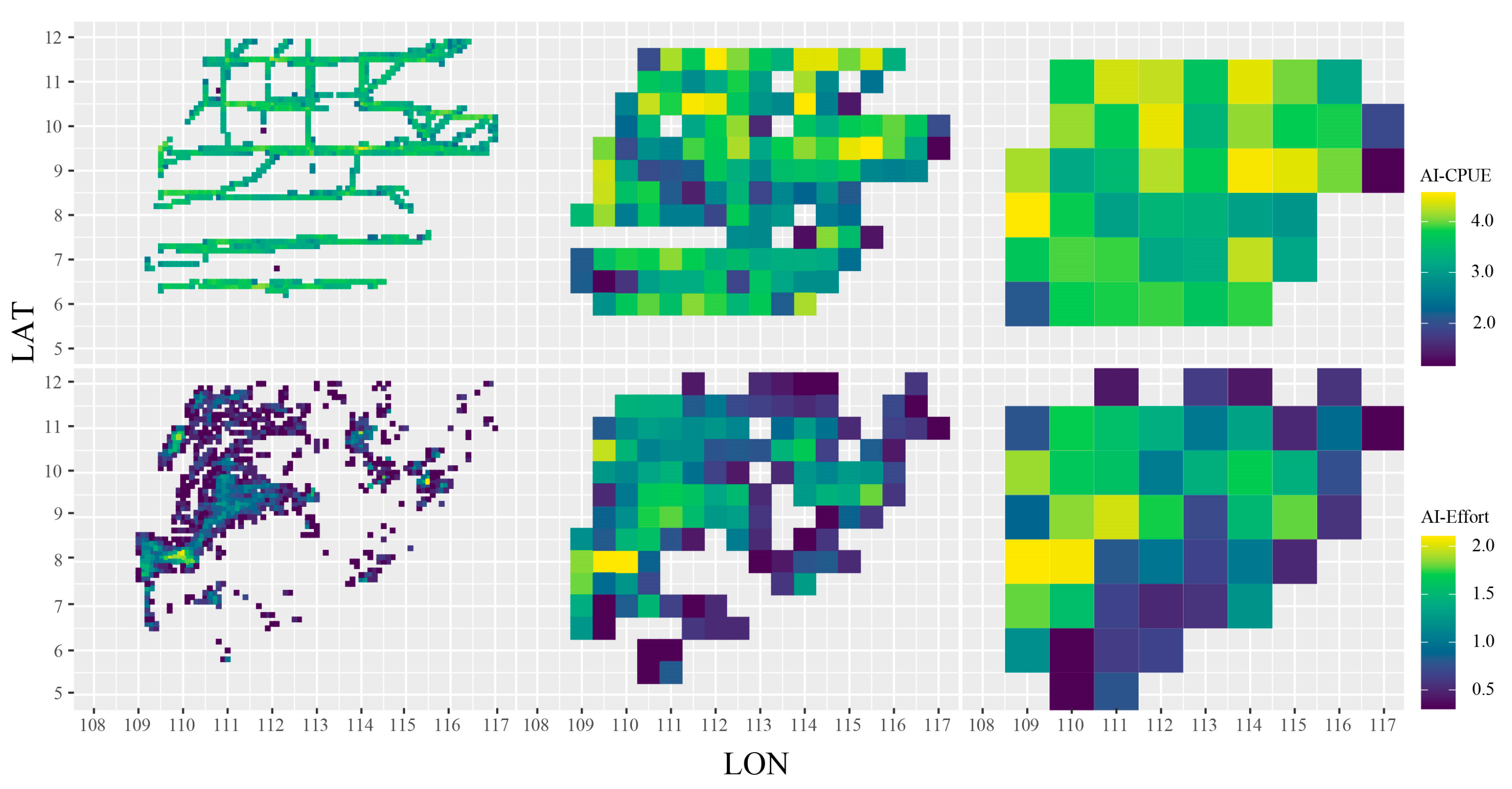
Our study area is shown in Figure 1. We selected the vessel position data of light falling-net fishing vessels south of 12° N for the period 2014–2018 and acoustic assessment data from a total of seven voyages in 2013, 2016, and 2017. An acoustic survey task was undertaken by two survey vessels with a total tonnage of 1537 Gt and 398 Gt, respectively. A count of the number of vessels appearing on each grid at each time period was performed, and the number of vessels was used to characterize the fishing effort of that grid; the higher the number of vessels, the higher the fishing effort of that grid. Therefore, the number of light falling-net fishing vessels was used to characterize the effort of the S. oualaniensis fishery in the Nansha Islands, denoted as effort-based abundance index (AI-Effort), and the acoustic integral value was used to characterize the CPUE of the S. oualaniensis fishery in the Nansha Islands, denoted as CPUE-based abundance index (AI-CPUE). The data distribution is shown in Figure 2.
The vessel position data were obtained from the database of the South China Sea Fishing Vessel Dynamic Monitoring Platform established by the South China Sea Fisheries Research Institute of the Chinese Academy of Fisheries Science. BeiDou Navigation Satellite System is China’s self-developed global satellite navigation system, consisting of a space segment, ground segment, and user segment, which can provide high-precision, highly reliable positioning, navigation, and timing services for all kinds of users around the world, all day long, with a positioning accuracy at the decimeter and centimeter levels, speed measurement accuracy of 0.2 m/s, and timing accuracy of 10 nanoseconds. The timing accuracy is 10 nanoseconds [38]. The platform relies on BeiDou Navigation Satellite System communication, with a data reception frequency of 3 min and a spatial resolution of approximately 10 m. The vessel position data include ship ID, longitude, latitude, speed, heading, and time. Owing to the substantial effect of the moon on the catch rate of S. oualaniensis, the light falling-net fishing vessels were mainly inoperative during the full moon (days 14, 15, 16 of the lunar calendar). Some vessels rested with their lights off, and some returned to port to rest and recuperate. Therefore, the vessel position data during the full moon were not indicative of the fishing effort for S. oualaniensis and were excluded [39]. Because S. oualaniensis is hardly ever found in waters less than 200 m deep, the 200 m isobath was used as a cut-off for the boat position data [39].
Acoustic assessment data were collected by Simrad EY60 and Simrad EK60 scientific fish finders, and the acoustic instrumentation was calibrated according to the internationally accepted standard target method [40]. The transducer type for both Simrad EK60 and Simrad EY60 is ES120-7C and the parameter settings are the same, the transducer gain is 27.00 dB, transmitting power is 500 W, alongship 3 dB beam width is 7.00 degrees, athwartship 3 dB beam width is 7.00 degrees, absorption coefficient is 0.045 dB·m−1, and equivalent beam angle is −21 dB. The acoustic target intensity of S. oualaniensis was analyzed at 78.1 dB, and the analysis of the acoustic data was carried out with the help of Echoview 4.9 [41]. The light falling-net fishing vessels generally switched on lights at 19:00 to lure fish, and at 21:00 the hood was snapped to end luring fish. The acoustic data between 20:00 and 21:00 were selected to analyze the echogenic intensity of S. oualaniensis. The analytical water layer was 10 to 50 m, and the analytical cell was defined as 100 ping × 5 m.

2.2. Environmental Data

The sea surface temperature anomaly (SSTA), chlorophyll-a (Chl-a), sea surface height (SSH), sea surface salinity (SSS), and mixed layer thickness (MLT) were used as environmental data in this study. The units of SSTA, Chl-a, SSS, SSH, and MLT are °C, mg-m−3, PSU, m, and m, respectively.
The SSTA were available from the National Oceanic and Atmospheric Administration (NOAA) website (https://coastwatch.pfeg.noaa.gov/data.html, accessed on 26 August 2022) and were devised from a mixture of Advanced Very High-Resolution Radiometer, Moderate-resolution Imaging Spectroradiometer, Visible Infrared Imaging Radiometer (VIIRS), and other sensors from multiple platforms such as the Aqua, Terra, and Defense Meteorological Satellite Program satellites. The data had a monthly temporal resolution and a spatial resolution of 0.01°.
Data for Chl-a were available on the NOAA website (https://coastwatch.pfeg.noaa.gov/data.html, accessed on 22 August 2022) and were obtained by the National Aeronautics and Space Administration Goddard Space Flight Center Ocean Biology Processing Group from the reanalysis of VIIRS sensor data from the Suomi-NPP satellite platform. The data had a monthly temporal resolution and a spatial resolution of 4 km.
The SSS, SSH, and MLT were provided by Copernicus Marine Environmental Monitoring Service (https://resources.marine.copernicus.eu/product-detail/GLOBAL_MULTIYEAR_PHY_001_030/INFORMATION, accessed on 27 August 2022). The data had a monthly temporal resolution and a spatial resolution of 0.083°. In the product, the MLT was defined as a depth where the density increase compared with density at 10 m depth corresponded to a temperature decrease of 0.2 °C in local surface conditions (θ10 m, S10 m, P0 = 0 db, surface pressure).
Anomalous climatic events were measured by three indicators: Niño 3.4 index, Pacific decadal oscillation (PDO) index, and southern oscillation index (SOI). The Niño 3.4 index was available from NOAA (https://origin.cpc.ncep.noaa.gov/products/analysis_monitoring/ensostuff/ONI_v5.php, accessed on 29 September 2021). The warm and cold periods were based on a threshold of +/−0.5 °C for the Oceanic Niño index (ONI) (3-month running mean of ERSST.v5 SST anomalies in the Niño 3.4 region (5° N–5° S, 120°–170° W)), based on centered 30-year base periods updated every 5 years. The PDO index was available on the Joint Institute for the Study of the Atmosphere and Ocean website (https://http://research.jisao.washington.edu/pdo/, accessed on 30 September 2021). It is defined as the leading principal component of North Pacific monthly sea surface temperature variability (poleward of 20 N for the 1900–1993 period). The SOI was available on the NOAA website (https://www.cpc.ncep.noaa.gov/data/indices/, accessed on 22 October 2021). It is defined as the difference between the standardized Tahitian barometric pressure and the standardized Darwinian barometric pressure divided by the sum of the monthly standard deviation.

2.3. Construction of the GAM

To meet the requirements of the model construction, the number of vessels and nautical area scattering coefficient (NASC) were log-transformed to satisfy a normal distribution. To avoid excessive computation and over-fitting, the linear correlation between each explanatory variable was measured according to a variance inflation factor (VIF) before the GAM was run. When VIF > 10, explanatory variables have a linear relationship with each other and should be removed from the model [42,43]. We used the R mgcv package to fit the GAM [44,45,46]. The general equation from the model can be written as:
g μ = β + f 1 x 1 + f 2 x 2 + + f i x i + ε
where g μ is the link function, which is the logarithm of catch; β is the intercept term; f is a smoothing function; i is the number of predictor variables; and ε is an error term. The GAM procedure uses smoothing splines.
The Akaike information criterion (AIC) was proposed by Akaike as a measure of the goodness of fit of a statistical model, where the smaller the AIC value, the better the model fit [47]. It is calculated as follows:
A I C = 2 k 2 l n L
where k denotes the number of independent parameters of the model and L denotes the maximum likelihood function of the model. The stability of the models was tested using 10-fold cross-validation, and the RMSE value of each model was calculated to assess the performance of the models.

2.4. Delineation of Spatial and Temporal Scales

To explore the response of the relationship between resource abundance and the marine environment to different spatial and temporal scale relationships, the current study used ArcGIS to match and reclassify the raw fisheries data with environmental data. Temporal scales included seasonal and monthly, spatial scales included 0.1° × 0.1°, 0.5° × 0.5°, and 1° × 1°, and data sources included vessel position data and acoustic assessment data. A total of 12 temporal and spatial settings were created (Table 1).

2.5. Calculation of the Center of Gravity

The weighted average of the latitude and longitude of each grid at spatial and temporal setting 7 was calculated using the distributed center of gravity method [48]. The AI-Effort or predicted values of GAM were based on spatial and temporal setting 7 as weights. The formula was as follows:
l o n ¯ = i = 1 n l o n i · D i i = 1 n D i
l a t ¯ = i = 1 n l a t i · D i i = 1 n D i
where l o n ¯ and l a t ¯ are the longitude and latitude of the center of gravity distribution, respectively; l o n i , and l a t i are the longitude and latitude of the i th grid, respectively; D i is the AI-Effort or predicted AI-Effort of the S. oualaniensis fishery at station i ; n is the number of grids.

2.6. Mapping of Fishing Grounds

The AI-CPUE was normalized using spatial and temporal setting 4, and predicted values of GAMs were based on spatial and temporal setting 4 to characterize the abundance of fishery resources. The formula was as follows:
A b u n d a n c e i = X i X m i n X m a x X m i n
where A b u n d a n c e i is the abundance value for the ith grid, X i is the AI-CPUE or predicted value for the i th grid, X m i n is the smallest AI-CPUE or predicted value for the season, and X m a x is the largest AI-CPUE or predicted value for the season. The values of A b u n d a n c e i ranged from 0–1, with values closer to 1 indicating higher abundance of S. oualaniensis resources. To aid interpretability, we plotted isoclines to signify areas of highly suitable or unsuitable habitat. We defined suitable areas (SUI-A) as those with A b u n d a n c e values ≥ 0.6, high-density areas (HIGH-A) as those with A b u n d a n c e values ≥ 0.8, and low-density areas (LOW-A) as those with A b u n d a n c e values < 0.2 [49].

2.7. Time Delay Analysis

To determine whether there is a time-lagged effect of climatic anomalous events on the monthly center of gravity distribution of the S. oualaniensis in the Nansha Islands, the spatial and temporal relationships between SOI, PDO, and Niño 3.4 and the monthly center of gravity were further evaluated using cross-correlation plots.

3. Results

3.1. Performance of Models at Different Spatial and Temporal Scales

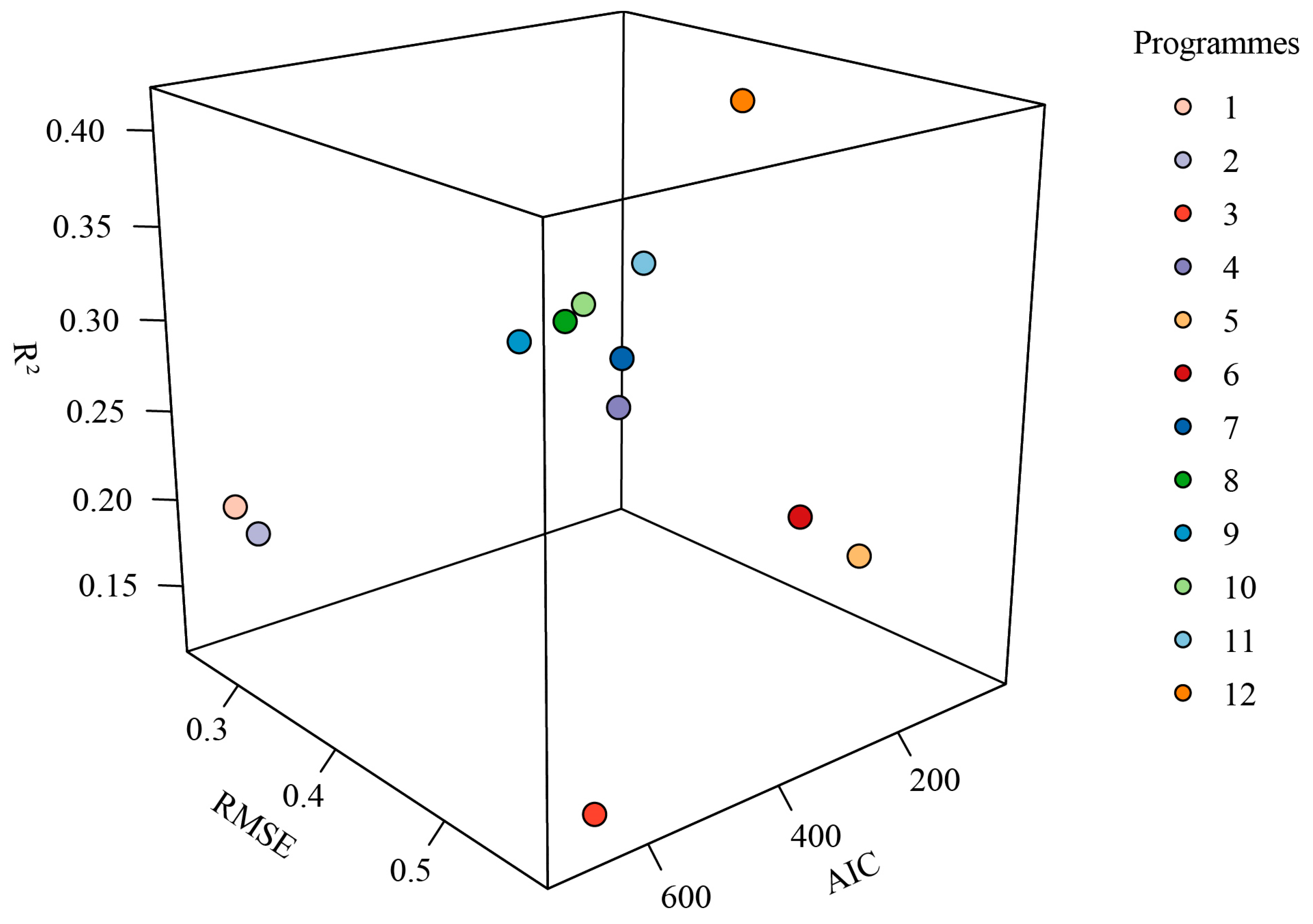
For the S. oualaniensis fishery dataset, the results of the VIF test are shown in Table 2, and the expressions and results of the GAM are shown in Table 3. The GAMs of AIs (i.e., AI-effort, AI-CPUE) with six spatial and temporal scales (i.e., 0.1° × 0.1°, 0.5° × 0.5°, 1° × 1°) were trained and tested on corresponding datasets (Table 3). For a given spatial and temporal setting, the AIC, adj-R2, and root mean squared error (RMSE) values of the models based on the two AIs differed. The RMSE generally increased with a coarsening of the spatial scale, with seasonal RMSEs generally smaller than monthly ones for scenarios based on AI-CPUE, and monthly RMSEs generally smaller than seasonal ones for scenarios based on AI-Effort. For the AI-CPUE, there was a general trend towards a progressive increase in AIC. The worst model performance occurred in setting 1, the 0.1° × 0.1° and month scenario. The best model performance occurred in setting 4, the 0.5° × 0.5° and seasonal scenario, which had the smallest RMSE and AIC. For the AI-Effort, the AIC generally tended to increase and then decrease, with the worst model performance occurring in setting 9, the 0.5° × 0.5° and seasonal scenario. The best model performance occurred in setting 7, the 0.1° × 0.1° and month scenario, which had the smallest RMSE and AIC. For the different spatial and temporal settings, the mean model adj-R2 for the AI-Effort and AI-CPUE was 0.19 and 0.3055, the mean AIC was 435.2167 and 260.5267, and the mean RMSE was 0.420667 and 0.370667, respectively. Overall, the GAMs for AI-Effort had a better performance than the GAMs for AI-CPUE at the corresponding spatial and temporal setting, with higher adj-R2, lower AIC, and RMSE (Figure 3).

3.2. Distribution of the Center of Gravity of Fishing Grounds

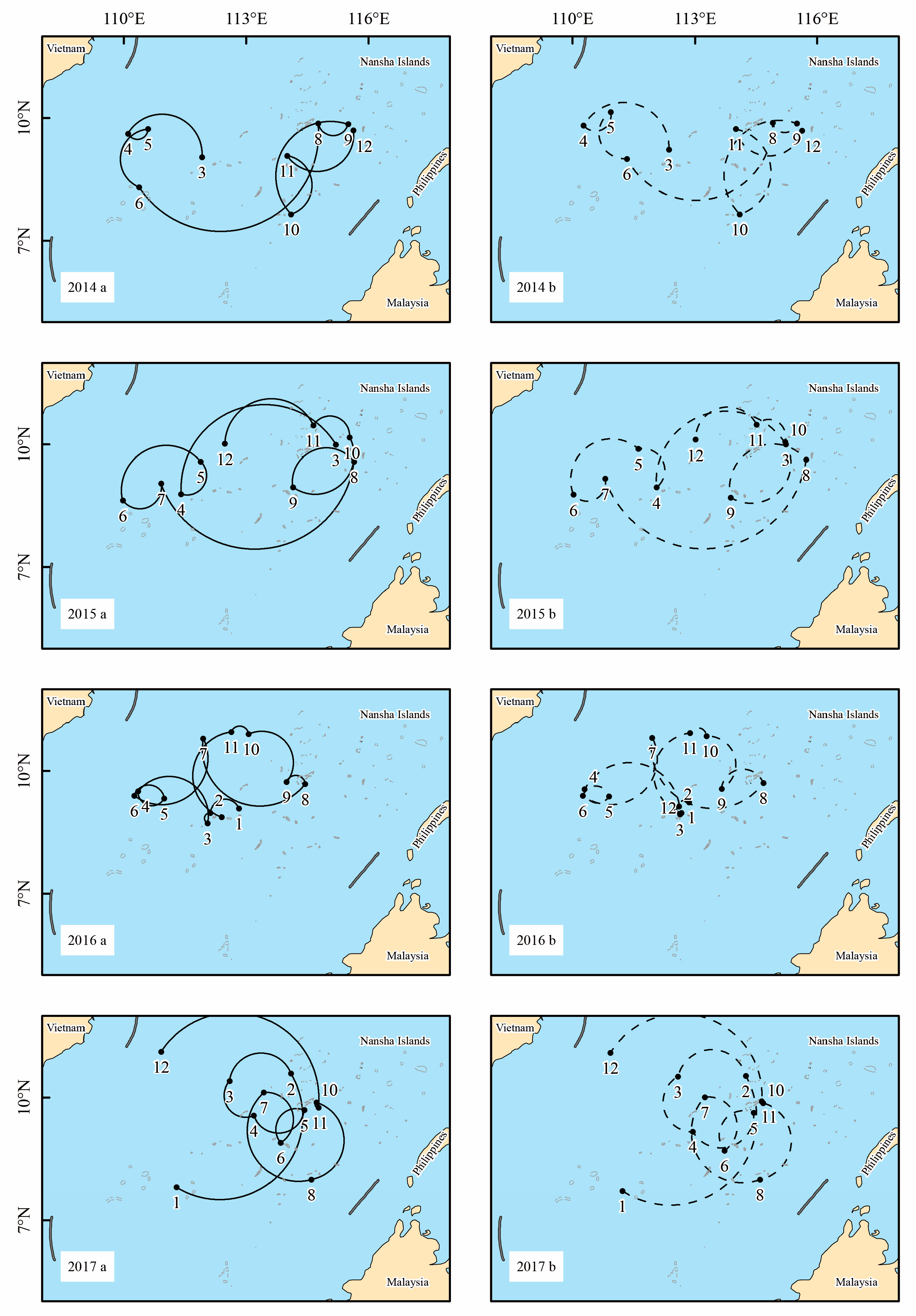
The center of gravity distribution method was used to calculate the monthly center of gravity of spatial and temporal setting 7 and the monthly center of gravity of the predicted values of the GAM constructed based on spatial and temporal setting 7, and the two were connected one by one (Figure 4). It was found that the trajectories of the actual center of gravity and the predicted center of gravity were relatively similar, with the center of gravity for each month from 2014 to 2018 mainly distributed between 8°–11° N and 109°–116° E, with large variations in the longitude direction and small variations in the latitude direction. From 2014 to 2016, the center of gravity was mainly distributed in the western part of the study area from March to July, in the eastern part of the study area from August to October, and gradually moved westwards in the central part of the study area from November to February. In 2017, the center of gravity from February to November was mainly located in the central-eastern region of the study area, with that for January and December located in the western part of the study area. In 2018, the center of gravity was located mainly in the eastern part of the study area from January to June and in the western part of the study area from July to August.
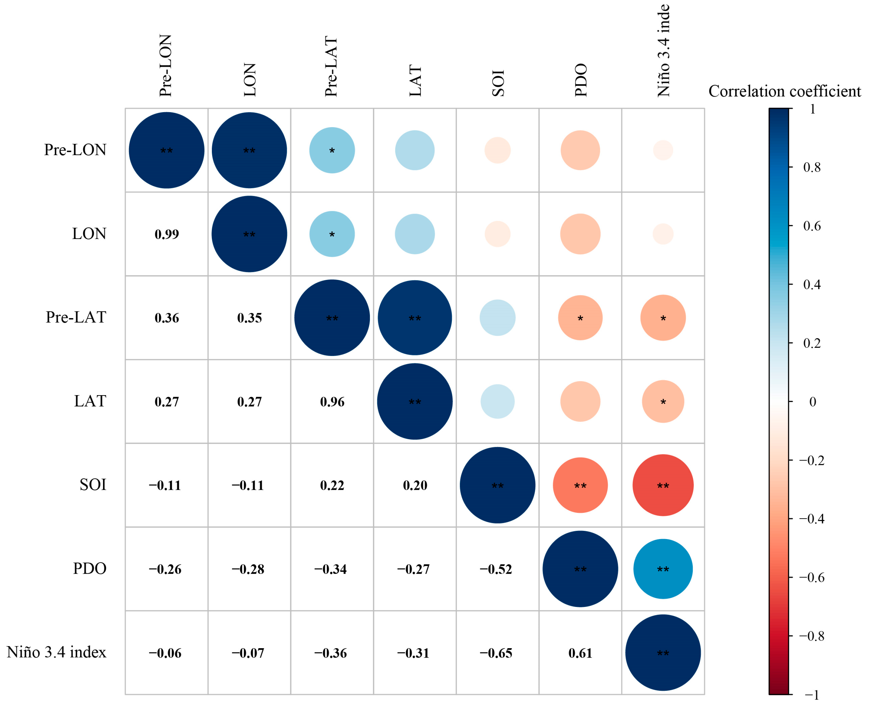
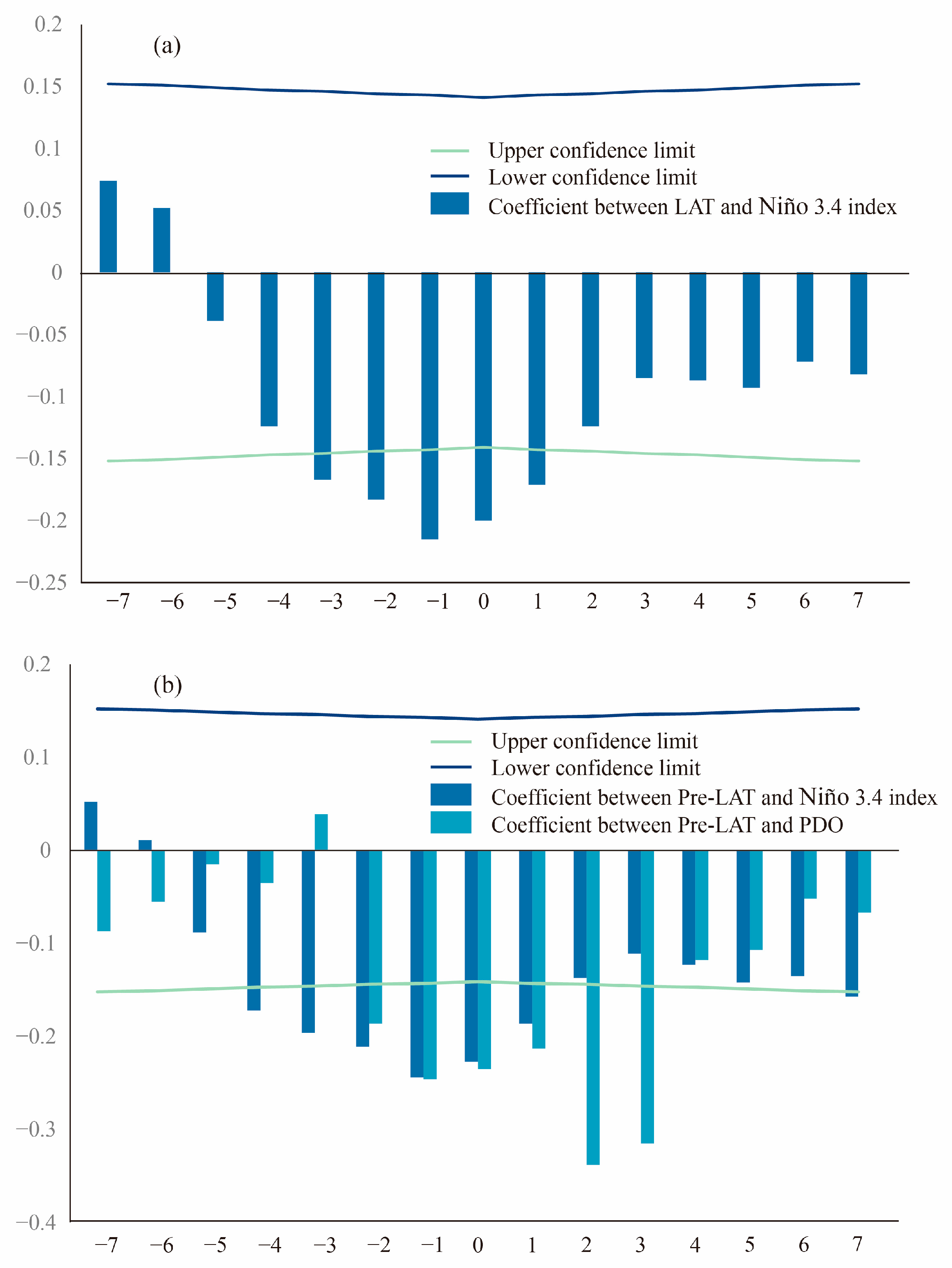
Analysis of the correlation between the center of gravity of AI-Effort and the predicted center of gravity and anomalous climatic events showed a significant negative correlation between latitude and anomalous climatic events (p < 0.05), while the correlation between longitude and anomalous climatic events was not significant (p > 0.05) (Figure 5). The correlation coefficient between the center of gravity latitude of AI-Effort and the Niño 3.4 index was −0.31, the correlation coefficient between the predicted center of gravity latitude and the PDO was −0.34, and the correlation coefficient with the Niño 3.4 index was −0.36. Cross-correlation analysis of these three sets of significant correlations was conducted to explore the lagged effects of anomalous climatic events on the distribution of the center of gravity of S. oualaniensis (Figure 6). Cross-correlation analysis showed a significant negative correlation between the center of gravity latitude of AI-Effort and the monthly Niño 3.4 index, with a lag of −3 to 1 month, and the highest correlation coefficient at a lag of one month. There was a significant negative correlation between the predicted center of gravity latitude and PDO and the monthly Niño 3.4 index, lagging −2 to 3 months, and −4 to 1 months, respectively, with the highest correlation coefficients at lags of 2 and −1 months, respectively.

3.3. Spatial and Temporal Distribution of Fishing Grounds

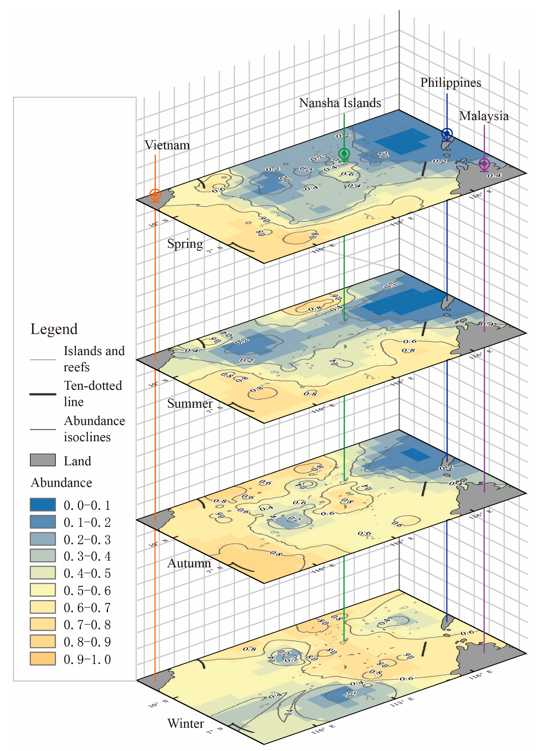
In general, the seasonal distribution of the S. oualaniensis fishing grounds obtained from the actual and predicted values was similar, and the results of the GAM at spatiotemporal setting 4 were mapped and described for the seasonal distribution of the S. oualaniensis fishing grounds (Figure 7). In spring, SUI-A was mainly located in the western part of the study area, HIGH-A was located in the northwestern and southwestern corners, while LOW-A was mainly located in the eastern part of the study area, with scattered distribution in the central-northern sea. The range of both SUI-A and HIGH-A expanded during the summer, with generally higher abundance levels across the study area. The distribution of SUI-A was mainly in the southwestern region, with SUI-A ranges contracting to the west in the north and expanding to the east in the south compared with the spring. The extent of the HIGH-A could be divided into two parts, one concentrated in the southwestern corner and the other in the central-northern part of the study area. The location of the LOW-A did not change significantly compared with spring, but the morphology was more concentrated. The overall abundance improved in the autumn. The SUI-A was mainly distributed in the central and western parts of the study area. The HIGH-A expanded in extent but could still be divided into two parts, concentrated in the southwestern corner and the central-northern sea, with a slightly dispersed morphology. The distribution of LOW-A contracted again, with no major changes in the distribution location. The overall abundance decreased in winter and SUI-A shifted to the central and eastern part of the study area, while the distribution of HIGH-A contracted noticeably and was dispersed in the central part of the study area. The distribution of LOW-A shifted to the southwestern part of the study area.

4. Discussion

4.1. Choice of Spatial and Temporal Scales

As we predicted, GAMs with different spatial and temporal settings had different performances (Figure 3 and Table 3). Owing to the environmental variations in different seas and the swimming abilities of different species, the spatial and temporal scales that should be selected for the construction of fishery models differ from sea to sea, from time to time, and from species to species [50,51]. The optimal temporal and spatial setting pairing in the AI-CPUE scenario-based GAM model of S. oualaniensis in the Nansha Islands was the season and 0.5°, whereas in the AI-Effort scenario-based GAMs, the optimal temporal and spatial scale pairing was month and 0.1°. S. oualaniensis is a pelagic cephalopod with migratory habits and its location changes over time [2]. The range of variation in the distribution of S. oualaniensis over a given period was relatively constant [52]. Over shorter periods, the spatial variation of S. oualaniensis was small and a higher resolution grid should be selected for modeling, while over longer periods, the spatial variation of S. oualaniensis was large and a lower resolution grid should be selected for modeling. For species that are strong swimmers, their locations can change rapidly and modeling should be performed at lower resolution spatial and temporal scales. It is not necessary to use particularly fine spatial and temporal scales to construct models for waters with excessive variability in the marine environment. This is because a degree of data aggregation can remove distracting information and background noise, explore the relationship between fisheries data and environmental data more clearly, reduce the possibility of overfitting, and make the model more general and transferrable [51]. Therefore, it is important to choose the time scale that matches the spatial scale to obtain a highly accurate model: a finer spatial scale needs to be matched with a shorter time scale.

4.2. Seasonal Changes in the Fishing Grounds

There are two populations of S. oualaniensis in the Nansha Islands—a medium-sized group and a microgroup—with differences in the distribution and migration of the two populations [3,4]. Figure 7 shows that the HIGH-A of S. oualaniensis in the Nansha Islands in summer and autumn can be divided into two parts, with one part located in the southwestern corner of the study area and the other in the central-northern region of the study area. The spawning grounds of the medium-sized group were located at 7° N and its adjacent sea, while the spawning grounds of the microgroup were located at 11°–13° N. The two differed in spatial distribution and did not overlap, occupying different spatial ecological niches [53]. The increasing range of HIGH-A and SUI-A in summer and autumn and the rapid decrease in winter reflects the fact that S. oualaniensis is a short-lived species that spawns and breeds in summer and autumn [4]. However, the maturation and hatching of S. oualaniensis in the micro and medium-sized colonies of SUI-A do not overlap in time, and there is a staggered peak population phenomenon, with the sexual maturation of females in the miniature colonies being slightly earlier than that of females in the medium-sized colonies [53,54]. Thus, the overall reproductive period is longer, resulting in a substantial increase in species abundance in summer and autumn, while the rapid mortality of S. oualaniensis after spawning [1,2,55] causes a significant decrease in abundance in winter. Different populations of S. oualaniensis are at different life history stages at the same time, and the distribution and migration of each population varies, with the general direction of migration being overwintering migration from shallow to deeper areas and reproductive migration from deeper to shallower areas [1,54]. As a result, winter HIGH-A and SUI-A were mainly located in the central part of the study area at deeper water depths and the northern part extending to the edges. In spring, HIGH-A and SUI-A were mainly located in the more productive eastern Vietnamese upwelling zone in the western part of the Nansha Islands waters, extending towards the shallower eastern waters at the northern and southern ends.

4.3. Monthly Change in Center of Gravity

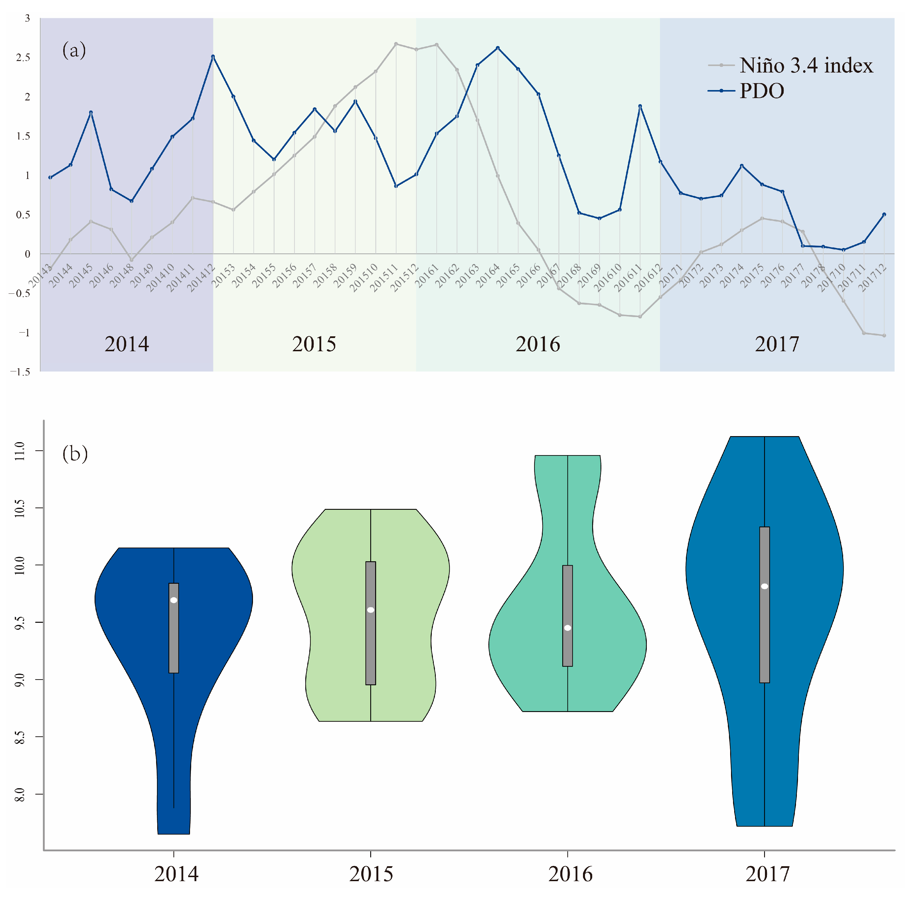
The cross-correlation analysis of the monthly distribution center of gravity of S. oualaniensis in the Nansha Islands with Niño 3.4 and PDO showed that the latitude of the monthly distribution center of gravity of the S. oualaniensis had a significant negative correlation with Niño3.4 and PDO, with a time lag of −1 and 2 months, respectively. This implies a rapid response of S. oualaniensis to large-scale changes in the marine environment. The latitudinal range of the center of gravity of S. oualaniensis in the Nansha Islands shrank and shifted northwards as large-scale anomalous climatic events intensified. At the time of the strong El Niño event in 2015, the latitudinal distribution shrank to its minimum and was evenly distributed (Figure 8). When El Niño events occur, the southeasterly trade winds weaken or shift to westerly winds, the state of high sea level in the east and low sea level in the west of the equatorial Pacific Ocean is destroyed, and the warm waters of the Western Pacific spread rapidly eastward. The warm water layer previously covering the tropical Western Pacific waters thins and the SST drops on the western side of the Pacific and rises on the eastern side [56]; thus, the center of gravity of S. oualaniensis in the Nansha Islands moves towards the southern warmer waters. S. oualaniensis have obvious vertical migration habits. In Hawaiian waters, S. oualaniensis sinks to at least 650 m water depth during the day, with water temperatures of 4–5 °C [57]. During El Niño events, the temperature of the South China Sea thermocline decreases [58], and the layer of suitable temperature for S. oualaniensis becomes shallower, which also affects the distribution of the center of gravity of S. oualaniensis in the Nansha Islands.
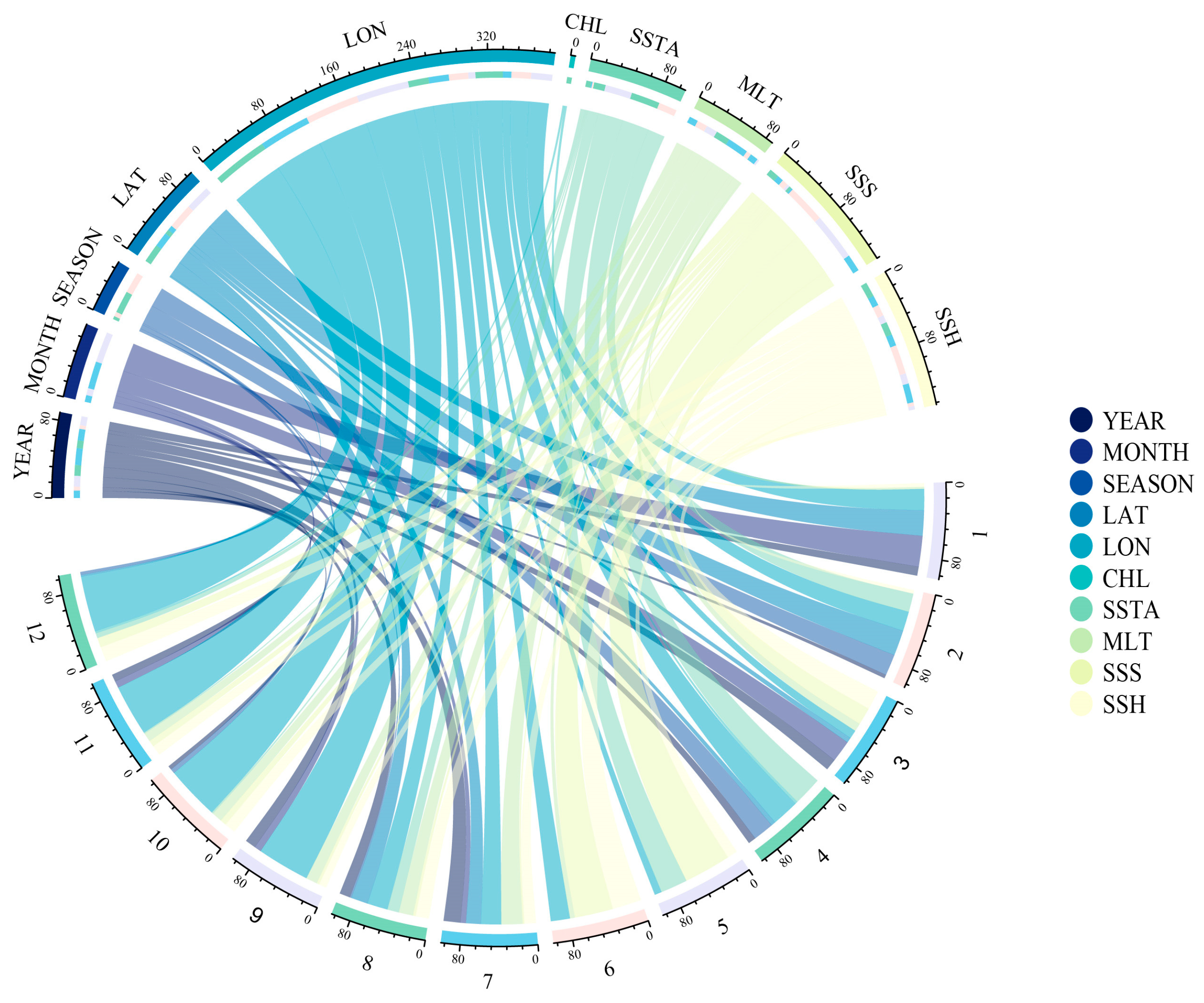
The Kuroshio Current, when flowing through the Luzon Strait, enters the South China Sea in the form of branching or flow sets, bringing warm saline water masses to the South China Sea, and influencing the thermohaline structure and circulation characteristics [59]. It has been shown that during El Niño years, westerly wind anomalies occur in the equatorial Pacific, causing the northern equatorial current divergence to shift northward, weakening the Kuroshio Current east of Luzon and enhancing the Kuroshio intrusion into the South China Sea [60,61,62,63]. When the PDO is in its warm phase, it strengthens the westerly wind anomaly in the tropical Pacific, allowing for enhanced Kuroshio incursions into the South China Sea [64]. Thus, from 2014–2017, the Kuroshio invasion of the South China Sea experienced a gradual change in strength, peaking in 2015 and then gradually declining. In contrast, the latitudinal variation in the monthly center of gravity of S. oualaniensis in the Nansha Islands underwent a process of first becoming smaller, with minimal variation in 2015, and then gradually becoming larger (Figure 8). S. oualaniensis in the South China Sea does not migrate long distances horizontally, and its passively drifting young and weakly self-swimming juveniles are mainly concentrated near islands and reefs and in waters where the Kuroshio branch intrudes into the South China Sea [65,66,67,68]. Calculating the explanatory effect of each independent variable on the response variable in the 12 constructed regression models according to the variance decomposition principle (Figure 9), it was found that the top five variables were LON, SSS, SSH, SSTA, and MLT. It can, therefore, be hypothesized that the strength of the Kuroshio intrusion into the South China Sea affects the distribution of S. oualaniensis in the Nansha Islands. The exact mechanism of influence needs further study.

4.4. Importance to Sustainable Development Goal 14

The United Nations announced the Decade of Marine Science for Sustainability in 2017 with 17 Sustainable Development Goals (SDGs). Of these, the 14th SDG, underwater life, is arguably one of the most challenging of the 17 SDGs [69]. This is because of the sheer size of the oceans (almost three-quarters of the Earth’s surface) and its direct relevance to the other SDGs [70,71,72]. More than 3 billion people get at least 20% of their daily protein from fisheries, and more than 120 million people are employed by the fisheries sector and depend on them for their livelihood [73]. Therefore, the development of sustainable fisheries is imperative and is an important component of reaching SDG 14. This study can provide advice to fisheries managers on the choice of spatial and temporal scales for fisheries modeling and help fisheries managers to grasp the distribution and changes of fisheries resources. Moreover, the investigation on the distribution range and fishery distribution of Iris squid in the Nansha Islands shows the direction for commercial fisheries and provides a reference for fishermen to conduct fishery production. Therefore, this study can contribute to SDG 14 in terms of regulating fishing activities, reducing overfishing and destructive fishing, and promoting the development of scientific management plans to restore fish stocks to at least the level that their ecological characteristics allow for producing the highest sustainable yield in the shortest possible time.

5. Conclusions

In summary, we analyzed vessel position monitoring data, acoustic assessment data, and environmental remote sensing data to explore the selection of spatial and temporal scales in constructing models for S. oualaniensis in the Nansha Islands. We reported the seasonal variation, monthly changes in the center of gravity, and response to large-scale anomalous climatic events in the fishing ground of S. oualaniensis. Comparing the 12 different spatial and temporal settings, we found that the spatial scale and the temporal scale should match when constructing the fisheries model. For example, a finer spatial scale model should have a finer temporal scale. At the same time, the rate of change in the marine environment and the swimming ability of the target species should be considered. The extent and location of the fishing grounds are profoundly influenced by favorable environmental conditions. Large-scale climatic anomalies (e.g., ENSO, PDO) had a significant negative correlation with the latitude of the monthly center of gravity of S. oualaniensis in the Nansha Islands, with a range of time lags. It was hypothesized that ENSO and PDO influenced the distribution of S. oualaniensis in the Nansha Islands by influencing the north–south movement of the north equatorial current bifurcation and the strength of the Kuroshio intrusion into the South China Sea. In future work, consideration should be given to validating vessel position data through night-time remote sensing imagery to accurately determine the operational status of commercial fishing vessels and improve the accuracy of AI-Effort modeling.

Author Contributions

Conceptualization, X.Z. and J.F.; methodology, X.Z.; software, X.Z.; validation, Y.C.; formal analysis, X.Z.; investigation, S.M. and Z.C.; resources, J.Y.; data curation, X.Z.; writing—original draft preparation, X.Z.; writing—review and editing, J.F. and Z.C.; visualization, X.Z.; supervision, Z.C.; project administration, J.F.; funding acquisition, Z.C. All authors have read and agreed to the published version of the manuscript.

Funding

This research was funded by the Key Research and Development Project of Guangdong Province (2020B1111030001), Major Projects of Basic and Applied Basic Research Programs in Guangdong Province (2019B030302004), Central Public-Interest Scientific Institution Basal Research Fund, CAFS (2020TD05), Central Public-Interest Scientific Institution Basal Research Fund, South China Sea Fisheries Research Institute, CAFS (2021SD01), and Financial Fund of the Ministry of Agriculture and Rural Affairs, P. R. of China (NFZX2021).

Data Availability Statement

The reader can ask for all the related data from the corresponding authors ([email protected]; [email protected]).

Acknowledgments

The support from the caption and crews in scientific surveys is gratefully acknowledged.

Conflicts of Interest

The authors declare no conflict of interest.

References

  1. Chen, X.J.; Liu, B.L.; Wang, Y.G. Cephalopods of the World; Ocean Press: China, Beijing, 2009. [Google Scholar]
  2. Xinjun, C.; Bilin, L.; Siquan, T.; Weiguo, Q.; Xiaohu, Z. Fishery biology of purpleback squid, Sthenoteuthis oualaniensis, in the northwest Indian Ocean. Fish. Res. 2007, 83, 98–104. [Google Scholar] [CrossRef]
  3. Zhao, C.X.; Kang, B.; He, X.B.; Yan, Y.R. Morphological, molecular, and ecological evidence in population determination and fishery management of purpleback flying squid Sthenoteuthis oualaniensis in the South China Sea. Taiwania 2021, 66, 241–250. [Google Scholar]
  4. Jiang, Y.E.; Chen, Z.; Lin, Z.; Qiu, Y.; Zhang, P.; Fang, Z. Comparison of fishery biology between medium-form and dwarf-form of Sthenoeuthis oualaniensis in South China Sea. J. Fish. China 2019, 43, 454–466. [Google Scholar]
  5. Wang, C.; Deser, C.; Yu, J.-Y.; DiNezio, P.; Clement, A. El Niño and southern oscillation (ENSO): A review. In Coral Reefs of the Eastern Tropical Pacific; Springer Science and Business Media LLC: Dordrecht, The Netherlands, 2017; pp. 85–106. [Google Scholar]
  6. Cao, J.; Chen, X.; Chen, Y. Influence of surface oceanographic variability on abundance of the western winter-spring cohort of neon flying squid Ommastrephes bartramii in the NW Pacific Ocean. Mar. Ecol. Prog. Ser. 2009, 381, 119–127. [Google Scholar] [CrossRef] [Green Version]
  7. Postuma, F.A.; Gasalla, M.A. On the relationship between squid and the environment: Artisanal jigging for Loligo plei at São Sebastião Island (24 S), southeastern Brazil. ICES J. Mar. Sci. 2010, 67, 1353–1362. [Google Scholar] [CrossRef] [Green Version]
  8. Mohamed, K.S.; Sajikumar, K.K.; Ragesh, N.; Ambrose, T.V.; Jayasankar, J.; Said Koya, K.P.; Sasikumar, G. Relating abundance of purpleback flying squid Sthenoteuthis oualaniensis (Cephalopoda: Ommastrephidae) to environmental parameters using GIS and GAM in south-eastern Arabian Sea. J. Nat. Hist. 2018, 52, 1869–1882. [Google Scholar] [CrossRef]
  9. Yu, J.; Hu, Q.; Tang, D.; Chen, P. Environmental effects on the spatiotemporal variability of purpleback flying squid in Xisha-Zhongsha waters, South China Sea. Mar. Ecol. Prog. Ser. 2019, 623, 25–37. [Google Scholar] [CrossRef]
  10. Peng, Z.; Xiaoguang, Z.; Lin, Y.; Changhan, P.E.; Xufeng, Z.H.; Sheng, Y.A.; Yongguang, T.A.; Bingzhong, Y.A.; Lei, Y.A. Analyses on fishing ground and catch composition of large-scale light falling-net fisheries in South China Sea. S. China Fish. Sci. 2013, 9, 74–79. [Google Scholar]
  11. Jiang, M.; Ma, S.; Ma, Z.; Zou, J.; Wu, S.; Lin, F.; Qin, J.; Wu, Q. Economic Benefit Analysis of Trawlers and light trap and falling net fishing vessels in South China Sea. Insights Aquacult. Biotechnol. 2018, 2, 5. [Google Scholar]
  12. Li, J.; Cai, Y.; Zhang, P.; Zhang, Q.; Jing, Z.; Wu, Q.; Qiu, Y.; Ma, S.; Chen, Z. Satellite observation of a newly developed light-fishing “hotspot” in the open South China Sea. Remote Sens. Environ. 2021, 256, 112312. [Google Scholar] [CrossRef]
  13. Zou, J.; Chen, L.; Lin, J.; Lu, Z.; Yang, B. Analysis on variation & distribution of center fishing ground for light falling-net in offshore of the South China Sea: Based on statistics of fishery surveillance to Guangxi fishing vessels. S. China Fish. Sci. 2014, 10, 78–84. [Google Scholar]
  14. Birchenough, S.E.; Cooper, P.A.; Jensen, A.C. Vessel monitoring systems as a tool for mapping fishing effort for a small inshore fishery operating within a marine protected area. Mar. Policy 2021, 124, 104325. [Google Scholar] [CrossRef]
  15. Shi, L.; Gao, Q. Policy issues on supporting China’s distant waters fisheries. Chin. Fish. Econ. 2009, 27, 69–73. [Google Scholar]
  16. Li, S.D. Policy issues on supporting China’s distant waters fisheries. Fish. Sci. 2000, 19, 42–43. [Google Scholar]
  17. Dyer, J.J.; Brewer, S.K.; Worthington, T.A.; Bergey, E.A. The influence of coarse-scale environmental features on current and predicted future distributions of narrow-range endemic crayfish populations. Freshw. Biol. 2013, 58, 1071–1088. [Google Scholar] [CrossRef]
  18. Guisan, A.; Thuiller, W.; Zimmermann, N.E. Habitat Suitability and Distribution Models: With Applications in R; Cambridge University Press: Cambridge, UK, 2017. [Google Scholar]
  19. Luoto, M.; Virkkala, R.; Heikkinen, R.K. The role of land cover in bioclimatic models depends on spatial resolution. Glob. Ecol. Biogeogr. 2007, 16, 34–42. [Google Scholar] [CrossRef]
  20. Rahbek, C.; Graves, G.R. Multiscale assessment of patterns of avian species richness. Proc. Natl. Acad. Sci. USA 2001, 98, 4534–4539. [Google Scholar] [CrossRef]
  21. Tobalske, C. Effects of Spatial Scale on the Predictive Ability of Habitat Models for the Green Woodpecker in Switzerland. In Predicting Species Occurrences: Issues of Accuracy and Scale; Scott, J.M., Heglund, P.J., Samson, F., Haufler, J., Morrison, M., Raphael, M., Wall, B., Eds.; Island Press: Covelo, CA, USA, 2002; pp. 197–204. [Google Scholar]
  22. Yu, W.; Yi, Q.; Chen, X.; Chen, Y. Modelling the effects of climate variability on habitat suitability of jumbo flying squid, Dosidicus gigas, in the Southeast Pacific Ocean off Peru. ICES J. Mar. Sci. 2016, 73, 239–249. [Google Scholar]
  23. Li, G.; Cao, J.; Zou, X.; Chen, X.; Runnebaum, J. Modeling habitat suitability index for Chilean jack mackerel (Trachurus murphyi) in the South East Pacific. Fish. Res. 2016, 178, 47–60. [Google Scholar] [CrossRef]
  24. Cabreira, A.G.; Madirolas, A.; Brunetti, N.E. Acoustic characterization of the Argentinean short-fin squid aggregations. Fish. Res. 2011, 108, 95–99. [Google Scholar] [CrossRef]
  25. Foote, K.G. Importance of the swimbladder in acoustic scattering by fish: A comparison of gadoid and mackerel target strengths. J. Acoust. Soc. Am. 1980, 67, 2084–2089. [Google Scholar] [CrossRef] [Green Version]
  26. Jefferts, K.; Burczynski, J.; Pearcy, W.G. Acoustical assessment of squid (Loligo opalescens) off the central Oregon coast. Can. J. Fish. Aquat. Sci. 1987, 44, 1261–1267. [Google Scholar] [CrossRef]
  27. Ohshimo, S. Acoustic estimation of biomass and school character of anchovy Engraulis japonicus in the East China Sea and the Yellow Sea. Fish. Sci. 1996, 62, 344–349. [Google Scholar] [CrossRef] [Green Version]
  28. Young, R.E. Cephalopods from Hawaiian waters. Fish. Bull. 1978, 76, 583. [Google Scholar]
  29. Chang, S.K.; Hoyle, S.; Liu, H.I. Catch rate standardization for yellowfin tuna (Thunnus albacares) in Taiwan’s distant-water longline fishery in the Western and Central Pacific Ocean, with consideration of target change. Fish. Res. 2011, 107, 210–220. [Google Scholar] [CrossRef]
  30. Venables, W.N.; Dichmont, C.M. GLMs, GAMs and GLMMs: An overview of theory for applications in fisheries research. Fish. Res. 2004, 70, 319–337. [Google Scholar] [CrossRef]
  31. Hastie, T.J.; Tibshirani, R.J. Generalized Additive Models. Stat. Sci. 1986, 1, 297–318. [Google Scholar] [CrossRef]
  32. Agenbag, J.J.; Richardson, A.J.; Demarcq, H.; Fréon, P.; Weeks, S.; Shillington, F.A. Estimating environmental preferences of South African pelagic fish species using catch size-and remote sensing data. Prog. Oceanogr. 2003, 59, 275–300. [Google Scholar] [CrossRef]
  33. Bacha, M.; Jeyid, M.A.; Vantrepotte, V.; Dessailly, D.; Amara, R. Environmental effects on the spatio-temporal patterns of abundance and distribution of Sardina pilchardus and sardinella off the Mauritanian coast (North-West Africa). Fish. Oceanogr. 2017, 26, 282–298. [Google Scholar] [CrossRef]
  34. Jegatheesan, J.; Zakaria, Z. Stress analysis on pressure vessel. Environ. Ecosyst. Sci. 2018, 2, 53–57. [Google Scholar] [CrossRef]
  35. Stoner, A.W.; Manderson, J.P.; Pessutti, J.P. Spatially explicit analysis of estuarine habitat for juvenile winter flounder: Combining generalized additive models and geographic information systems. Mar. Ecol. Prog. Ser. 2001, 213, 253–271. [Google Scholar] [CrossRef] [Green Version]
  36. Zhao, H.; Feng, Y.; Dong, C.; Li, Z. Spatiotemporal distribution of Decapterus maruadsi in spring and autumn in response to environmental variation in the northern South China Sea. Reg. Stud. Mar. Sci. 2021, 45, 101811. [Google Scholar] [CrossRef]
  37. Zhou, X.; Chen, Z.; Xiong, P.; Cai, Y.; Li, J.; Zhang, P.; Zhang, J.; Li, M.; Fan, J. Exploring the Spatial and Temporal Distribution of Frigate Tuna (Auxis thazard) Habitat in the South China Sea in Spring and Summer during 2015–2019 Using Fishery and Remote Sensing Data. Fishes 2022, 7, 218. [Google Scholar] [CrossRef]
  38. Yang, Y.; Mao, Y.; Sun, B. Basic performance and future developments of BeiDou global navigation satellite system. Satell. Navig. 2020, 1, 1. [Google Scholar] [CrossRef] [Green Version]
  39. Zhao, C.; Qiu, X.; He, X.; Wang, G.; Gu, Y.; Zhong, Y.; Yan, Y.; Kang, B. Relationship between lunar phase, water depth and operation time and CPUE of purpleback flying squid (Sthenoteuthis oualaniensis) in South China Sea in spring. J. Fish. China 2019, 43, 2372–2382. [Google Scholar]
  40. Simrad, E.R. Kongsberg EM Attitude 1000. Sci. Echo Sounder 2008, 212, 19–31. [Google Scholar]
  41. Zhang, J.; Chen, Z.Z.; Chen, G.B.; Zhang, P.; Qiu, Y.S.; Yao, Z. Hydroacoustic studies on the commercially important squid Sthenoteuthis oualaniensis in the South China Sea. Fish. Res. 2015, 169, 45–51. [Google Scholar] [CrossRef]
  42. Heiberger, R.M.; Heiberger, R.M.; Burt Holland, B.H. Statistical Analysis and Data Display: An Intermediate Course with Examples in R; Springer: Berlin/Heidelberg, Germany, 2015. [Google Scholar]
  43. Kutner, M.H.; Christopher, J.N.; John, N.; William, L. Applied Linear Statistical Models; McGraw-Hill Irwin: New York, NY, USA, 2005. [Google Scholar]
  44. Wood, S.N. Generalized Additive Models: An Introduction with R; Chapman and Hall/CRC: New York, NY, USA, 2006. [Google Scholar]
  45. Wood, S.N. Stable and efficient multiple smoothing parameter estimation for generalized additive models. J. Am. Stat. Assoc. 2004, 99, 673–686. [Google Scholar] [CrossRef] [Green Version]
  46. Wood, S.N. Fast stable restricted maximum likelihood and marginal likelihood estimation of semiparametric generalized linear models. J. R. Stat. Soc. Ser. B (Stat. Methodol.) 2011, 73, 3–36. [Google Scholar] [CrossRef] [Green Version]
  47. Akaike, H. Factor Analysis and AIC//Selected Papers of Hirotugu Akaike; Springer: New York, NY, USA, 1987; pp. 371–386. [Google Scholar]
  48. Garrison, L.P. Spatial Patterns in Species Composition in the Northeast United States Continental Shelf Fish Community during. In Spatial Processes and Management of Marine Populations; University of Alaska Sea Grant: Fairbanks, AK, USA, 2001; p. 513. [Google Scholar]
  49. Yu, W.; Guo, A.; Zhang, Y.; Chen, X.; Qian, W.; Li, Y. Climate-induced habitat suitability variations of chub mackerel Scomber japonicus in the East China Sea. Fish. Res. 2018, 207, 63–73. [Google Scholar] [CrossRef]
  50. Feng, Y.; Cui, L.; Chen, X.; Chen, L.; Yang, Q. Impacts of changing spatial scales on CPUE–factor relationships of Ommastrephes bartramii in the northwest Pacific. Fish. Oceanogr. 2019, 28, 143–158. [Google Scholar] [CrossRef]
  51. Núñez-Riboni, I.; Akimova, A.; Sell, A.F. Effect of data spatial scale on the performance of fish habitat models. Fish Fish. 2021, 22, 955–973. [Google Scholar] [CrossRef]
  52. Tobler, W. On the first law of geography: A reply. Ann. Assoc. Am. Geogr. 2004, 94, 304–310. [Google Scholar] [CrossRef]
  53. Xie, J.Y.; Zhang, L.Z.; Wu, W.X.; Zhou, B.H.; Chen, Q.J.; Zhao, C.X.; He, X.B.; Xv , J.; Yan, Y.R. Feeding habit and trophic niche of purpleback flying squid (Sthenoteuthis oualaniensis) in the Nansha Islands area, South China Sea. J. Fish. China 2021, 45, 1993–2002. [Google Scholar]
  54. Fan, J.; Fang, Z.; Ma, S.; Zhang, P.; Chen, Z. Age, growth, and population characteristics of Sthenoteuthis oualaniensis in the South China Sea. Reg. Stud. Mar. Sci. 2022, 55, 102517. [Google Scholar] [CrossRef]
  55. Fan, J.; Chen, Z.; Feng, X.; Yu, W. Climate-related changes in seasonal habitat pattern of Sthenoteuthis oualaniensis in the South China Sea. Ecosyst. Health Sustain. 2021, 7, 1926338. [Google Scholar] [CrossRef]
  56. McPhaden, M.J.; Zebiak, S.E.; Glantz, M.H. ENSO as an integrating concept in earth science. Science 2006, 314, 1740–1745. [Google Scholar] [CrossRef] [Green Version]
  57. Young, R.E.; Hirota, J. Review of the Ecology of Sthenoteuthis oualaniensis near the Hawaiian Archipelago. In Proceedings of the Contributed papers to International Symposium on Large Pelagic Squids, Tokyo, Japan, 18–19 July 1996. [Google Scholar]
  58. Peng, H.; Pan, A.; Zheng, Q.; Hu, J. A study of response of thermocline in the South China Sea to ENSO events. J. Oceanol. Limnol. 2018, 36, 1166–1177. [Google Scholar] [CrossRef]
  59. Shen, X.; Hu, B.; Yan, H.; Dodson, J.; Zhao, J.; Li, J.; Ding, X.; Li, Q.; Wang, X.; Xu, F. Reconstruction of Kuroshio intrusion into the south China sea over the last 40 kyr. Quat. Sci. Rev. 2022, 290, 107622. [Google Scholar] [CrossRef]
  60. Chao, S.Y.; Shaw, P.T.; Wu, S.Y. El Niño modulation of the South China sea circulation. Prog. Oceanogr. 1996, 38, 51–93. [Google Scholar] [CrossRef]
  61. Kim, Y.Y.; Qu, T.; Jensen, T.; Miyama, T.; Mitsudera, H.; Kang, H.W.; Ishida, A. Seasonal and interannual variations of the North Equatorial Current bifurcation in a high-resolution OGCM. J. Geophys. Res. Ocean. 2004, 109. [Google Scholar] [CrossRef]
  62. Qu, T.; Kim, Y.Y.; Yaremchuk, M.; Tozuka, T.; Ishida, A.; Yamagata, T. Can Luzon Strait transport play a role in conveying the impact of ENSO to the South China Sea? J. Clim. 2004, 17, 3644–3657. [Google Scholar] [CrossRef]
  63. Qu, T.; Lukas, R. The bifurcation of the North Equatorial Current in the Pacific. J. Phys. Oceanogr. 2003, 33, 5–18. [Google Scholar] [CrossRef]
  64. Wu, C.R. Interannual modulation of the Pacific Decadal Oscillation (PDO) on the low-latitude western North Pacific. Prog. Oceanogr. 2013, 110, 49–58. [Google Scholar] [CrossRef]
  65. Fan, J.T.; Chen, X.J.; Cao, J.; Tian, S.Q.; Qian, W.G.; Liu, B.L. The variation of fishing ground of Ommastrephes bartramii in the Northwest Pacific concerning with Kuroshio current. J. Shanghai Ocean. Univ. 2010, 19, 378–384. [Google Scholar]
  66. Shao, Q.Q.; Ma, W.W.; Chen, Z.Q.; You, Z.M.; Wang, W.Y. Relationship between Kuroshio meander pattern and Ommastrephes bartramii CPUE in Northwest Pacific Ocean. Oceanol. Limnol. Sin. 2005, 36, 111–122. [Google Scholar]
  67. Chen, X.J.; Xv, L.X.; Tian, S.Q. Spatial and temporal analysis of Ommastrephe bartrami resources and its fishing ground in North Pacific Ocean. J. Fish. China 2003, 27, 334–342. [Google Scholar]
  68. Tang, F.H.; Cui, X.S.; Fan, W.; Shen, X.Q.; Wu, Y.M. Study on Relationship of Neon Flying Squid Yield in North Pacific Ocean with Marine Environment by Remote Sensing. Ocean. Technol. 2011, 30, 7–12. [Google Scholar]
  69. Lee, B.X.; Kjaerulf, F.; Turner, S.; Cohen, L.; Donnelly, P.D.; Muggah, R.; Davis, R.; Realini, A.; Kieselbach, B.; MacGregor, L.S.; et al. Transforming our world: Implementing the 2030 agenda through sustainable development goal indicators. J. Public Health Policy 2016, 37, 13–31. [Google Scholar] [CrossRef]
  70. Penca, J. Mainstreaming sustainable consumption of seafood through enhanced mandatory food labeling. Front. Mar. Sci. 2020, 7, 598682. [Google Scholar] [CrossRef]
  71. Fiorentino, F.; Vitale, S. How Can We Reduce the Overexploitation of the Mediterranean Resources? Front. Mar. Sci. 2021, 8, 674633. [Google Scholar] [CrossRef]
  72. Jaiteh, V.; Peatman, T.; Lindfield, S.; Gilman, E.; Nicol, S. Bycatch estimates from a Pacific tuna longline fishery provide a baseline for understanding the long-term benefits of a large, blue water marine sanctuary. Front. Mar. Sci. 2021, 1462. [Google Scholar] [CrossRef]
  73. Molony, B.W.; Ford, A.T.; Sequeira, A.M.; Borja, A.; Zivian, A.M.; Robinson, C.; Lønborg, C.; Escobar-Briones, E.G.; Di Lorenzo, E.; Andersen, J.H.; et al. Sustainable Development Goal 14-Life Below Water: Towards a Sustainable Ocean. Front. Mar. Sci. 2022, 8, 2130. [Google Scholar] [CrossRef]
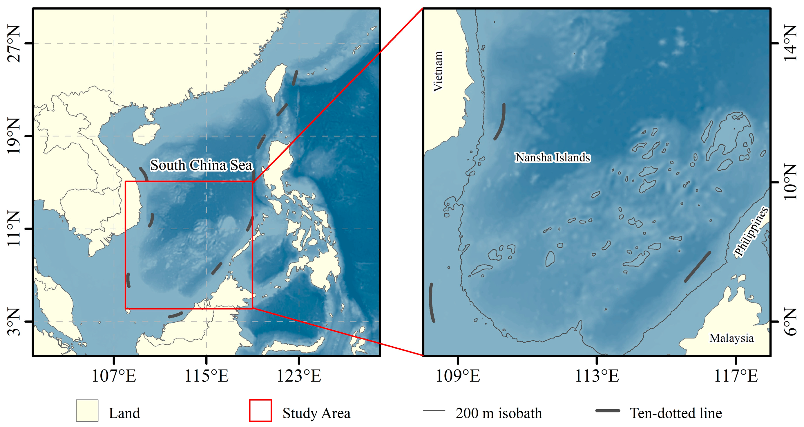
Figure 1. Study area.
Jmse 10 01840 g001
Figure 2. Distribution of AI-CPUE and AI-Effort at different spatial scales.
Jmse 10 01840 g002
Figure 3. Distribution of adj-R2, AIC, and ten-fold cross-validated RMSE on 3D scatterplots based on GAMs for 12 spatial and temporal settings.
Jmse 10 01840 g003
Figure 4. Monthly center of gravity distribution for 2014–2017 (Figure a plotted using AI-Effort projections, Figure b plotted using AI-Effort).
Jmse 10 01840 g004
Figure 5. Correlation analysis of anomalous climatic events with the latitude and longitude of the monthly center of gravity (LON refers to the longitude of the center of gravity, LAT refers to the latitude of the center of gravity, Pre-LON refers to the longitude of the predicted center of gravity, and Pre-LAT refers to the latitude of the predicted center of gravity). * p < 0.01, a statistically significant correlation. ** p < 0.001, a highly statistically significant correlation.
Jmse 10 01840 g005
Figure 6. (a) Cross-correlation coefficients between the center of gravity latitude of AI-Effort and the Niño 3.4 index. (b) Cross-correlation coefficients between the predicted center of gravity latitude and the Niño 3.4 index and the PDO.
Jmse 10 01840 g006
Figure 7. Seasonal distribution of fishing grounds of S. oualaniensis in the Nansha Islands.
Jmse 10 01840 g007
Figure 8. (a) Monthly Niño 3.4 index and PDO index for 2014–2017. (b) Latitudinal distribution range of monthly centers of gravity for 2014–2017.
Jmse 10 01840 g008
Figure 9. Extent to which each explanatory variable explains the response variable in each of the 12 spatial and temporal settings.
Jmse 10 01840 g009
Table 1. The spatial and temporal settings for GAMs.
ProgramsData ResourceSpatial ResolutionTime ResolutionNumber of Data
1AI-CPUE0.1 × 0.1month1768
2AI-CPUE0.1 × 0.1season1582
3AI-CPUE0.5 × 0.5month470
4AI-CPUE0.5 × 0.5season366
5AI-CPUE1 × 1month301
6AI-CPUE1 × 1season212
7AI-Effort0.1 × 0.1month1532
8AI-Effort0.1 × 0.1season1480
9AI-Effort0.5 × 0.5month381
10AI-Effort0.5 × 0.5season371
11AI-Effort1 × 1month188
12AI-Effort1 × 1season176
Table 2. VIF test results for each explanatory variable at different scales.
ProgramsYearSeasonMonthLonLatSSTAMLTChl-aSSSSSH
12.71——6.381.621.324.321.251.43.381.91
22.46.9——1.771.394.071.291.484.081.87
32.79——6.491.561.334.221.251.473.311.97
42.285.94——1.561.393.71.251.433.41.92
52.73——6.851.591.294.961.31.563.291.87
62.427.01——1.641.354.461.391.713.621.87
71.97——1.441.181.232.171.851.091.592.26
82.031.63——1.241.182.611.911.092.252.23
91.37——1.381.161.21.441.261.11.41.52
101.372——1.241.21.781.371.112.221.53
111.26——1.511.181.211.21.181.111.31.61
121.252.48——1.281.251.581.331.132.291.53
Table 3. Expressions, AIC, adj-R2, and 10-fold cross-validated RMSE for GAMs based on 12 spatial and temporal settings.
ProgramsData ResourceSpatial ResolutionTime ResolutionExpressionsadj-R2AICRMSEDeviance Explained
1AI-CPUE0.1 × 0.1month(lg(AI-CPUE)) ~ factor(year) + factor(month) + s(lon) + s(lat) + s(mlo) + s(ssh)0.2157420.30823
2AI-CPUE0.1 × 0.1season(lg(AI-CPUE)) ~ factor(year) + factor(season) + s(lon) + s(lat) + s(ssta) + s(ssh)0.1977130.30921.3
3AI-CPUE0.5 × 0.5month(lg(AI-CPUE)) ~ factor(year) + factor(month) + s(lon) + s(lat) + s(mlo) + s(sss) + s(ssh)0.1116040.54515.9
4AI-CPUE0.5 × 0.5season(lg(AI-CPUE)) ~ factor(year) + factor(season) + s(lon) + s(lat) + s(ssta) + s(chl)0.18535.30.25722.3
5AI-CPUE1 × 1month(lg(AI-CPUE)) ~ s(lon, k = 9) + s(ssta) + s(sss) + s(ssh)0.2182810.58529.3
6AI-CPUE1 × 1season(lg(AI-CPUE)) ~ s(lon) + s(mlo) + s(sss) + s(ssh)0.2142360.5230.7
7AI-Effort0.1 × 0.1month(lg(AI-Effort)) ~ factor(year) + factor(month) + s(lon) + s(lat) + s(mlo) + s(sss) + s(ssh) 0.213.160.24322.9
8AI-Effort0.1 × 0.1season(lg(AI-Effort)) ~ factor(year) + factor(season) + s(lon) + s(lat) + s(ssta) + s(mlo) + s(sss) + s(ssh)0.2471270.25327.2
9AI-Effort0.5 × 0.5month(lg(AI-Effort)) ~ factor(year) + factor(month) + s(lon) + s(mlo) + s(sss) + s(ssh)0.2964430.39134.4
10AI-Effort0.5 × 0.5season(lg(AI-Effort)) ~ factor(year) + factor(season) + s(lon) + s(ssta) + s(mlo) + s(sss) + s(ssh)0.3173890.41737.1
11AI-Effort1 × 1month(lg(AI-Effort)) ~ factor(year) + factor(month) + s(lon) + s(ssta) + s(mlo) + s(sss) + s(ssh)0.3413470.44540.7
12AI-Effort1 × 1season(lg(AI-Effort)) ~ factor(season) + s(lon) + s(lat) + s(ssta) + s(chl) + s(sss) + s(ssh)0.4222540.47547.6
Publisher’s Note: MDPI stays neutral with regard to jurisdictional claims in published maps and institutional affiliations.