Article

Research on PID Parameter Tuning and Optimization Based on SAC-Auto for USV Path Following

1
Key Laboratory of High Performance Ship Technology, Wuhan University of Technology, Ministry of Education, Wuhan 430070, China
2
School of Naval Architecture, Ocean and Energy Power Engineering, Wuhan University of Technology, Wuhan 430070, China
*
Author to whom correspondence should be addressed.
J. Mar. Sci. Eng. 2022, 10(12), 1847; https://doi.org/10.3390/jmse10121847
Submission received: 24 October 2022 / Revised: 15 November 2022 / Accepted: 15 November 2022 / Published: 1 December 2022
(This article belongs to the Special Issue Ship Dynamics and Hydrodynamics)

Abstract

:
Unmanned surface vessels (USVs) are required to follow a path during a task. This is essential for the USV, especially when following a curvilinear path or considering the interference of waves, and this work has been proven to be complicated. In this paper, a PID parameter tuning and optimizing method based on deep reinforcement learning were proposed to control the USV heading. Firstly, the Abkowite dynamics model with three degrees of freedom (DOF) is established. Secondly, the guidance law on the line-of-sight (LOS) method and the USV heading control system of the PID controller are designed. To satisfy the time-varying demand of PID parameters for guiding control, especially when the USV moves in waves, the soft actor–critic auto (SAC-auto) method is presented to adjust the PID parameters automatically. Thirdly, the state, action, and reward functions of the agent are designed for training and learning. Finally, numerical simulations are performed, and the results validated the feasibility and validity of the feasibility and effectiveness of the proposed method.

1. Introduction

A USV is a kind of ship which navigates on the water and is controlled by an automated algorithm or a remote device. In recent years, with the rapid development of marine science and control theory, the USV has been widely used in marine rescue and marine monitoring due to its advantages of speed and economy [1,2]. Path following is the foundation for a USV to perform tasks and is also the reflection of the intelligence of a USV.
In recent years, artificial intelligence methods, especially reinforcement learning (RL) technology, have effectively improved the accuracy of heading control for USVs. Reinforcement learning is a machine learning technique in which the agents gain knowledge about the specified scenario with training and learning from interactions with the environment directly; it can be combined with the concept of hierarchical neural networks (HNNs) in deep learning (DL) to form various types of deep reinforcement learning (DRL) methods, such as deep Q-learning network (DQN) [3], deep deterministic policy gradient (DDPG) [4], asynchronous advantage actor–critic (A3C) [5] and soft actor–critic (SAC) [6], etc. These algorithms have achieved unprecedented success in many challenging areas. In particular, reinforcement learning techniques are also used in the USV field. Gonzalez-Garcia et al. [7] proposed a USV guidance control method based on DDPG that combined sliding mode control. By training the heading command, the path following of the USV is realized. The results showed that the performance is improved, and the control stability is enhanced. Zhao et al. [8] proposed a deep Q-learning (DQL) method based on the adaptive gradient descent function to guide USV navigation. The results showed that the algorithm performs well in reducing the complexity and improving the accuracy of the path following. Wang et al. [9] proposed an optimal trajectory tracking control algorithm based on deep reinforcement learning, with which the tracking error can converge; its effectiveness and superiority are proven through simulation. The SAC algorithm is an RL algorithm proposed by Haarnoja et al., based on AC. The core idea of the algorithm is that entropy information is combined with the original reward to encourage exploration; the behavior strategy to maximize the reward with entropy is trained. The algorithm can preserve the randomness of the behavior strategy to the maximum extent and improve the agent’s ability to perceive the environment. Zheng et al. [10] proposed a linear active disturbance rejection control strategy based on the SAC algorithm, which performed the tracking on both a straight and a circular trajectory for a USV under the wave effect.
The path-following control system comprises guidance laws and controllers [11]. Line-of-sight (LOS) guidance law [12,13] has been widely used in the design of a path-following controller for USVs due to its simplicity, efficiency, and ease of implementation. The law is independent of the controller and does not depend on the mathematical model of the system. For example, in reference [14], the virtual control law that uses the tracking error is calculated to design the guidance law; in contrast, in reference [15], the visual angle of the desired path is calculated for the USV heading controller. The path-following controller can be designed with self-adaption [16,17], backstepping [18,19], sliding mode [20,21], and other control methods. However, the robustness of adaptive control methods needs to be improved. The backstepping algorithm is highly dependent on the model and needs accurate model parameters. Although sliding mode control does not require a high-accuracy model, its chattering problem is difficult to eliminate [22]. Moreover, due to the high cost of the experiment, the difficulty of adjusting the control parameters, the nonlinearity of the motion model, and the uncertainty of the environment, it is difficult to guarantee the stability of the system. Therefore, it is difficult for these control algorithms to show their advantages in practical applications.
Therefore, it is significant to propose an adaptive control method with a simple system, good robustness, and low requirement on model accuracy. PID control is widely used in a ship’s heading control. Miao et al. [23] designed a self-adapting expert S-PID controller for a mini-USV to perform heading control and verified the effectiveness and reliability of the designed motion control system through experiments. Based on the LOS guidance law, Zhu et al. [24] conducted a simulation analysis on three control algorithms, incremental PID, fuzzy PID, and variable-length-ratio-fuzzy PD, the results showed that the third has more anti-interference advantages than the other two. Fan et al. [25] designed a track control algorithm combining LOS and fuzzy adaptive PID and conducted a real boat test. The results show that the algorithm reduces the influence of time-varying drift angle on track control, however, some steering overshoot and position deviation still emerged at the corner of the path.
At present, the existing algorithms are not practical in automatically optimizing the PID parameters, and little research has been done on the application of the RL method to the heading control of USVs. For this reason, a PID parameter optimization method based on the SAC algorithm for USVs is proposed to achieve adaptive heading control. The remainder of this paper is organized as follows. In Section 2, the USV kinematic model based on Abkowite is introduced and the path-following guidance system is designed. Then the PID parameter optimization algorithm based on SAC is proposed. In Section 3, the simulation training process and the simulation results under three different working conditions are performed to verify the feasibility and effectiveness of the proposed algorithm. Finally, the concluding remarks are provided in Section 4.

2. The Design of the DRL

In this section, the overall design diagram for the proposed system is presented, and, to solve the tedious process of PID parameter tuning, an adaptive SAC-PID control method is introduced to solve the mechanical tuning problem of PID parameters. The overall flow diagram of the proposed method is given in Figure 1.
As shown in Figure 1, the Abkowitz holistic model is established, and considering the integral saturation condition of the PID controller, the control system is based on the LOS guidance and the PD controller is designed to control the USV heading. To obtain reasonable PD parameters, a neural network based on the SAC algorithm is established, and the agent is trained to interact with the abovementioned control system. The final network is used for the experimental simulation in which the required control parameters are inputted for the control parameters by online transmission.

2.1. Dynamic Model of USV

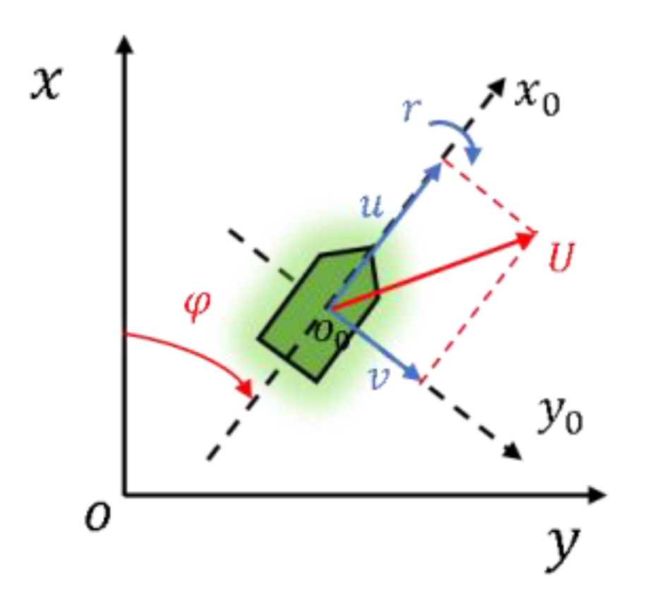
Since the USV is a kind of ship that navigates on water, a hydrodynamic model with three degrees of freedom can be used to describe the relationship between the USV’s motion state and the power, external force, fluid force, and corresponding torque on the USV in the local coordinate system of the USV. After ignoring the pitch, roll, and heave of the USV, the two-dimensional coordinate description of ship motion is shown in Figure 2, where o x y is the global coordinate system (Earth coordinate system), and o 0 x 0 y 0 is the local coordinate system of the USV.
The motion equation of the USV with three degrees of freedom can be described by the following equation:
{ X = m ( u ˙ r v x G r 2 ) Y = m ( v ˙ + r u + x G r ˙ ) N = I z r ˙ + m x G ( v ˙ + r u )
where m is the total weight of the USV, x G is the longitudinal coordinate of the center of gravity, and I z is the moment of inertia of the vertical axis over the center of gravity of the USV. X ,   Y , and N are the hydrodynamic and torque components of the USV on the 3-DOF of the three motion directions of u ,   v , and r , respectively.
The integral-type Abkowitz model refers to the motion model proposed by Abkowitz, which takes the ship as an entirety under force to process the mechanical analysis. In theory, the hydrodynamic derivative of the infinite order derived from the Taylor expansion equals the real value. Still, a large amount of research shows that the accuracy is satisfied for engineering applications when the hydrodynamic is derived from the third derivative [26,27]. The third-order Taylor series expansion model is shown in Equation (2). Δ u represents the difference between the current speed and the designed speed, which can be described as Equation (3).
{ m u ˙ r v x G r 2 = X u Δ u + X u u ( Δ u ) 2 + X u u u ( Δ u ) 3 + X u ˙ u ˙ + X v v v 2 + X r r r 2 + X v r v r + X δ δ δ 2 + X v δ v δ + X r δ r δ m v ˙ + r u + x G r ˙ = Y v v + Y v v v v 3 + Y v ˙ v ˙ + Y r r + Y r r r r 3 + Y r ˙ r ˙ + Y v r r v r 2 + Y v v r v 2 r + Y δ δ + Y δ δ δ δ 3 + Y u δ u δ + Y v δ δ v δ 2 + Y v v δ v 2 δ + Y r δ δ r δ 2 + Y r r δ r 2 δ I z r ˙ + m x G ( v ˙ + r u ) = N v v + N v v v v 3 + N v ˙ v ˙ + N r r + N r r r r 3 + N r ˙ r ˙ + N v r r v r 2 + N δ δ + N δ δ δ δ 3 + N u δ u δ + N v δ δ v δ 2 + N v v δ v 2 δ + N r δ δ r δ 2 + N r r δ r 2 δ
Δ u = u u 0
Move all terms that are proportional to translational accelerations u ˙ ,   v ˙ , and r ˙ in Equation (2) to the left of the equation, while the inertial force, the lift force, and the drag force of the fluid on the hull have been moved to the right of the equation. Then the Abkowitz mathematical model of ship motion can be given as shown in Equation (4). The USV model parameters are shown in Table 1. Table 2 contains the hydrodynamic coefficients.
{ ( m X u ˙ ) u ˙ = F X ( u , v , r , δ ) ( m Y v ˙ ) v ˙ + ( m x G Y r ˙ ) = F Y ( u , v , r , δ ) ( m x G N v ˙ ) v ˙ + ( I z N r ˙ ) r ˙ = F N ( u , v , r , δ )
where X u ˙ , Y v ˙ , Y r ˙ , N v ˙ ,   and   N r ˙ are the hydrodynamic derivatives.

2.2. Path Following

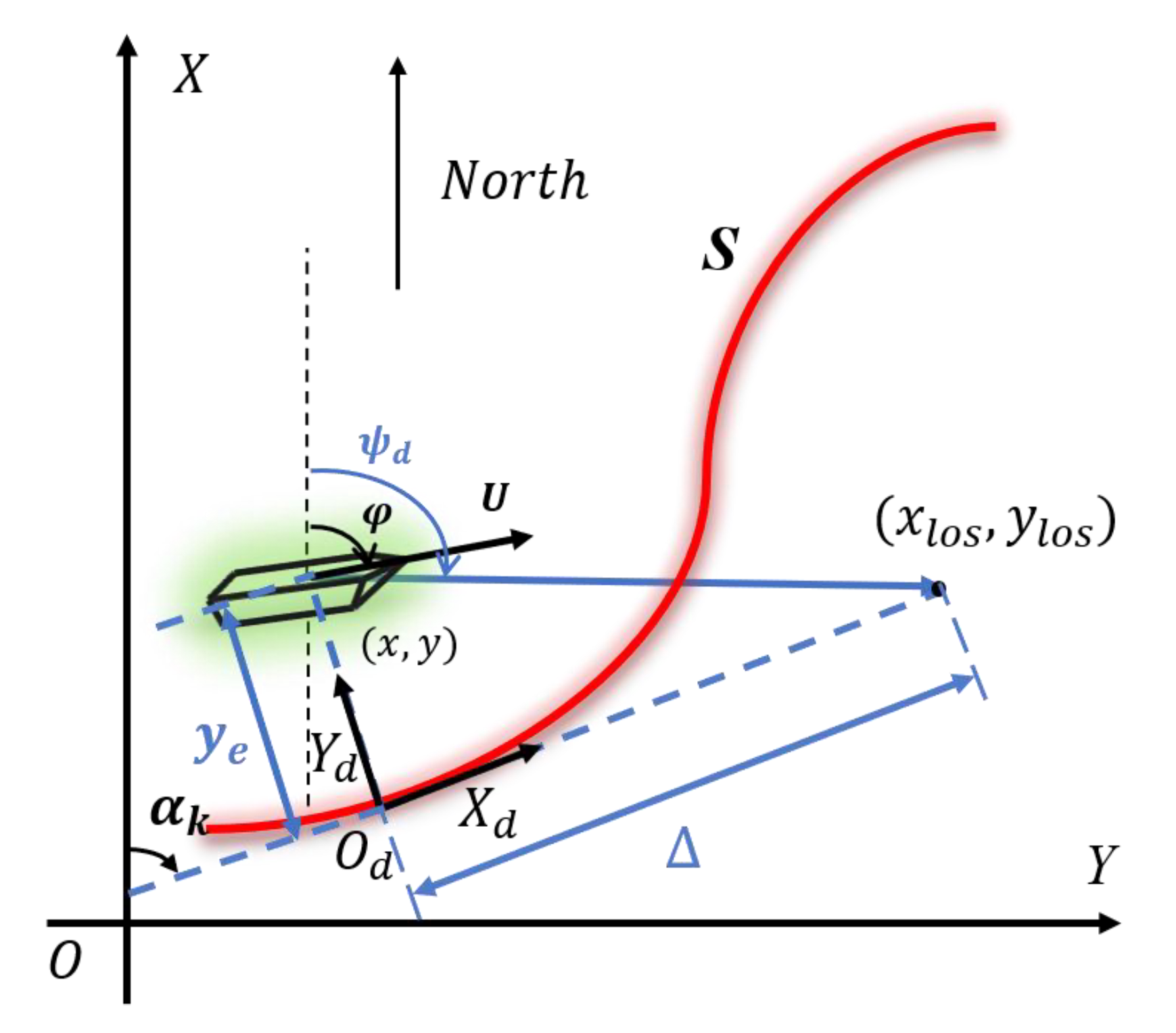
The USV path-following control problem is defined as controlling the USV to the desired path S . The line-of-sight (LOS) guidance law is a classical and effective navigation algorithm that does not depend on any dynamic control model and is insensitive to high-frequency white noise. The guidance law can efficiently calculate the desired course and pass it to the controller to achieve the control goal in real time owing to the reason that the desired course is only related to the desired route and the real-time position of the USV. LOS guidance algorithms can be divided into two types, which are based on the lookahead distance and the enveloping circle. The former type is adopted in this paper. The figure of LOS guidance law is shown in Figure 3.
The PID controller is a linear regulator that compares the desired heading angle ψ d ( t ) with the actual heading angle φ ( t ) to form the heading angle deviation e ( t ) :
e ( t ) = ψ d ( t ) φ ( t )
The desired rudder angle can be expressed as Equation (6):
δ ( k ) = K p e ( k ) + K i i = 0 k e ( i ) K d ( e ( k ) e ( k 1 ) )
Considering the integral saturation condition of the PID controller, the PD parameters are adjusted to ensure the USV quickly tends to the desired track and keeps the USV navigating within the error range. Therefore, Equation (6) can also be expressed as Equation (7),
δ = K p e + K d ( e e )
where e is the error at the last time. The neural network is performed to produce the appropriate PD parameters.

2.3. SAC Algorithm

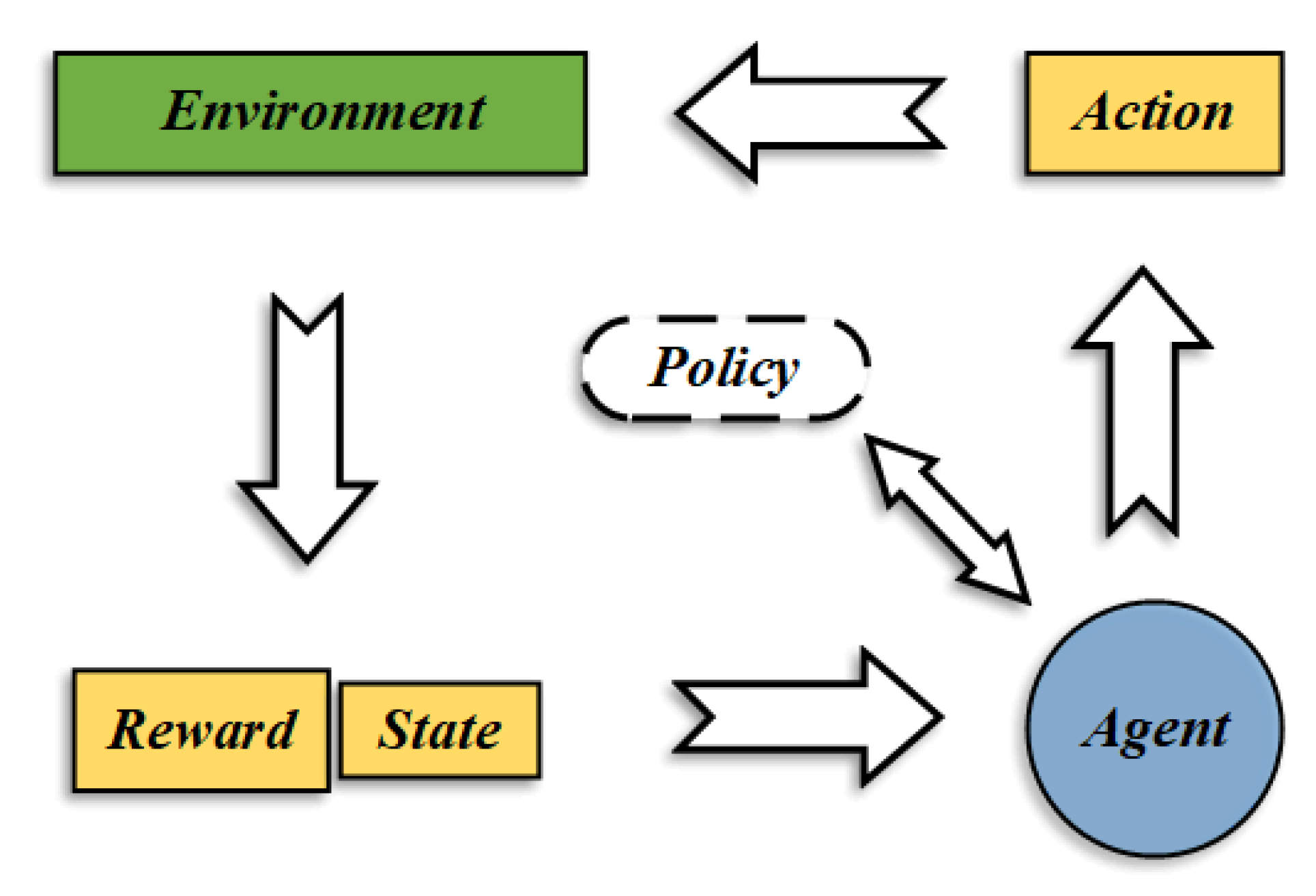
Figure 4 clearly describes the interaction process between the reinforcement learning agent and the environment, which is also called the Markov Decision Process (MDP) [25]. ( S ,   A ,   ρ ,   r ) is an important tuple in MDP, in which S is all the states in the environment, A is the set of all the actions, ρ represents the probability density of the next state, and s t + 1 S is given the current state s t S , and the action a t A . r is a bounded immediate payoff at each time when one state transfers to another. ρ π ( s t , a t ) represents the state-action distribution generated by policy π . At time t , the agent obtains the state s t from the environment and inputs it into the policy π to obtain the action a t . The action a t is executed and the reward r t of the current step is obtained, while the agent enters the next state s t + 1 . γ represents the discount factor, so the total reward at time   t can be described as Equation (8). The state value function, shown in Equation (9), can be used to evaluate the quality of the current state, while the state-action-value function, shown in Equation (10), can be used to represent whether the action made in the current state is of high quality. The transformation between these two can be described as Equations (11) and (12).
R t = k = 0 γ k r t + k
V π ( s ) = E π [ k = 0 γ k r t + k | s t = s ] = E [ R t | s t = s ]
Q π ( s , a ) = E [ R t | s t = s , a t = a ]
V π ( s ) = E [ Q π ( s , a ) | s t = s ]
Q π ( s , a ) = R t + 1 + γ s t + 1 S P s s a V π ( s t + 1 )
where P s s a = P [ s t + 1 = s | s t = s , a t = a ] , and P is a state transition probability matrix. The optimization objective in reinforcement learning is to maximize the long-term reward R. According to the MDP solution process, the optimal strategy π is the policy that maximizes the reward R , which can be described as Equation (13).
π = arg   max t = 0 T E ( s t , a t ) ρ π [ γ t r ( s t , a t ) ]
Compared with other strategies, the core idea of SAC is that entropy information which encourages the agent to explore for maximizing the entropy reward is combined with the original reward. Thus, Equation (13) can be updated as Equation (14),
π = arg   max t = 0 T E ( s t , a t ) ρ π [ γ t r ( s t , a t ) + α H ( π ( s t ) ) ]
where α is the entropy coefficient, which controls the weight between the entropy term and the revenue term and also influences the randomness of the strategy. H is entropy, which represents the randomization of the current policy, expressed as Equation (15).
H ( P ) = E x P [ log P ( x ) ]
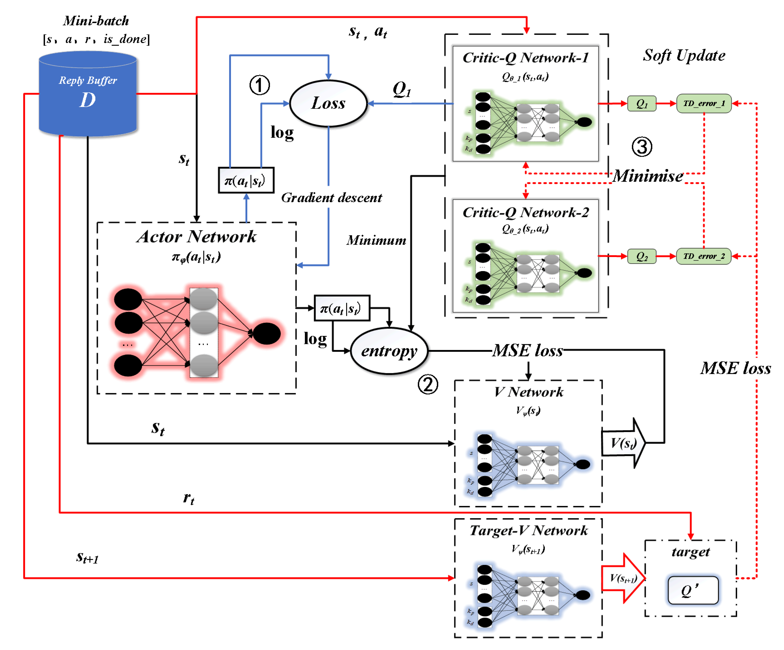
In this paper, the SAC algorithm is mainly composed of five networks, including two value networks (one V network, one target-V network), two action-value networks (Q network), and one actor network ( π network). The V network is used to calculate the value of the value function. The Q network is used to calculate the value of the action-value function. The network π outputs the policy value that guides the action of the agent. The overview of the SAC system is shown in Figure 5.

2.3.1. Training and Updating of the Actor Network

The strategy π is a Gaussian distribution with mean μ and covariance σ calculated by the neural network. The sampling of each policy π ϕ ( · | s t ) is a function calculated from the state s , policy parameter ϕ , and independent noise ξ N ( 0 , 1 ) , which can be described as Equation (16). The loss function of the actor network training is given as Equation (17).
a ˜ ϕ ( s , ξ ) = tan h ( μ ϕ ( s ) + σ ϕ ( s ) ξ )
L o s s = E ξ N [ α log   π ϕ ( a ˜ ϕ ( s , ξ ) | s ) Q ( s , a ˜ ϕ ( s , ξ ) ) ]
Compared with other RL methods, obtaining action a ˜ to calculate the L o s s instead of selecting the action from the sampled mini-batch data, the actor network is reused to predict all of the possible actions. The optimization objective of the actor network can be expressed as Equation (18). The gradient calculation formula of the actor network is expressed as Equation (19).
J π ( ϕ ) = E ξ N [ α log   π ϕ ( a ˜ ϕ ( s , ξ ) | s ) min i = 1 , 2 Q θ _ i ( s , a ˜ ϕ ( s , ξ ) )   ]
^ ϕ J π ( ϕ ) = ϕ α log ( π ϕ ( a t | s t ) ) + ( a t α log ( π ϕ ( a t | s t ) ) a t min i = 1 , 2 Q θ i ( s t , a t ) ) ϕ a ˜ ϕ ( s , ξ )

2.3.2. Training and Updating of V Networks

As shown in Figure 5, the V network is updated with the mini-batch, which is the data sampled from the experience pool. The combination of the probability π ( a t | s t ) of performing action a t in the current state s t , the probability log ( π ( a t | s t ) ) after taking the logarithm, and the minimum value of the state-action value Q 1 and Q 2 is taken as the true value of the V network. The MSE method is adopted for loss function calculation and V network training. The objective function can be expressed as Equation (20):
J V ( ψ ) = E s t D [ 1 2 ( V ψ ( s t ) E a t π ϕ [ min i = 1 , 2 Q θ i ( s t , a t ) α log π ϕ ( a t | s t ) ] ) 2 ]
where ψ is the parameter in the V network. D is the experience pool. a t π ϕ means that instead of sampling from the experience pool, the actions are sampled according to the current policy. The gradient calculation formula of the V network is expressed as Equation (21).
^ ψ J V ( ψ ) = ψ V ψ ( s t ) ( V ψ ( s t ) Q θ ( s t , a t ) + log π ϕ ( a t | s t ) )

2.3.3. Training and Updating of Critic-Q Network

As shown in Figure 5, the Q network is updated with the mini-batch, which is the data sampled from the experience pool. Q = r t + γ V ( s t + 1 ) is used to calculate the true value of the state s t , and Q 1 and Q 2 at the same action a t are used to estimate the predictive value of the state s t . The objective function can be expressed as Equation (22):
J Q ( θ ) = E ( s t , a t ) D [ 1 2 ( Q θ ( s t , a t ) Q ( s t , a t ) ) 2 ]
where θ is the parameter in the Q network. Q ( s t , a t ) is presented as Equation (23):
Q ( s t , a t ) = r ( s t , a t ) + γ E s t + 1 P [ V Ψ ¯ ( s t + 1 ) ]
where Ψ ¯ is the parameter of the target-V network in the state s t + 1 . The gradient calculation formula for the Q network is expressed as Equation (24).
^ θ J Q ( θ ) = θ Q θ ( s t , a t ) ( Q θ ( s t , a t ) r ( s t , a t ) γ V Ψ ¯ ( s t + 1 ) )
Leaving the entropy coefficient α unchanged would be unreasonable because constant change in reward would negatively affect the whole training process. Therefore, it is necessary to automatically adjust α . To improve the learning speed and improve the stability of the agent, this article designed a neural network to adaptively adjust the size of the entropy coefficient α based on the theory of reference [26]. Specifically, when the agent enters a new solution area where the agent’s exploration ability should be enhanced to find the best action, α should increase so that the agent will not be trapped in the local optimum. When the agent has almost finished the exploration in a solution area where the learning ability of the agent should be improved, to accumulate experience from the best action, α should be decreased. The optimization function maximizes the expected return under the constraint of the minimum expected entropy, which can be expressed as Equation (25):
max π 0 : T E ρ π [ t = 0 T γ t r ( s t , a t ) ] s . t .   E ( s t , a t ) ρ π [ log   ( π t ( a t | s t ) ) ] H 0 , t
where H 0 is a constant, representing the preset minimum entropy value. To solve Equation (25), the Lagrange multiplier method is performed to transform the optimization problem into the primal problem and its dual problem. Then the final optimization result can be obtained as Equation (26).
α t * = arg min α t t = 0 T E ρ t * [ α t log π t * ( a t | s t ) α t H 0 ]
where ρ t * indicates the state-action pair of the optimal policy. Then the network for α is setup and the stochastic gradient descent is performed as in Equation (26), which can be dubbed Equation (27).
^ α J ( α ) = α E a t π t [ α t log π t ( a t | s t ) α t H 0 ] α α η α J ( α )
where a t is derived from the current policy π t ( s t ) , but s t is selected from the mini-batch. The Adam algorithm is used for optimization and the learning rate l r α is set to 0.0001.

2.3.4. The Design of State, Action Space, and Reward

During path following, the USV will be disturbed by wind, waves, currents, and other environmental factors. To make the output parameters of the agent more accurate, the environmental information should be considered in the state space design as much as possible. Based on the USV model constructed in Section 2, the state space is defined as Equation (28).
s = [ u , v , r , φ , y e , α k , δ , δ ˙ , e , e ˙ ]
Similarly, the action space is defined as a = [ K p , K d ] , and K p   ranging from [ 0.5 , 0.5 ] , and K d ranges from [ 50 , 50 ] . The reward function r has two parts, one is r psi , the other is r y e ; r p s i and r y e are designed as shown in Equations (30) and (31).
r = r psi + r y e
r psi = { 0 , e 0.1 e 0.1 e , e 0.1
r y e = { 0 , y e 1 0.1 , y e 1
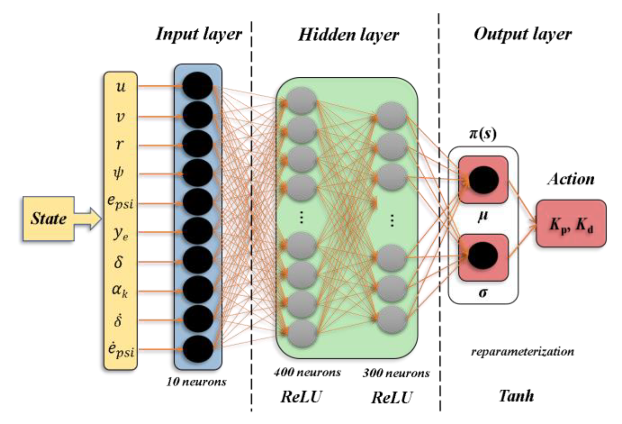
The design of the actor network and the critic network are shown in Figure 6 and Figure 7. It can be seen that they share the same structure. The dimension of the input layer in the actor network is set as 10. The hidden layer consists of two layers with 400 and 300 neuron nodes, respectively. The dimension of the output layer is set to 2. The dimension of the input layer in the critic network is set as 12. The hidden layer includes two layers with 400 and 300 neuron nodes, respectively. The dimension of the output layer is set to 1. In order to prevent gradient saturation and gradient disappearance, ReLU is used as the activation function of hidden layers in both actor and critic, and tanh is adopted as the activation function of the output layer.

3. Training and Simulation Results

3.1. Network Training

The algorithm code was written based on Pycharm (Jetbrains, Czech Republic) and TensorFlow 2.0.1 (Google Brain, USV) and was used as the framework, and the code runs on a computer with 8GB RAM. The maximum time step of each training was 2500 and the number of training runs was set to 1500. On average, it takes 154 min to complete the training for each path following. The Adam optimizer based on gradient descent was used to learn the parameters of the deep neural network during training. To test the superiority of the SAC algorithm, training and learning based on the DDPG algorithm were performed for comparison. The hyperparameters of the agents are shown in Table 3.
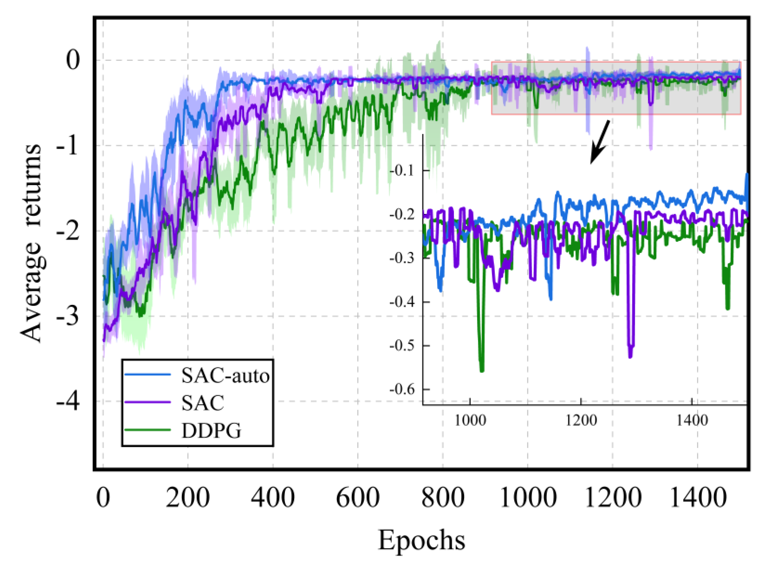
At the initial times of the network training, the strategy was almost random, and the agent could not learn much useful experience, so the effect of following the desired path was not good. Figure 8 shows the training process diagram. To better highlight the average performance and fluctuation range of the algorithm, it was designed as a mean–variance curve. The vertical coordinate was designed as the average return per 10 training sessions. The return was calculated after each training, and the parameters of each network were updated for N T times according to the reward. Note that the reward represents an immediate return on the action taken. The return is the sum of the immediate returns after the training.
It can be seen from Figure 8 that all three algorithms can converge. SAC-auto converges faster than the DDPG. The average return and mean square deviation (MSD) after training are shown in Table 4. The higher average return and smaller MSD indicate that the agent based on the SAC algorithm can better complete the path-following task and has a better stability.

3.2. Simulation Results

In this section, the effectiveness of the proposed method is verified by the linear and circular path-following simulation in the simulated wind and wave environment, where u 0 = 1.242   m / s , v 0 = 0   m / s , and r 0 = 0   m / s at the beginning. Under the same guidance law, the abovementioned control method with three trained RL parameters is compared with the adaptive PID parameter controller [28].
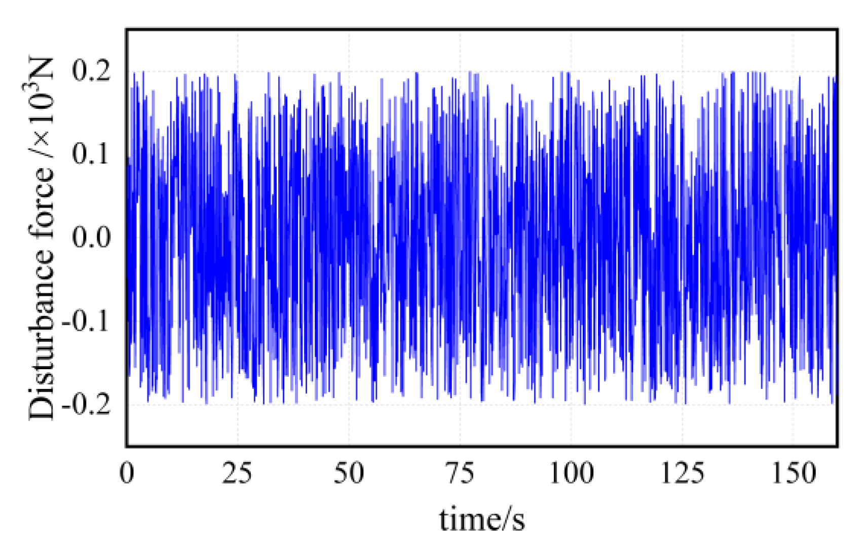
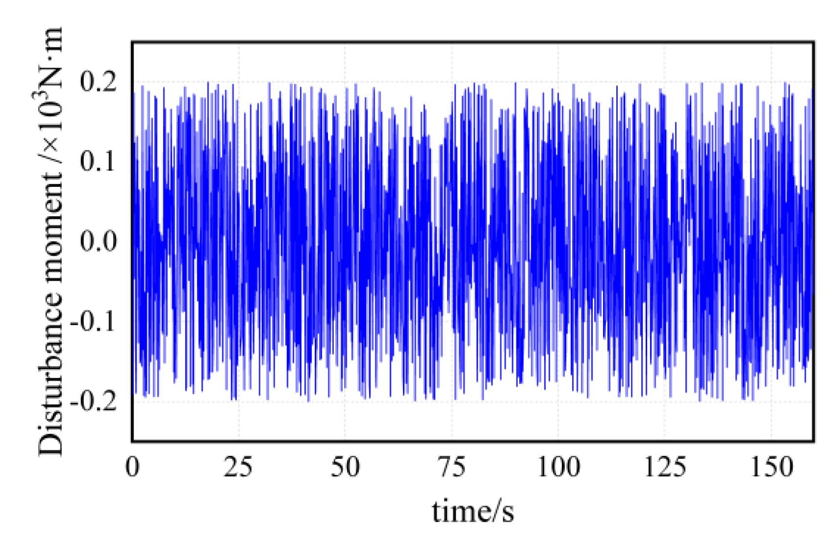
In this paper, in order to verify the anti-interference and navigation stability of the system, the interference of [ 0.2 × 10 3 ,   0.2 × 10 3 ] N was added to the transverse force, and the interference of [ 0.2 × 10 3 ,   0.2 × 10 3 ] N·m was added to the turning moment. The transverse disturbing force is shown in Figure 9. The turning disturbing moment is shown in Figure 10.

3.2.1. Linear Path Following

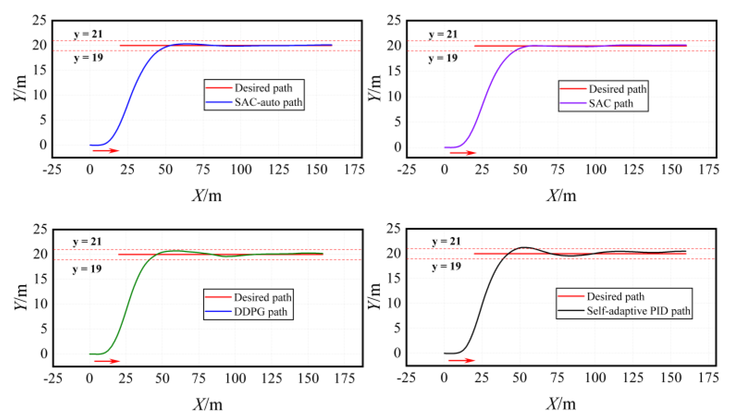
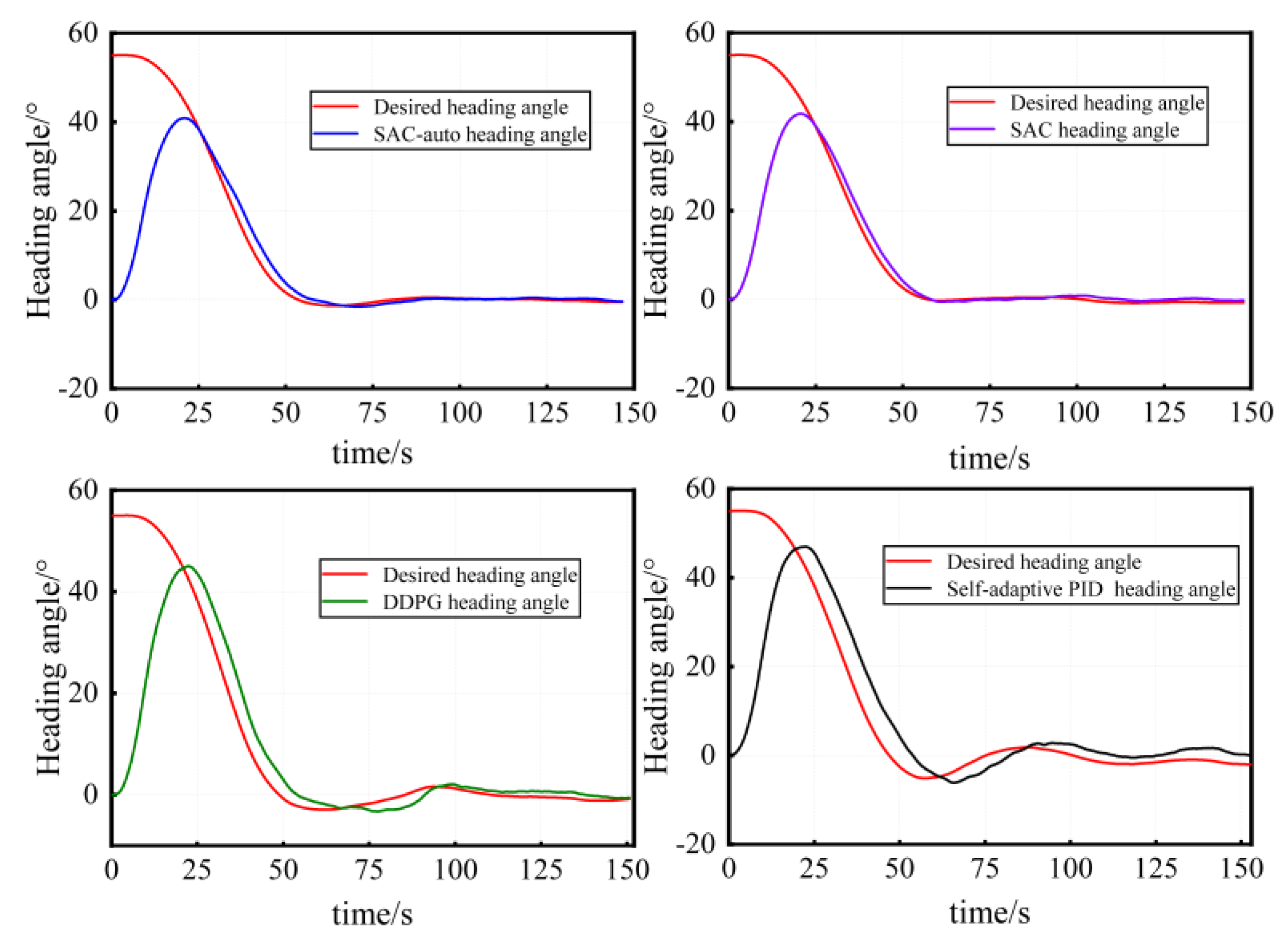
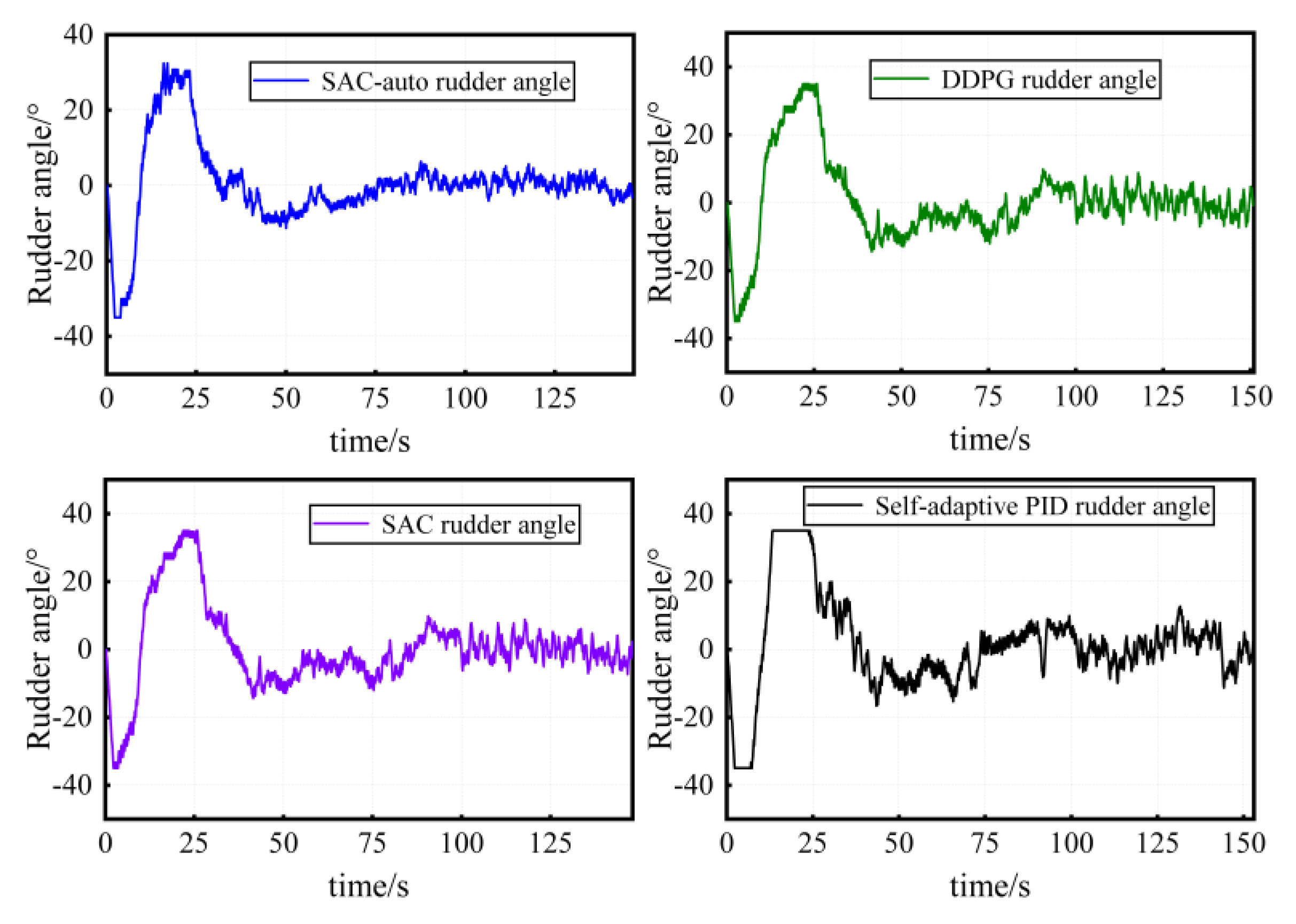
The linear reference path was designed as the line segment between the points ( 20 ,   20 ) and ( 160 ,   20 ) . The initial position of the USV is ( 0 ,   0 ) , and its initial heading is parallel to the path. Figure 11 is the path following the comparison figures between the controllers mentioned above. Figure 12 and Figure 13 are the comparisons of the heading angle and rudder angle during the path-following process. The path-tracking errors of the four controllers are shown in Table 5. The controller based on the reinforcement learning algorithm takes about 2 to 3 s to complete a path-following task, which is not much different from the calculation time in the literature [28], but the actual time still needs to prevail.
It can be seen from Figure 11 that in the presence of a disturbing force, the tracking trajectories obtained with four controllers finally approached the desired paths within the specified error range. The rudder angle is rapidly operated to overcome the disturbance of waves. Compared to the adaptive controller, the RL-based controller has less overshoot during steering and produces smoother trajectories. Compared to the DDPG algorithm controller, the SAC-auto controller has better performance in both heading control and rudder maneuvering. According to Table 5, compared to the SAC controller, the steady-state performance of the SAC-auto controller is improved, with which, when the desired direction changes, the improved parameter can provide the USV with a fast adjustment to the desired direction and a stable path-following effect on the desired path, and the average deviation of the direction angle when stable is limited to 0.5°. It can also be concluded from Figure 13 that the fluctuation of the rudder angle with SAC-auto is the smoothest, and the maximum fluctuation of the rudder angle is less than 5°, indicating that the rudder is slightly frayed and the control gear can be well-protected.
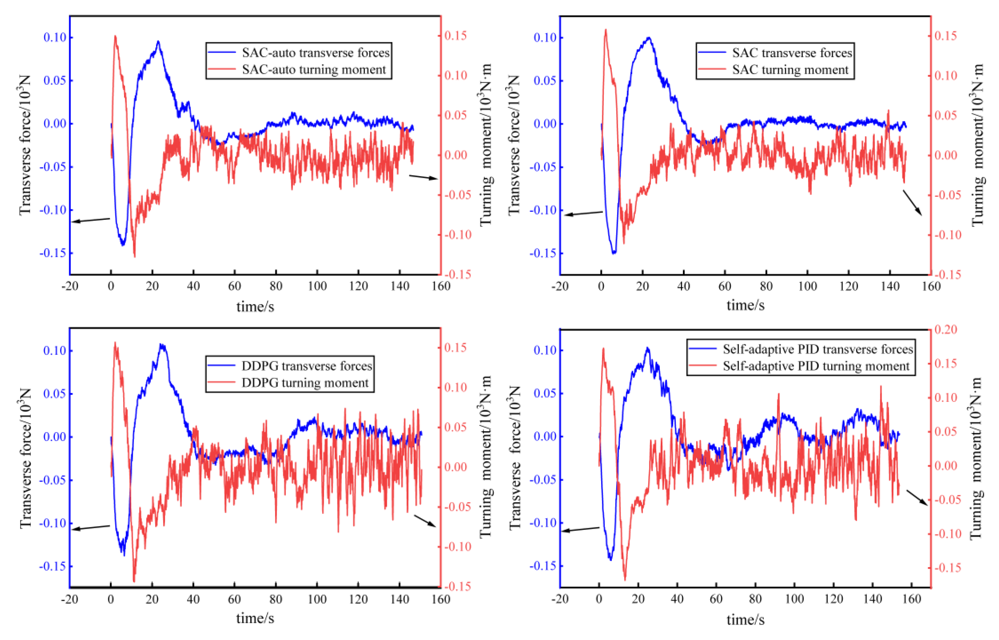
The parameter curves of K p and K d output by SAC-auto are shown in Figure 14. Figure 15 shows the transverse force and turning moment of the USV. It can be seen that under the control of the SAC-auto algorithm, the transverse force and turning moment of the USV fluctuate less; the reason is that the maneuvering fluctuation of the rudder angle is smaller.

3.2.2. Curve and Polyline Path Following

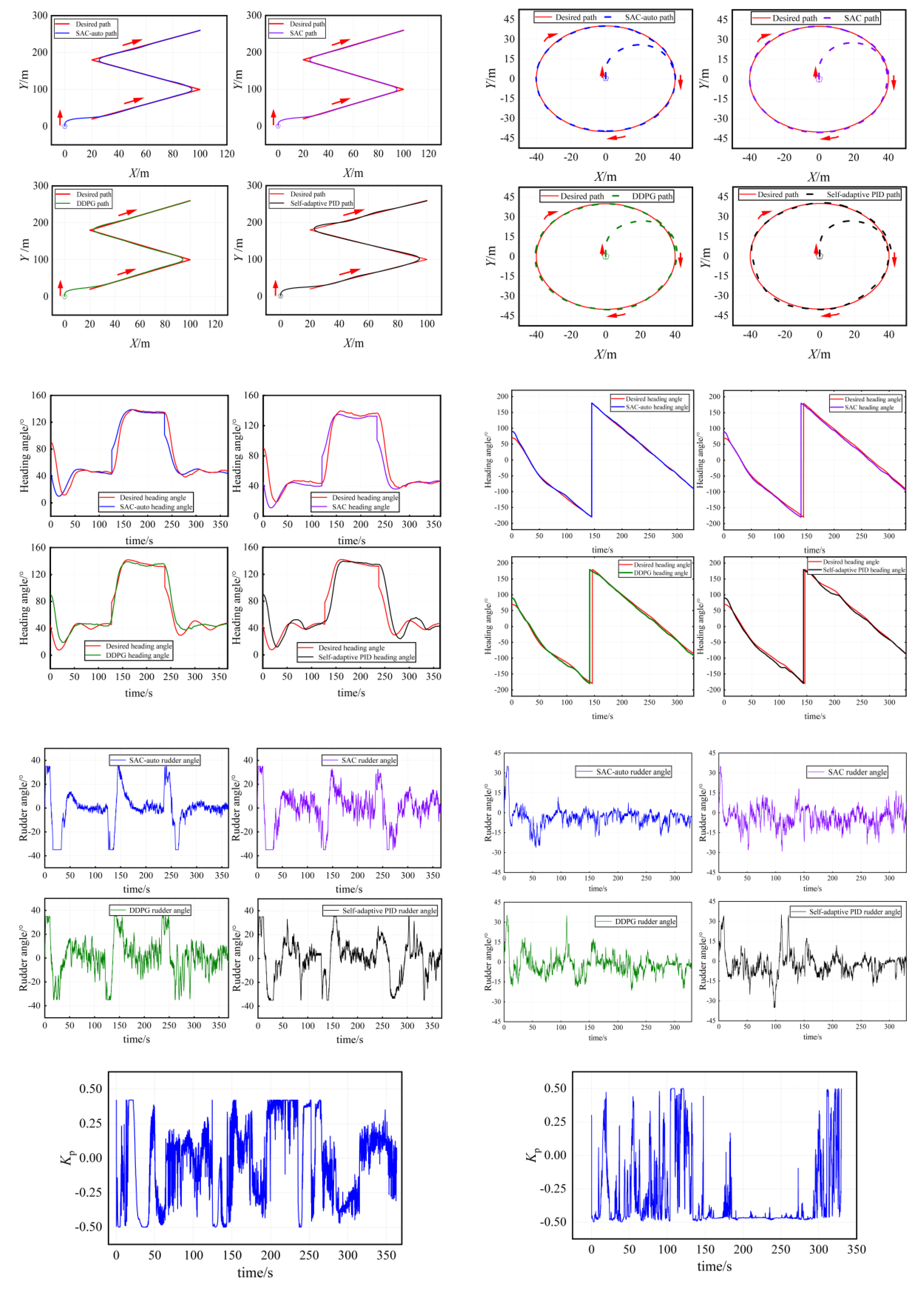
The above simulation results verify the feasibility and anti-interference ability of the SAC-auto algorithm when following a straight path. In order to verify the performance of the algorithm when following other desired paths which are more complex, and to inspect whether the SAC-auto algorithm can adaptively produce appropriate PD parameters, the path-following simulations of zigzag and turning are performed.
Scenario 1.
The desired path of the zigzag is designed as the polyline between points (20, 20), (100, 100), (180, 20), and (260, 100). The initial position of the USV is located at (0, 0), and the initial heading is parallel to the Y-axis.
Scenario 2.
The turning path is a circle with points (0, 0) as the center and 40m as the radius. The initial position of the USV is (0, 0), and the initial heading is parallel to the Y-axis.
Figure 16 shows the graphs for path following, rudder angle, heading angle, and curves of K p and K d for different algorithms in the tracking process.
It can be seen from the simulations that the SAC-auto controller has a better performance in both heading control and rudder maneuvering under the condition of path following of zigzag and turning when considering the disturbance of the wave. The fluctuation of the rudder angle with SAC-auto is the smoothest, indicating that the SAC-auto control method performs well when following a complex desired path.

4. Conclusions

The classic adaptive PID control method used for path following does not perform well under complex conditions such as following a curvilinear path or considering wave interference. Concerning this issue, this paper presents a path-following control method based on SAC for PID parameter setting. First, a 3-DOF USV dynamics model based on Abkowite was established. Second, the guidance system using the line-of-sight method and the USV heading control system in the PID controller was designed. Third, the SAC algorithm was then used, and the state space, action space, and reward function were designed for the training of the RL on the path-following scenarios; the SAC is promoted to adaptively and rapidly adjust the PID parameter during the simulation. Finally, the algorithm was proven in the simulation experiments under path following in a straight line, zigzag, and turning with disturbance of wave scenarios, which verify the feasibility and robustness of the proposed method. In further research, the experiment should be conducted.

Author Contributions

Data curation, C.X.; funding acquisition, R.G.; methodology, L.S.; software, C.X.; visualization, C.X.; oringin draft, L.H.; writing—original draft, C.X., and L.S.; writing—review and editing, J.Y. All authors have read and agreed to the published version of the manuscript.

Funding

This research received no external funding.

Institutional Review Board Statement

Not applicable.

Informed Consent Statement

Not applicable.

Data Availability Statement

Not applicable.

Conflicts of Interest

The authors declare no conflict of interest.

References

  1. Xu, F.C.; Xie, Y.L.; Liu, X.C.; Chen, X.; Han, W. Research Status and Key Technologies of Intelligent Technology for Unmanned Surface Vehicle System. In Proceedings of the International Conference on Sensing, Diagnostics, Prognostics, and Control (SDPC), Bejing, China, 5–7 August 2020; IEEE: New York, NY, USA, 2020; pp. 229–233. [Google Scholar]
  2. Song, L.F.; Shi, X.Q.; Sun, H.; Xu, K.K.; Huang, L. Collision avoidance algorithm for USV based on rolling obstacle classification and fuzzy rules. J. Mar. Sci. Eng. 2021, 9, 1321. [Google Scholar] [CrossRef]
  3. Mnih, V.; Kavukcuoglu, K.; Silver, D.; Rusu, A.A.; Veness, J.; Bellemare, M.G.; Graves, A.; Riedmiller, M.; Fidjeland, A.K.; Ostrovski, G.; et al. Human-level control through deep reinforcement learning. Nature 2015, 518, 529–533. [Google Scholar] [CrossRef] [PubMed]
  4. Silver, D.; Lever, G.; Heess, N.; Degris, T.; Wierstra, D.; Riedmiller, M. Deterministic policy gradient algorithms. In Proceedings of the International Conference on Machine Learning, PMLR 2014, Bejing, China, 22–24 June 2014; pp. 387–395. [Google Scholar]
  5. Mnih, V.; Badia, A.P.; Mirza, M.; Graves, A.; Harley, T.; Lillicrap, T.P.; Silver, D.; Kavukcuoglu, K. Asynchronous methods for deep reinforcement learning. In Proceedings of the International Conference on Machine Learning, PMLR 2016, New York, NY, USA, 20–22 June 2016; pp. 1928–1937. [Google Scholar]
  6. Haarnoja, T.; Zhou, A.; Hartikainen, K.; Tucker, G.; Ha, S.; Tan, J.; Kumar, V.; Zhu, H.; Gupta, A.; Abbeel, P.; et al. Soft actor-critic algorithms and applications. arXiv 2018, arXiv:1812.05905. [Google Scholar]
  7. Gonzalez-Garcia, A.; Castañeda, H.; Garrido, L. USV Path-Following Control Based on Deep Reinforcement Learning and Adaptive Control. In Proceedings of the Global Oceans 2020: Singapore–US Gulf Coast, Online, 5–30 October 2020; IEEE: New York, NY, USA, 2020; pp. 1–7. [Google Scholar]
  8. Zhao, Y.J.; Qi, X.; Ma, Y.; Li, Z.X.; Malekian, R.; Sotelo, M.A. Path following optimization for an underactuated USV using smoothly-convergent deep reinforcement learning. IEEE Trans. Intell. Transp. Syst. 2020, 22, 6208–6220. [Google Scholar] [CrossRef]
  9. Wang, N.; Gao, Y.; Liu, Y.J.; Li, K. Self-learning-based optimal tracking control of an unmanned surface vehicle with pose and velocity constraints. Int. J. Robust Nonlinear Control 2022, 32, 2950–2968. [Google Scholar] [CrossRef]
  10. Zheng, Y.M.; Tao, J.; Sun, Q.L.; Sun, H.; Chen, Z.Q.; Sun, M.W.; Xie, G.M. Soft Actor–Critic based active disturbance rejection path following control for unmanned surface vessel under wind and wave disturbances. Ocean. Eng. 2022, 247, 110631. [Google Scholar] [CrossRef]
  11. Feng, Z.; Pan, Z.S.; Chen, W.; Liu, Y.; Leng, J.X. USV Application Scenario Expansion Based on Motion Control, Path Following and Velocity Planning. Machines 2022, 10, 310. [Google Scholar] [CrossRef]
  12. Moreira, L.; Fossen, T.I.; Soares, C.G. Path following control system for a tanker ship model. Ocean Eng. 2007, 34, 2074–2085. [Google Scholar] [CrossRef]
  13. Lekkas, A.M.; Fossen, T.I. A time-varying lookahead distance guidance law for path following. IFAC Proc. Vol. 2012, 45, 398–403. [Google Scholar] [CrossRef] [Green Version]
  14. Liu, T.; Dong, Z.P.; Du, H.W.; Song, L.F.; Mao, Y.S. Path following control of the underactuated USV based on the improved line-of-sight guidance algorithm. Pol. Marit. Res. 2017, 24, 3–11. [Google Scholar] [CrossRef] [Green Version]
  15. Yang, Z.K.; Zhong, W.B.; Feng, Y.B.; Sun, B. Unmanned surface vehicle track control based on improved LOS and ADRC. Chin. J. Ship Res. 2021, 16, 121–127. [Google Scholar]
  16. Liu, W.; Liu, Y.; Bucnall, R. A robust localization method for unmanned surface vehicle (USV) navigation using fuzzy adaptive Kalman filtering. IEEE Access 2019, 7, 46071–46083. [Google Scholar] [CrossRef]
  17. Do, K.D. Global robust adaptive path-tracking control of underactuated ships under stochastic disturbances. Ocean Eng. 2016, 111, 267–278. [Google Scholar] [CrossRef]
  18. Dong, Z.; Wan, L.; Li, Y.; Liu, T.; Zhang, G. Trajectory tracking control of underactuated USV based on modified backstepping approach. Int. J. Nav. Archit. Ocean Eng. 2015, 7, 817–832. [Google Scholar] [CrossRef] [Green Version]
  19. Zhou, W.; Wang, Y.; Ahn, C.K.; Cheng, J.; Chen, C. Adaptive fuzzy backstepping-based formation control of unmanned surface vehicles with unknown model nonlinearity and actuator saturation. IEEE Trans. Veh. Technol. 2020, 69, 14749–14764. [Google Scholar] [CrossRef]
  20. Ashrafiuon, H.; Muske, K.R.; McNinch, L.C.; Soltan, R.A. Sliding-mode tracking control of surface vessels. IEEE Trans. Ind. Electron. 2008, 55, 4004–4012. [Google Scholar] [CrossRef]
  21. Sun, Z.J.; Zhang, G.Q.; Qiao, L.; Zhang, W.D. Robust adaptive trajectory tracking control of underactuated surface vessel in fields of marine practice. J. Mar. Sci. Technol. 2018, 23, 950–957. [Google Scholar] [CrossRef]
  22. Guo, B.Z.; Zhao, Z.L. Active Disturbance Rejection Control for Nonlinear Systems: An Introduction; John Wiley & Sons: Hoboken, NJ, USA, 2016. [Google Scholar]
  23. Miao, R.; Dong, Z.; Wan, L.; Zeng, J. Heading control system design for a micro-USV based on an adaptive expert S-PID algorithm. Pol. Marit. Res. 2018, 25, 6–13. [Google Scholar] [CrossRef] [Green Version]
  24. Wang, J.H.; Zhao, M.K. Simulation of path following optimization control of unmanned surface vehicle. Comput. Simul. 2016, 33, 362–367. [Google Scholar]
  25. Fan, Y.S.; Guo, C.; Zhao, Y.S.; Wang, G.F.; Shi, W.W. Design and verification of straight-line path following controller for USV with time-varying drift angle. Chin. J. Sci. Instrum. 2016, 37, 2514–2520. [Google Scholar]
  26. Xu, P.F.; Cheng, C.; Cheng, H.X.; Shen, Y.L.; Ding, Y.X. Identification-based 3 DOF model of unmanned surface vehicle using support vector machines enhanced by cuckoo search algorithm. Ocean Eng. 2020, 197, 106898. [Google Scholar] [CrossRef]
  27. Budak, G.; Beji, S. Controlled course-keeping simulations of a ship under external disturbances. Ocean Eng. 2020, 218, 108126. [Google Scholar] [CrossRef]
  28. Wang, L.; Xiang, J.L.; Wang, H.D. Local Path Planning Algorithm for Unmanned Surface Vehicle Based on Improved Bi-RRT. Shipbuild. China 2020, 61, 21–30. [Google Scholar]
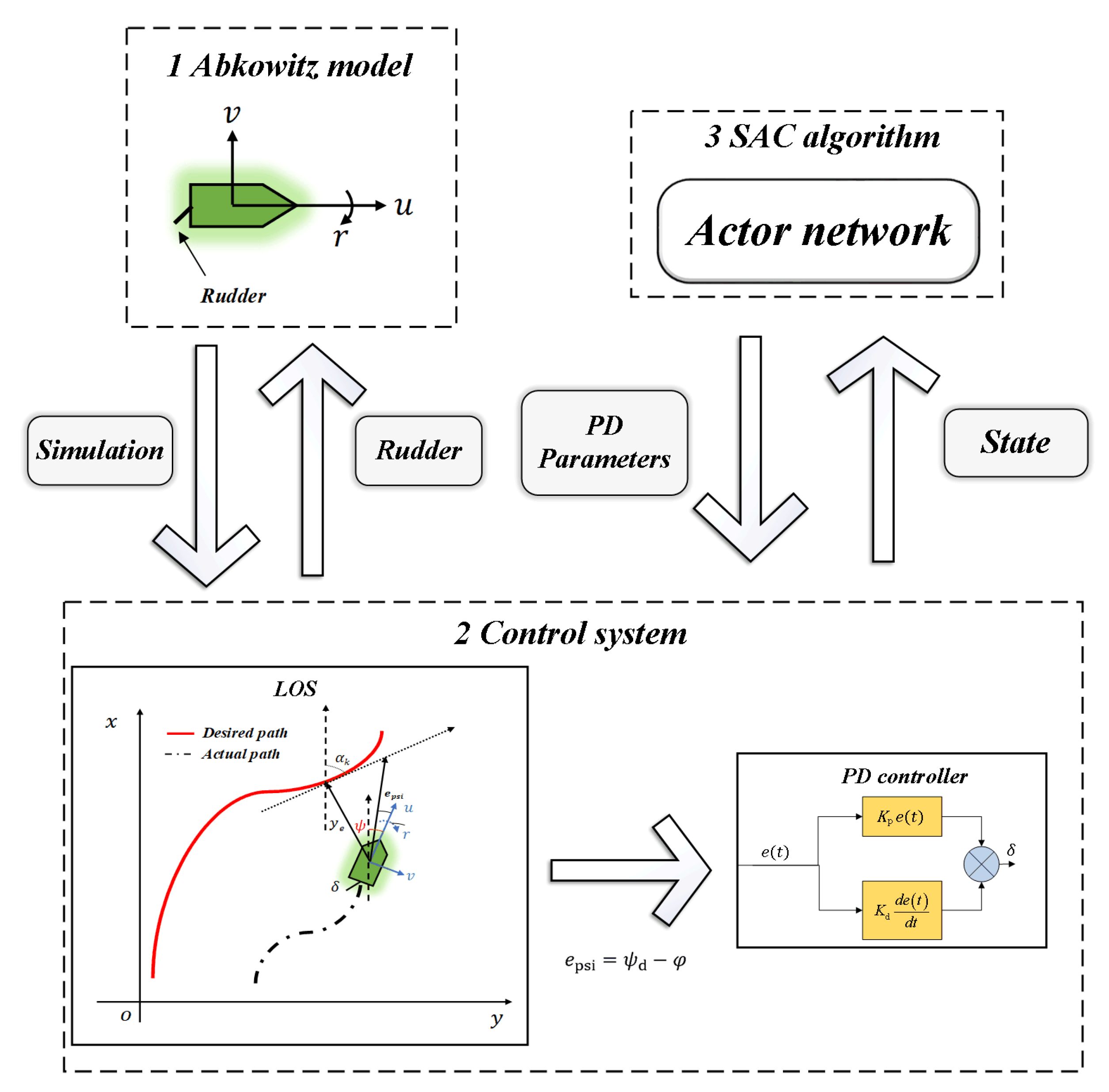
Figure 1. The overall flow diagram for the proposed method.
Jmse 10 01847 g001
Figure 2. USV manipulation motion coordinate system. u ,   v , and r are the velocities on the three degrees of freedom (forward, lateral, and head) of the ship motion, respectively. ψ is the heading angle.
Jmse 10 01847 g002
Figure 3. LOS guidance law. o x y is the global coordinate system. o d x d y d is the carrier coordinate system. ψ d is the desired heading angle. φ is the angle between the bow of the USV and the vertical axis of the global coordinate system. y e is the lateral error about path tracking. α k is the tangential angle at the o d point on the desired path. U is the actual velocity of the USV. Δ is the lookahead distance, usually set as an integer multiple of the ship’s length. In this paper, we take the multiple as 2.
Jmse 10 01847 g003
Figure 4. Schematic diagram for reinforcement learning.
Jmse 10 01847 g004
Figure 5. SAC architecture.
Jmse 10 01847 g005
Figure 6. Actor network architecture.
Jmse 10 01847 g006
Figure 7. Critic network architecture.
Jmse 10 01847 g007
Figure 8. Training process.
Jmse 10 01847 g008
Figure 9. Transverse disturbing force.
Jmse 10 01847 g009
Figure 10. Turning disturbing moment.
Jmse 10 01847 g010
Figure 11. Path following.
Jmse 10 01847 g011
Figure 12. Heading angle.
Jmse 10 01847 g012
Figure 13. Rudder Angle.
Jmse 10 01847 g013
Figure 14. Kp, Kd curves.
Jmse 10 01847 g014
Figure 15. Transverse forces and turning moments.
Jmse 10 01847 g015
Figure 16. Zigzag and circle path following, heading angle, rudder angle, and Kp, Kd curves.
Jmse 10 01847 g016aJmse 10 01847 g016b
Table 1. Main parameters of the USV.
ParametersValues
USV Weight m 3.273 t
Length L 7.0 m
Width b 1.27 m
Draught Depth T 0.455 m
Motor Rated Speed t r 16.687°/s
Designed speed u 0 1.242 m/s
Moment of inertia I z 10.0178 Kg·m2
Center of gravity x G 0.2485 m
Table 2. Hydrodynamic Coefficients.
ParametersValuesParametersValues
X u ˙ −0.00135 X v δ 0.001609
Y v ˙ −0.014508 X r δ −0.001034
Y r ˙ −0.001209 Y v −0.019
N v ˙ −0.000588 Y v v v −0.129
N r ˙ −0.000564 Y r 0.005719
X u −0.0022 Y r r r −0.000048
X u u 0.0015 Y v r r −0.02429
X u u u 0.0 Y v v r 0.0211
X v v 0.00159 Y δ 0.00408
X r r 0.000338 Y δ δ δ −0.003059
X v r 0.01391 Y u δ −0.00456
X δ δ −0.00272 Y v δ δ 0.00326
N v −0.007886 Y v v δ 0.003018
N v v v 0.000175 Y r δ δ −0.002597
N r −0.003701 Y r r δ 0.000895
N r r r −0.000707 N δ −0.001834
N v r r 0.00372 N δ δ δ 0.001426
N u δ 0.00232 N v δ δ −0.001504
N v v δ −0.001406 N r δ δ 0.001191
N r r δ −0.000398
Table 3. Hyperparameters of the algorithms.
AgentDDPGSACSAC-Auto
Discount factor γ 0.990.990.99
Hidden layer 1400400400
Hidden layer 2300300300
Activation functionReLUReLUReLU
Batch size100100100
Experience pool capacity106106106
τ 0.00010.00010.0001
lr a 0.0010.0010.001
lr c 0.0010.0010.001
α none0.2auto
Table 4. Comparison of results after training.
AgentDDPGSACSAC-Auto
Average return−0.263−0.248−0.190
MSD0.1160.0780.05
Table 5. Data comparison table of four algorithms.
ControllerTransverse Error Mean/(m)Heading Deviation Mean/(°)Average Operation Time per Step/(ms)
SAC-auto0.1280.2211.63
SAC0.1360.3761.65
DDPG0.2920.8881.61
Self-adaptive PID0.4492.0851.89
Publisher’s Note: MDPI stays neutral with regard to jurisdictional claims in published maps and institutional affiliations.