A Decision-Support Model for the Generation of Marine Green Tide Disaster Emergency Disposal Plans

Abstract

Green tide is a harmful marine ecological phenomenon caused by the explosive proliferation or high aggregation of some macroalgae, and can cause significant impacts on ecological environments and economies. An effective emergency disposal plan can significantly improve disposal capacity and reduce total costs. At present, the formulation of emergency disposal plans for green tide disasters usually depends on subjective experience. The primary purpose of this paper is to develop a decision-support model based on intelligent algorithms to optimize the type and number of resources when making emergency disposal plans so as to improve the reliability and efficiency of decision making. In order to simulate the decision-making environment more realistically, the drift motion of green tide is considered in this model. Two intelligent algorithms, the Genetic Algorithm (GA) and the improved Non-Dominated Sorting Genetic Algorithm-II (IMNSGA-II), are used to solve the model and find appropriate emergency disposal plans. Finally, a case study on the green tide disaster that occurred in Qingdao (Yellow Sea, China) is conducted to demonstrate the effectiveness and optimization of the proposed model. Through the model proposed in this paper, the overall response time and cost can be reduced in green tide disaster emergency operations.

1. Introduction

As a new type of marine disaster, massive green tides have frequently recurred in many coastal regions worldwide [1]. These floating macroalgae will grow rapidly if they are not salvaged and removed in time, which negatively impacts the ecological environment and economy of coastal areas [2,3]. For example, over USD 2.91 million has been spent every year on the cleanup of Sargassum from Texas beaches [4]. However, improper emergency disposal plans can not only reduce the efficiency of algae salvaged but also result in wasted manpower and budget. Therefore, an effective emergency disposal plan is needed in order to control the spread of green tide disasters and reduce the impact on the environment.

A typical example is the green tide disaster that occurred in the Yellow Sea of China in 2008, with a total cleanup cost of over CNY 200 million [5]. After the green tide disaster occurred, the Chinese government immediately activated the local emergency response system, and quickly took measures to control and salvage the algae. In response to the emergency, over 20,000 personnel and 1200 vessels were mobilized, and more than 1 million tons of algae were salvaged ashore [6,7]. Since 2008, green tide disasters of different scales have occurred in the Yellow Sea from May to August every year [8]. The frequent green tide disasters have attracted the attention of the government and the research community. Consequently, tremendous amount of research effort has been made in the field of green tide disaster monitoring and early warning [9,10,11,12]. In comparison, there are few studies which are devoted to how to quickly formulate an executable emergency disposal plan in the process of emergency response to green tide disasters.

The purpose of formulating the emergency disposal plan is to establish a unified, rapid, coordinated, and efficient disaster emergency disposal mechanism. The emergency strategy should be dynamically adjusted according to the needs of emergency disposal and the preferences of decision makers. As a hot topic in the field of emergency management, emergency response to maritime accidents is attracting the attention and research of many domestic and foreign scholars. Huang et al. formulated a post-disaster emergency rescue resource-allocation model with a multi-objective optimization approach [13]. Xiong et al. proposed a decision-support method for marine rescue resource scheduling [14]. Garrett et al. developed a mixed-integer linear programming model based on the time period planning horizon to solve the problem of scheduling emergency resources for oil spills [15]. In order to mitigate the ship collision risk, some studies have proposed a quantitative real-time multi-ship collision-risk analysis and collision-avoidance decision-making model which can provide good collision-risk warning and decision support [16]. At present, the disposal of green tide still adopts manual and mechanical methods. By commanding and scheduling vessels to clean up algae floating on the sea surface, the green tide blooming scale can be reduced. To mitigate the damage to the ecological environment and the threat to coastal areas caused by green tide disasters, the relevant departments need to coordinate emergency disposal efforts to make the best use of available manpower and budget. Due to the unique characteristics of green tide disasters and the limited available decision-support systems, the evaluation and selection of salvage vessels usually depend on subjective experience in emergency disposal efforts. In addition, decision makers will spend a lot of time on making decisions without any decision support. Hence, it is more urgent and crucial to improve the efficiency and reliability of decision making.

During an emergency response to a green tide disaster, the space of resource allocation is complicated and large, and the drifting characteristics of the green tide affect decision making. Therefore, determining in a short time how many and which types of resources are required is a nonlinear decision-making problem. Intelligent algorithms are an important tool for solving such problems and have a wide range of applications in emergency decision making [17,18,19,20]. Yi and Kumar presented an ant colony optimization element heuristic algorithm for solving emergency logistics issues [21]. Ye et al. developed a dynamic spill-response decision-making approach with simulation-based multi-agent and particle swarm optimization [22]. Yannibelli and Amandi introduced a hybrid search optimization algorithm based on an annealing algorithm and a multi-objective evolutionary algorithm to solve the scheduling problem [23]. There are many kinds of intelligent algorithms, but many algorithms are prone to fall into local optima or have some shortcomings in stability. The Genetic Algorithm is a general algorithm for search and optimization. Compared with other optimization methods, the advantages of the Genetic Algorithm are that it is easy to implement and has higher robustness [24]. However, Genetic Algorithm efficiency is limited by premature convergence with local minima [25]. To overcome these limitations, the Non-Dominated Sorting Genetic Algorithm-II (NSGA-II) is improved in this study to solve the emergency decision-making problem in green tide disasters. In this paper, considering the disposal capacity and total cost, the formulation of the emergency disposal plan is modeled as a multi-objective optimization problem. The improved Non-Dominated Sorting Genetic Algorithm-II (IMNSGA-II) is used to find the Pareto solutions set for optimizing the number and types of available resources. Additionally, the Technique for Order of Preference by Similarity to Ideal Solution (TOPSIS) can help decision makers select the compromise solution from the Pareto solutions set. The main contributions of this paper can be summarized as follows: (1) A decision-support model based on intelligent algorithms is developed to optimize the green tide disaster emergency disposal plan, which can improve the reliability and efficiency of decision making compared with the traditional empirical judgment; (2) The drift motion of green tide is taken into consideration in the decision-making process for the emergency response; (3) Two intelligent algorithms were introduced to find optimal emergency disposal plans about the required types and number of resources considering the disposal capacity and the total cost; (4) In order to improve the quality of decision making, an adaptive crossover mutation operator is introduced into NSGA-II to improve the performance of the algorithm.

The rest of the paper is organized as follows. Section 2 describes the problem definition and model-related concepts. In Section 3, the decision-support model in response to the green tide disaster is developed. In Section 3.5, the single-objective optimization model is outlined first, which only considers disposal capacity. Based on the single-objective model, Section 3.6 extends it to a multi-objective model, considering both disposal capacity and total cost. The algorithm for solving the model is presented in Section 4. In Section 5, the proposed model is applied in a case study to verify the effectiveness and optimization of the model. Finally, the conclusions are presented in Section 6.

2. Background to the Problem

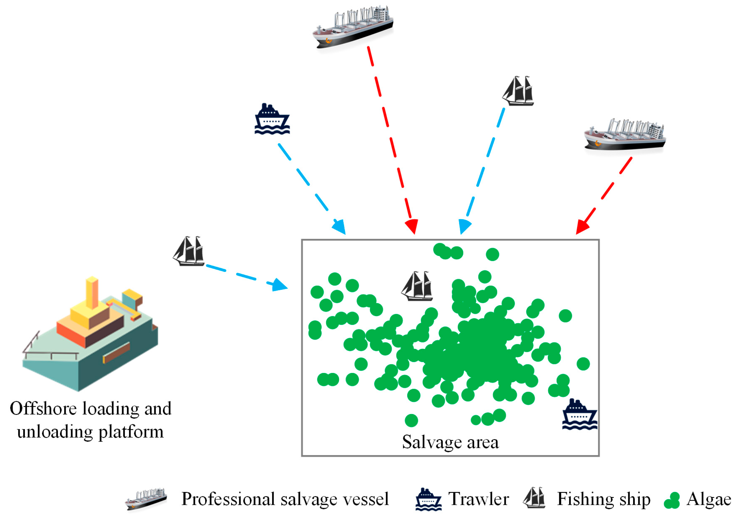
2.1. Problem Description

One of the main phases of green tide disaster emergency response is the disposal phase. In the disposal stage, how to select available resources to carry out the salvage task and achieve the most reasonable emergency disposal plan is an important issue. Before emergency disposal, the salvage area is determined by decision makers. Considering that the distribution of green tide is relatively scattered, the salvage area is generally a regular rectangle or circle. As shown in Figure 1, it was assumed that there are available fishing ships and professional salvage vessels around the salvage area. Among them, the location, speed, maximum cargo capacity, salvage efficiency, etc., of available resources are different. In order to save round-trip time, offshore loading and unloading platforms are usually located in nearby sea areas. Here, we describe the practical problem as how to find optimal emergency disposal plans about the required types and number of resources, so as to improve the disposal capacity for large-scale marine green tide disasters and reduce the total cost.

Decision-makers should pay attention to the drifting characteristics of the green tide when making emergency disposal plans. The positions of the green tide constantly change due to drift motion, which will lead to the distance between the salvage vessel and the salvage area being a time-varying parameter. Therefore, the drift characteristics of green tide will affect the decision-making of emergency disposal plans.

2.2. Green Tide Drift Prediction

The basic process of green tide drift prediction is to obtain the distribution information of green tide through advanced remote sensing monitoring technology and a geographic information system (GIS), and input the distribution information in the form of points into the numerical simulation program. Then, the drift trajectory of the green tide is predicted by calculating the drift positions of these points. The drift motion of green tide is mostly affected by the sea surface wind and surface flow [26]. Without considering the growth process of the green tide, the Lagrange particle tracking algorithm is used to simulate the drift trajectory of the green tide [27,28]. The drift velocity of the green tide center can be formulated as follows:

$$\overrightarrow{V}={\overrightarrow{v}}_t+a{\overrightarrow{v}}_w$$

(1)

where, $\overrightarrow{V}$ is the drift velocity of the green tide center, ${\overrightarrow{v}}_t$ is the surface flow velocity, ${\overrightarrow{v}}_w$ is the sea surface wind velocity, $a$ is the wind empirical coefficient.

The marine dynamic environmental data used in this paper include wind and current data. The wind field data were acquired from the European Center for Medium-Range Weather Forecasts (ECMWF), and the flow field data are from the National Marine Environmental Forecasting Center. The wind field and current field data collection process was as follows. According to the selected geographical area, data requests were made to obtain NC (NetCDF, Network Common Data Form) files. Then, the NC file was preprocessed. Finally, the data in GeoJSON format containing marine environment information were generated for analysis. In this paper, wind and flow data are used to calculate the drift velocity of the green tide center.

3. Methodology: A Decision-Support Model for Green Tide Disasters

In order to obtain the optimal emergency disposal plan, we need not only to improve the emergency disposal capacity but also to reduce the cost. Aiming at this goal, we construct the single-objective and multi-objective models. The single-objective model concerns the disposal capacity only. The multi-objective model helps to ensure both the disposal capacity maximization and total cost minimization. The multi-objective model can provide more options depending on the decision-making preference. In addition, our model can cope with the complexity of the decision-making process caused by the time-varying conditions of green tide drift.

3.1. Assumptions

(1)

Prior to making decisions regarding emergency disposal, the distribution and biomass of green tides have been determined, and green tides will not grow during emergency disposal efforts.

(2)

The maritime environment remains stable during the emergency disposal efforts, so the drift speed of green tide remains constant.

(3)

Salvage vessels may perform several round trips between the offshore loading and unloading platform and the salvage area to unload the salvaged algae. The offshore loading and unloading platform has sufficient cargo capacity.

(4)

The model does not account for the unloading time of the algae. Since the tonnage of emergency disposal vessels is generally small, there is no obvious difference in the overall unloading time.

3.2. Decision Variables

The result of the decision is the type and number of specific resources. To express the emergency disposal plan more intuitively, we express the emergency disposal plan $X$ as a vector. The value of the $i^{th}$$(i\le I)$ dimensional space of vector $X$ is $x_i$, which is the decision variable. The mathematical expression of vector $X$ is:

$$X=(x_1,x_2,x_3,.\dots \dots x_I)$$

(2)

where $I$ indicates the total types of available resources, and $x_i$ is the number of resource $i$ participating in the green tide disaster emergency operations. If the value of $x_i$ is 0, then the resource $i$ is not selected to participate in emergency disposal efforts.

3.3. Model Parameters

Table 1. Parameters of the model.

Parameter	Description
$M$	$\mathrm{Biomass}\mathrm{of}\mathrm{green}\mathrm{tide}\mathrm{in}\mathrm{salvaged}\mathrm{area}(\mathrm{ton})$
$Q$	Maximum number of salvage vessels that can be accommodated in the salvage area
$V$	$\mathrm{The}\mathrm{drift}\mathrm{velocity}\mathrm{of}\mathrm{green}\mathrm{tide}(\mathrm{nmi}/\mathrm{h})$
$B$	$\mathrm{Current}\mathrm{sea}\mathrm{state}\mathrm{level}(B\in \{0,1,\cdots ,9\})$
$ct$	$\mathrm{Transportation}\cos \mathrm{t}\mathrm{of}\mathrm{the}\mathrm{salvage}\mathrm{vessel}\mathrm{per}\mathrm{nautical}\mathrm{mile}(\mathrm{CNY})$
$b_i$	$\mathrm{The}\mathrm{safe}\mathrm{sea}\mathrm{state}\mathrm{levels}\mathrm{of}\mathrm{resource}i$
$G_i$	$\mathrm{The}\mathrm{geographic}\mathrm{coordinates}\mathrm{of}\mathrm{resource}i$
$n_i$	$\mathrm{The}\mathrm{maximum}\mathrm{available}\mathrm{number}\mathrm{of}\mathrm{resources}i$
$v_i$	$\mathrm{The}\mathrm{speed}\mathrm{of}\mathrm{resource}i$$(\mathrm{nmi}/\mathrm{h})$
$Ma{x}_i$	$\mathrm{The}\mathrm{maximum}\mathrm{cargo}\mathrm{capacity}\mathrm{of}\mathrm{resource}i$$(\mathrm{ton})$
$sa{l}_i$	$\mathrm{The}\mathrm{salvage}\mathrm{efficiency}\mathrm{of}\mathrm{resource}i$$(\mathrm{ton}/\mathrm{h})$
$F{C}_i$	$\mathrm{The}\mathrm{fixed}\mathrm{operating}\cos \mathrm{t}\mathrm{of}\mathrm{resource}i$$(\mathrm{CNY})$
$t_i$	$\mathrm{Duration}\mathrm{of}\mathrm{resource}i$ from its current position to the salvage area
$T_i$	$\mathrm{Moment}\mathrm{when}\mathrm{resource}i$ is to leave its current position for the salvage area
$di{s}_i(t)$	$\mathrm{Distance}\mathrm{between}\mathrm{resource}i$$\mathrm{and}\mathrm{the}\mathrm{salvage}\mathrm{area}\mathrm{at}\mathrm{time}t$

lists the parameters of the model and their detailed descriptions. Except for some certain capabilities, most of them can be obtained directly. Experience shows that we can obtain this information through historical data. We assumed that they are known in our model.

3.4. Constraints

(1)

To ensure that salvage vessels are working under a safe environment, the maximum allowable sea state of resource $i$ should be greater than the current sea state level:

$$b_i\ge B,b_i\in \{0,1,\cdots ,9\},i=1,2\cdots ,I$$

(3)

(2)

During the salvage process, the number of vessels that can be accommodated in the salvage area is limited. Overcrowding between vessels will limit the range of activities of the vessels, thus affecting the efficiency of algae salvaged. At the same time, overcrowding between vessels can also lead to vessel collisions, thus causing accidents. Therefore, the total number of resources selected must be less than or equal to the maximum number of vessels that can be accommodated in the salvage area.

$$Q\ge {\displaystyle \sum _{i=1}^I{x}_i},i=1,2\cdots ,I$$

(4)

(3)

Due to the drift of the green tide, the distance between the vessel and the salvage area is constantly changing. Here, we use a mathematical derivation to determine the travel time when the vessel meets the salvage area. The positions of the nodes at sea are shown in Figure 2, where $a_i$ is the position of resource $i$, $a_j$ is the position of salvage area, and $a_j^{*}$ is where resource $i$ meets salvage area. Based on the cosine theorem, the following equation is formulated:

$$\begin{array}{l}{(v_i\cdot t_i)}^2=di{s}_i^2(T_i)+{(V\cdot t_i)}^2-2\cdot di{s}_i(T_i)\cdot V\cdot t_i\cdot \cos \lambda \\ \Rightarrow t_i=\frac{-v_i\cdot di{s}_i(T_i)\cdot \cos \lambda \pm di{s}_i(T_i)\cdot \sqrt{v_i^2-V^2\cdot {\sin }^2\lambda }}{v_i^2-V^2}\end{array}$$

(5)

According to Equation (5), the following speed constraint shall be met when resource $i$ is able to reach the salvage area:

$$v_i^2-V^2\cdot {\sin }^2\lambda \ge 0\Rightarrow v_i\ge V\cdot \sin \lambda$$

(6)

(4)

To allocate time reasonably, the moment when resource $i$ first arrives at salvage area should be less than the maximum working time, which is defined as 12 h in this model:

$$12>\frac{-v_i\cdot di{s}_i(0)\cdot \cos \lambda \pm di{s}_i(0)\cdot \sqrt{v_i^2-V^2\cdot {\sin }^2\lambda }}{v_i^2-V^2}$$

(7)

3.5. The Single-Objective Model

The disposal capacity is considered as the objective function during the single-objective optimization. In this paper, the disposal capacity is defined as the total amount of algae salvaged within the first 12 h period. The time of resource $i$ participating in green tide emergency disposal efforts within 12 h is shown in Figure 3. For an emergency disposal plan $X=(x_1,x_2,x_3,.\dots \dots x_I)$, the calculation formula of the objective function $f_1$ is as follows.

$$f_1={\displaystyle \sum _{i=1}^I{x}_i\cdot T_{si}\cdot sa{l}_i}$$

(8)

$$T_{si}={\{\begin{array}{l}n\cdot {\widehat{T}}_i,{\overline{T}}_i\ge {\widehat{T}}_i\\ (n-1)\cdot {\widehat{T}}_i+{\widehat{T}}_i,{\overline{T}}_i<\widehat{T}\end{array}}_i$$

(9)

$${\widehat{T}}_i=\frac{Ma{x}_i}{sa{l}_i}$$

(10)

$${\overline{T}}_i=12-T_i^n-t_i^n$$

(11)

where $T_{si}$ is the total salvage time of the resource $i$ within 12 h. ${\widehat{T}}_i$ is the duration from the beginning of salvage to the full load of the resource $i$. ${\overline{T}}_i$ is the remaining time after the resource $i$ arrives at the salvage area for the nth time.

3.6. The Multi-Objective Model

In the emergency disposal of green tide disasters, it is also very important to effectively balance the disposal capacity and total cost. The total cost generated in the process of emergency disposal to green tide disasters includes the fixed operating cost of a vessel ($C_1$) and the vessel travel cost ($C_2$). For a vessel scheduling scheme $X=(x_1,x_2,x_3,.\dots \dots x_I)$, the calculation formula of the objective function $f_2$ is as follows.

$$f_2=C_1+C_2$$

(12)

$$C_1={\displaystyle \sum _{i=1}^I{x}_i\times F{C}_i}$$

(13)

$$C_2={\displaystyle \sum _{i=1}^I{x}_i\cdot v_i\cdot ct\cdot 12}$$

(14)

To turn the decision objective into the multi-objective minimization problem, the value of $f_1$ is set to the opposite number here. Hence, the mathematical expression of the multi-objective optimization problem is described as: $\min [-f_1(X),f_2(X)]$.

4. Algorithm Design and Model Solving

When making an emergency disposal plan, the problem of optimizing number and types of resources is essentially a combination optimization problem. A genetic algorithm is a general method to solve this kind of problem and has been used by many researchers [29,30,31]. Hence, GA and IMNSGA-II are used in this paper to solve the single-objective and multi-objective optimization models. Moreover, TOPSIS is applied to select a compromise solution from the Pareto optimal solution set.

4.1. The Main Procedures of GA for Solving the Single-Objective Model

The GA is used to find the optimal emergency disposal plan of the single objective optimization model. The specific steps for optimization using GA are as follows.

Step 1 (Initialize the population): Generate $N$ individuals randomly to form the initial population $P_k$, with the iteration number $k=1$. Individual chromosomes consist of $I$ genes, where $I$ is the total number of types of available resources. We encoded chromosomes in decimal integers, where each chromosome represents an emergency disposal plan. The value of the $i^{th}(i\le I)$ gene is the decision variable. The upper boundary of the value of each decision variable depends on the available number of the corresponding resources.

Step 2 (Calculate fitness): The fitness of the individual in the initial population is calculated using Equation (8).

Step 3 (Selection): By comparing the fitness values of individuals, we can ensure that good genes in the population can be retained and strengthened.

Step 4 (Crossover and mutation): The crossover operator is similar to gene recombination. The mutation operator is that the gene value at a certain position on the chromosome is changed with a certain probability.

Step 5 (Iteration and termination condition judgment): After selection, crossover, and mutation, $P_k$ produces offspring population $C_k$. The maximum number of iterations $(Ma{x}_k)$ is set, and the GA operation can return to step 2 again or be stopped.

4.2. An Improved NSGA-II (IMNAGA-II) for Solving the Multi-Objective Model

The basic NSGA-II is a powerful multi-objective optimization algorithm with features including fast non-dominated sorting and crowding distance evaluation [32]. However, the basic NSGA-II is easily trapped in a local optimum [33]. In practice, decision makers need high-quality decision support to formulate emergency disposal plans. To enhance the search capability of basic NSGA-II, an adaptive crossover and mutation operator are introduced in the framework.

The adaptive crossover operator sets a higher crossover probability in the early stage of iteration to expand the search range of the algorithm. The adaptive mutation operator sets a higher mutation probability in the later stage of iteration to enhance the global search ability of the algorithm. Thus, the crossover probability $(P_c)$ and mutation probability $(P_m)$ for iteration to $k$ generations can be defined as:

$$P_c=P_c{}^{\max }-P_c{}^{\min }\times (\frac{k}{Ma{x}_k})$$

(15)

$$P_m=P_m{}^{\min }+P_m{}^{\max }\times (\frac{k}{Ma{x}_k})$$

(16)

where $k$ is the current iteration number, $Ma{x}_k$ is the maximum number of iterations, $P_c{}^{\max }$ is the maximum crossover probability, $P_m{}^{\max }$ is the maximum mutation probability, $P_c{}^{\min }$ is the minimum crossover probability, and $P_m{}^{\min }$ is the minimum mutation probability.

The flowchart of the proposed IMNSGA-II is illustrated in Figure 4. There is no difference between the IMNSGA-II and the GA in terms of initializing the population and genetic operation, and the specific details of this will not be discussed in this paper. We are concerned with the process of comparing various solutions through elitist strategy.

The implementation steps for the elitist strategy are shown in Figure 5. First, the parent ($P_k$) and the offspring ($C_k$) are combined into an excessive population ($R_k$) with a size of $2N$. The non-dominated sorting operator is applied to the excessive population to identify the non-dominated fronts $Z_1$, $Z_2$, $\dots$, and $Z_i$. The non-dominated sorting principles are summarized below:

Let $X_1$ and $X_2$ be the two feasible solutions. The solution $X_1$ dominates the solution $X_2$ if the following conditions hold:

(1)

$-f_1(X_1)\le -f_1(X_2)$ and $f_2(X_1)\le f_2(X_2)$

(2)

$-f_1(X_1)<-f_1(X_2)$ or $f_2(X_1)<f_2(X_2)$

Then, calculate crowding distances to show the closeness of a solution with its neighbors. The crowding distance of solutions existing in the boundary of the front is infinite, and the crowding distance of individuals is calculated in Equation (17).

$$DI{S}_{X_i}={\displaystyle \sum _{j=1}^2\left(\left|f_j(X_{i+1})-f_j(X_{i-1})\right|\right)}$$

(17)

where $f_j(X_{i+1})$ is the $j^{th}$ objective function value of individual $X_{i+1}$ and $f_j(X_{i-1})$ is the $j^{th}$ objective function value of individual $X_{i-1}$.

This is based on the rank and crowding distance, putting the solutions into the parent population in turn, until the next generation’s parent population $(P_{k+1})$ reaches $N$. The solutions $Z_1$ in the first rank are non-dominated, which means that there is no feasible solution with higher disposal capacity and less total cost than $Z_1$.

4.3. Decision Making

We used the TOPSIS method to select the compromise solution from the Pareto optimal solution set. The Pareto optimal solution set is $X=(X_1,X_2,X_3,\dots ,X_h)$, and $h$ is the number of the Pareto optimal solutions. The main steps are as follows:

Step 1: Normalizing the decision matrix $Y={(y_{ij})}_{h\times 2}$ to derive the normalized decision matrix $Z={(z_{ij})}_{h\times 2}$.

$$\begin{array}{l}{y}_{i1}=-f_1(X_i)\\ y_{i2}=f_2(X_i)\\ z_{ij}=y_{ij}/\sqrt{{\displaystyle \sum _{i=1}^h{y}_{ij}{}^2}}\\ i=1,2,\dots ,h;j=1,2\end{array}$$

(18)

Step 2: The weight value of the $j^{th}$ objective is determined as $w_j$ according to expert opinions, and calculating a weighted normalization decision matrix V = (v_ij)_h×2.

$$v_{ij}=w_j\times z_{ij}$$

(19)

Step 3: Define positive ideal solution $v^{+}$ and negative ideal solution $v^{-}$.

$$\begin{array}{l}{v}_j{}^{+}=\underset{j}{\min }{v}_{ij}\\ v_j{}^{-}=\underset{j}{\max }{v}_{ij}\\ i=1,2,\dots ,h;j=1,2\end{array}$$

(20)

Step 4: Calculate the distance $d^{+}$, $d^{-}$ from the feasible solution to the ideal solution and the negative ideal solution.

$$\begin{array}{l}{d}_i{}^{+}=\sqrt{{\displaystyle \sum _{j=1}^2{(v_{ij}-v_j{}^{+})}^2}}\\ d_i{}^{-}=\sqrt{{\displaystyle \sum _{j=1}^2{(v_{ij}-v_j{}^{-})}^2}}\end{array}$$

(21)

Step 5: Calculating the proximity of the feasible solution to the ideal solution:

$$\begin{array}{l}{D}_i=\frac{d_i{}^{-}}{d_i{}^{+}+d_i{}^{-}}\\ i=1,2,\dots ,h\end{array}$$

(22)

Step 6: Rank the solutions according to the value of $D_i$. The solution of the maximum value of D_i is the compromise solution [34].

5. Case Implementation and Analysis

5.1. Test Case

The test case involves emergency disposal decision making for green tide disasters in the Yellow Sea, China. According to the monitoring information, a large area of scattered green tides formed on the sea surface. Qingdao immediately issued an early warning of the green tide disaster and launched an emergency response. On the basis of measuring sea state, determining salvage area, and calculating green tide biomass, it is urgent to select and optimize the number and type of available resources. The detailed information of salvage areas is shown in

Table 2. Detailed information of salvage areas.

Coordinates	Biomass of Green Tide in Salvaged Area (Ton)	Maximum Number of Salvage Vessels That Can Be Accommodated
120.851° E/35.823° N	1100	10

. The relevant information such as the position, salvage efficiency, and speed of available resources is shown in

Table 3. Detailed information of available emergency disposal vessels.

Resource Number	Resources Type	Resources Particulars
		$G_i$	$b_i$	$sa{l}_i$	$v_i$	$Ma{x}_i$	$c_i$	ni
B1	Trawler A	120.5091° E/35.2342° N	4	20	8	8	4000	1
B2	Trawler B	120.4220° E/35.4052° N	4	25	9	9	4500	1
B3	Trawler C	120.0464° E/35.7181° N	5	30	10	12	5000	2
B4	Trawler D	120.2350° E/36.0931° N	4	22	8	8	4000	1
B5	Professional salvage vessel B	120.6774° E/36.2301° N	5	45	15	15	6000	1
B6	Professional salvage vessel B	120.2108° E/35.8678° N	5	50	18	18	6500	1
B7	Fishing ship A	120.7196° E/35.6250° N	4	3.23	8	5	1000	5
B8	Fishing ship B	121.0184° E/36.0534° N	4	3.37	8	6	1000	3
B9	Fishing ship C	121.1489° E/35.7150° N	4	4.43	9	8	1000	4
B10	Fishing ship D	121.0317° E/35.6094° N	4	4.42	10	8	1200	3

. To simplify the analysis, we regard the transportation cost of all resources per nautical mile as the same, $ct=20$. The current sea state level is 4. The current flow speed is 0.15 m/s, and the flow direction is 266.2°. The current wind speed is 5.19 m/s, and the wind direction is 91.2°. According to the current wind speed and flow speed, we set the wind empirical coefficient as 0.02, and calculated that the current green tide drifts to the west by north 4° at a speed of 0.52$\mathrm{nmi}/\mathrm{h}$. In addition, the offshore loading and unloading platform is located at 120.658° E, 35.951° N. According to the above known information, we use the decision support model proposed in this paper to solve the optimal emergency response plan.

Particle Swarm Optimization (PSO) and Simulated Annealing (SA) are powerful evolutionary algorithms for solving optimization problems [35,36,37]. Other results solved by PSO and SA are treated as a comparative experiment for the single-objective model. Furthermore, in order to verify the effectiveness IMNSGA-II algorithms, we compare it with the NSGA-II algorithm. The parameters of the algorithms are set as follows.

• GA: $M=100$, $Ma{x}_k=200$, $pc=0.8$, $pm=0.2$.
• PSO: The number of particles $N=100$, $Ma{x}_k=200$, the learning factors $c_1=c_2=1.5$, the maximum inertial weight $w_{\max }=0.8$, the minimum inertial weight $w_{\min }=0.4$, the maximum velocity of particles $v_{\max }=10$, the minimum velocity of particles $v_{\min }=-10$.
• SA: $M=100$, $Ma{x}_k=200$, the initial temperature of simulated annealing $T=50$, the temperature attenuation coefficient $\delta =0.85$.
• IMNSGA-II: $M=100$, $Ma{x}_k=200$, $P_c{}^{\max }=0.9$, $P_c{}^{\min }=0.25$, $P_m{}^{\max }=0.8$, $P_m{}^{\min }=0.1$.
• NSGA-II: $M=100$, $Ma{x}_k=200$, $P_c=0.8$, $P_m=0.2$.

5.2. Single-Objective Optimization Analysis

Convergence of the solution to the problem after multiple runs is crucial for studying the performance of the algorithm. The single-objective model to be solved in this paper is the problem of finding the maximum value, so after a limited number of iterations, an algorithm with a larger distance between the convergence result and the origin has better performance. To obtain the approximate solutions to the problem, ten runs are performed for the test case with GA, PSO, and SA algorithms to obtain optimal function value and average function value evolution curves of each algorithm, as shown in Figure 6, the evolutionary generations as abscissa and $f_1$ in Equation (8) as the ordinate.

The analysis of Figure 6 is as follows. Firstly, in the evolution process, the optimal function value of GA is always higher than the average function value, and both converge after reaching a certain algebra. At the same time, the average function value did not change significantly. This shows that GA has good optimization ability, which reflects the stability and effectiveness of the algorithm. Secondly, GA can obtain an optimal solution that is almost the same as or better than PSO or SA with the lowest number of iterations. Finally,

Table 4. Comparison of the CPU time required for different algorithms.

No.	CPU(s)
	GA	PSO	SA
1	7.89	11.56	10.89
2	7.49	11.54	10.69
3	7.66	11.61	10.80
4	7.38	11.55	10.65
5	7.61	11.43	10.79
6	7.42	11.50	10.61
7	7.51	11.45	10.65
8	7.51	11.55	10.76
9	7.53	11.41	10.65
10	7.55	11.45	10.78
Avg	7.555	11.505	10.727

shows the CPU time (in seconds) required for different algorithms to run ten times. The last row in the table shows the average (Avg) of the required CPU time. The results show that GA has better convergence ability without sacrificing more computation time. This proves that GA for the single-objective model has strong convergence ability and robustness.

5.3. Multi-Objective Optimization Analysis

After ten operations using the IMNSGA-II and NSGA-II algorithms, the obtained Pareto optimal fronts are shown in Figure 7. It can be directly observed from Figure 7 that the Pareto optimal front of IMNSGA-II is broader compared with NSGA-II. Nearly all of the Pareto optimal solutions of NSGA-II are dominated by or in coincidence with that of IMNSGA-II.

To further compare the convergence performance of the IMNSGA-II and NSGA-II algorithms, Mean Ideal Distance (MID) is utilized. MID uses an intermediate index to represent the closeness between the Pareto solutions and the ideal point [38]. MID is one of the general metrics to evaluate the convergence of multi-objective optimization algorithms [39]. The smaller the MID value, the better the convergence performance of the algorithm.

Both the IMNSGA-II and NSGA-II algorithms are run ten times and then their performance is compared against each other in terms of the aforementioned metrics. As shown in Figure 8, the IMNSGA-II algorithm has smaller values of MID. It can be concluded that, compared with the NSGA-II algorithm, the IMNSGA-II algorithm can generate more effective Pareto optimal solutions.

5.4. Decision Results

For a single-objective model, the optimal emergency disposal plans for different algorithms are shown in

Table 5. Detailed results of different algorithms.

Algorithms	Chromosome	Emergency Disposal Plan	Disposal Capacity
GA	0, 1, 2, 1, 1, 1, 0, 0, 2, 2	$B_2,B_3\times 2,B_4,B_5,B_6,B_9\times 2,B_{10}\times 2$	502.65
PSO	1, 1, 2, 0, 1, 1, 0, 0, 3, 1	$B_1,B_2,B_3\times 2,B_5,B_6,B_9\times 3,B_{10}$	501
SA	0, 1, 2, 1, 1, 1, 0, 0, 2, 2	$B_2,B_3\times 2,B_4,B_5,B_6,B_9\times 2,B_{10}\times 2$	502.65

. As can be seen from Table 5, the disposal capacity of the emergency disposal plan obtained by GA is greater than or equal to that obtained by PSO and SA. This proves that the GA for this decision-support model is robust. For the multi-objective model, we use TOPSIS to determinate the compromise solution from Pareto optimal solutions. The selection of the compromise solution is essentially a question of how to weigh the importance of multiple objectives. Furthermore, for multi-objective models, different decision makers may have different preferences to the two objectives [40], setting different weights on disposal capacity and total cost results in different compromise solutions.

Table 6. Different weights of the multi-objective function.

Disposal Capacity Weight	Cost Weight	Emergency Disposal Plan	Disposal Capacity	Cost
0.1	0.9	$B_9$	24	3160
0.2	0.8	$B_9$	24	3160
0.3	0.7	$B_6$	144	10,820
0.4	0.6	$B_6$	144	10,820
0.5	0.5	$B_5,B_6$	249	20,420
0.6	0.4	$B_5,B_6,B_9\times 4$	345	33,060
0.7	0.3	$B_3\times 2,B_5,B_6,B_9\times 3$	417	44,700
0.8	0.2	$B_1,B_2,B_3\times 2,B_4,B_5,B_6,B_8,B_{10}\times 3$	494.7	57,440
0.9	0.1	$B_1,B_2,B_3\times 2,B_4,B_5,B_6,B_8,B_{10}\times 3$	494.7	57,440

shows the compromise solution under different weights. The decision maker can adjust the final emergency disposal plan according to personal preference by setting specific weights.

6. Conclusions

The main contribution of this paper is to propose a decision-support model based on intelligent algorithms to help decision makers to formulate emergency response plans to deal with green tide disasters. We first propose a single-objective optimization model with the goal of maximizing disposal capacity, and then extend the single-objective model to a multi-objective model, considering both disposal capacity and total cost. To develop improved NSGA-II (IMNSGA-II), we use the adaptive crossover mutation algorithm to generate a new generation of populations and utilize the TOPSIS to determine compromise solutions. In addition, we consider the time-varying conditions of green tide drift, which can simulate the decision-making environment more realistically. The feasibility of the proposed model in practice is demonstrated by a case study of a green tide disaster in Qingdao (Yellow Sea, China). The results show that the single-objective model proposed in this paper can effectively improve disposal capacity. However, maximizing disposal capacity greatly increases total costs. The IMNSGA-II algorithm used in this paper provides a compromise solution. Compared with the NSGA-II algorithm, the IMNSGA-II algorithm can generate more effective Pareto optimal solutions. Furthermore, the model provides flexibility for decision makers to choose the compromise solution according to their own preferences.

However, there are three major limitations in this study to be noted. Firstly, in the model, we assume that the sea environment is stable, without considering the influence of the change in the sea environment on the green tide drift and vessel motion. In the future, we can define some uncertain environmental factors to extend our model. Secondly, the green tide drift will be accompanied by ecological phenomena such as algae growth and death. In the process of decision making, we did not consider the influence of these factors on the decision-making results. Therefore, we will build a green tide growth and drift model to simulate the decision-making environment more realistically. Thirdly, our work did not consider the need for workers to take a break. It assumed that sufficient human resources were deployed to complete the salvage task as soon as possible. However, in most cases, laborers do not work all the time. The impact of human limitations will be considered in future studies.

References

1. Ren, C.-G.; Liu, Z.-Y.; Zhong, Z.-H.; Wang, X.-L.; Qin, S. Integrated biotechnology to mitigate green tides. Environ. Pollut. 2022, 309, 119764. [Google Scholar] [CrossRef]
2. Wang, S.; Zhao, L.; Wang, Y.; Zhang, H.; Li, F.; Zhang, Y. Distribution characteristics of green tides and its impact on environment in the Yellow Sea. Mar. Environ. Res. 2022, 181, 105756. [Google Scholar] [CrossRef]
3. Schreyers, L.; van Emmerik, T.; Biermann, L.; Le Lay, Y.-F. Spotting Green Tides over Brittany from Space: Three Decades of Monitoring with Landsat Imagery. Remote. Sens. 2021, 13, 1408. [Google Scholar] [CrossRef]
4. Webster, R.K.; Linton, T. Development and implementation of Sargassum Early Advisory System (SEAS). Shore Beach 2013, 81, 1–6. [Google Scholar]
5. Ye, N.; Zhang, X.; Mao, Y.; Liang, C.; Xu, D.; Zou, J.; Zhuang, Z.; Wang, Q. ‘Green tides’ are overwhelming the coastline of our blue planet: Taking the world’s largest example. Ecol. Res. 2011, 26, 477–485. [Google Scholar] [CrossRef]
6. Zhou, M.-J.; Liu, D.-Y.; Anderson, D.M.; Valiela, I. Introduction to the Special Issue on green tides in the Yellow Sea. Estuar. Coast. Shelf Sci. 2015, 163, 3–8. [Google Scholar] [CrossRef] [Green Version]
7. Lü, X.; Qiao, F. Distribution of sunken macroalgae against the background of tidal circulation in the coastal waters of Qingdao, China, in summer 2008. Geophys. Res. Lett. 2008, 35, 92–101. [Google Scholar] [CrossRef]
8. Sun, K.; Ren, J.S.; Bai, T.; Zhang, J.; Liu, Q.; Wu, W.; Zhao, Y.; Liu, Y. A dynamic growth model of Ulva prolifera: Application in quantifying the biomass of green tides in the Yellow Sea, China. Ecol. Model. 2020, 428, 109072. [Google Scholar] [CrossRef]
9. Wu, H.; Gao, G.; Zhong, Z.; Li, X.; Xu, J. Physiological acclimation of the green tidal alga Ulva prolifera to a fast-changing environment. Mar. Environ. Res. 2018, 137, 1–7. [Google Scholar] [CrossRef]
10. Shanmugam, P.; Suresh, M.; Sundarabalan, B. OSABT: An Innovative Algorithm to Detect and Characterize Ocean Surface Algal Blooms. IEEE J. Sel. Top. Appl. Earth Obs. Remote Sens. 2013, 6, 1879–1892. [Google Scholar] [CrossRef]
11. Devred, E.; Martin, J.; Sathyendranath, S.; Stuart, V.; Horne, E.; Platt, T.; Forget, M.-H.; Smith, P. Development of a conceptual warning system for toxic levels of Alexandrium fundyense in the Bay of Fundy based on remote sensing data. Remote Sens. Environ. 2018, 211, 413–424. [Google Scholar] [CrossRef]
12. Zhang, B.; Guo, J.; Li, Z.; Cheng, Y.; Zhao, Y.; Boota, M.W.; Zhang, Y.; Feng, L. Identifying the spatio-temporal variations of Ulva prolifera disasters in all life cycle. J. Water Clim. Chang. 2022, 13, 629–644. [Google Scholar] [CrossRef]
13. Huang, K.; Jiang, Y.; Yuan, Y.; Zhao, L. Modeling multiple humanitarian objectives in emergency response to large-scale disasters. Transp. Res. Part E Logist. Transp. Rev. 2015, 75, 1–17. [Google Scholar] [CrossRef]
14. Xiong, W.; van Gelder, P.; Yang, K. A decision support method for design and operationalization of search and rescue in maritime emergency. Ocean Eng. 2020, 207, 107399. [Google Scholar] [CrossRef]
15. Garrett, R.A.; Sharkey, T.C.; Grabowski, M.; Wallace, W.A. Dynamic resource allocation to support oil spill response planning for energy exploration in the Arctic. Eur. J. Oper. Res. 2016, 257, 272–286. [Google Scholar] [CrossRef] [Green Version]
16. Hu, Y.; Zhang, A.; Tian, W.; Zhang, J.; Hou, Z. Multi-Ship Collision Avoidance Decision-Making Based on Collision Risk Index. J. Mar. Sci. Eng. 2020, 8, 640. [Google Scholar] [CrossRef]
17. Lv, Y.; Huang, G.; Li, Y.; Yang, Z.; Liu, Y.; Cheng, G. Planning regional water resources system using an interval fuzzy bi-level programming method. J. Environ. Inform. 2010, 16, 43–56. [Google Scholar] [CrossRef]
18. Qian, X.; Jia, S.; Huang, K.; Chen, H.; Yuan, Y.; Zhang, L. Optimal design of Kaibel dividing wall columns based on improved particle swarm optimization methods. J. Clean. Prod. 2020, 273, 123041. [Google Scholar] [CrossRef]
19. Jing, R.; Wang, M.; Zhang, Z.; Liu, J.; Liang, H.; Meng, C.; Shah, N.; Li, N.; Zhao, Y. Comparative study of posteriori decision-making methods when designing building integrated energy systems with multi-objectives. Energy Build. 2019, 194, 123–139. [Google Scholar] [CrossRef]
20. Liu, F.; Zhang, J.; Liu, T. A PSO-algorithm-based consensus model with the application to large-scale group decision-making. Complex Intell. Syst. 2020, 6, 287–298. [Google Scholar] [CrossRef]
21. Yi, W.; Kumar, A. Ant colony optimization for disaster relief operations. Transp. Res. Part E Logist. Transp. Rev. 2007, 43, 660–672. [Google Scholar] [CrossRef]
22. Ye, X.; Chen, B.; Li, P.; Jing, L.; Zeng, G. A simulation-based multi-agent particle swarm optimization approach for supporting dynamic decision making in marine oil spill responses. Ocean Coast. Manag. 2019, 172, 128–136. [Google Scholar] [CrossRef]
23. Yannibelli, V.; Amandi, A. Integrating a multi-objective simulated annealing algorithm and a multi-objective evolutionary algorithm to solve a multi-objective project scheduling problem. Expert Syst. Appl. 2013, 40, 2421–2434. [Google Scholar] [CrossRef]
24. Lu, X. Research on Biological Population Evolutionary Algorithm and Individual Adaptive Method Based on Quantum Computing. Wirel. Commun. Mob. Comput. 2022, 2022, 5188335. [Google Scholar] [CrossRef]
25. Xiong, J.; Liu, X.; Zhu, X.; Zhu, H.; Li, H.; Zhang, Q. Semi-Supervised Fuzzy C-Means Clustering Optimized by Simulated Annealing and Genetic Algorithm for Fault Diagnosis of Bearings. IEEE Access 2020, 8, 181976–181987. [Google Scholar] [CrossRef]
26. Gao, S.; Huang, J.; Cao, Y.; Wu, J.; Zhong, S. Analysis on drifting path of Green Tides in the Yellow Sea in 2008 and 2009. Mar. Sci. 2014, 38, 86–90. [Google Scholar]
27. Szwaykowska, K.; Zhang, F. Controlled Lagrangian Particle Tracking: Error Growth Under Feedback Control. IEEE Trans. Control Syst. Technol. 2018, 26, 874–889. [Google Scholar] [CrossRef]
28. Lee, J.H.; Pang, I.-C.; Moon, I.-J.; Ryu, J.-H. On physical factors that controlled the massive green tide occurrence along the southern coast of the Shandong Peninsula in 2008: A numerical study using a particle-tracking experiment. J. Geophys. Res. Earth Surf. 2011, 116, C12036. [Google Scholar] [CrossRef] [Green Version]
29. Xu, Y.; Li, K.; Hu, J.; Li, K. A genetic algorithm for task scheduling on heterogeneous computing systems using multiple priority queues. Inf. Sci. 2014, 270, 255–287. [Google Scholar] [CrossRef]
30. Zheng, L.; Lu, Y.; Guo, M.; Guo, S.; Xu, C.-Z. Architecture-based design and optimization of genetic algorithms on multi- and many-core systems. Futur. Gener. Comput. Syst. 2014, 38, 75–91. [Google Scholar] [CrossRef]
31. Kołodziej, J.; Khan, S.U. Multi-level hierarchic genetic-based scheduling of independent jobs in dynamic heterogeneous grid environment. Inf. Sci. 2012, 214, 1–19. [Google Scholar] [CrossRef]
32. Deb, K.; Pratap, A.; Agarwal, S.; Meyarivan, T. A fast and elitist multiobjective genetic algorithm: NSGA-II. IEEE Trans. Evol. Comput. 2002, 6, 182–197. [Google Scholar] [CrossRef]
33. Dai, M.; Tang, D.; Giret, A.; Salido, M.A. Multi-objective optimization for energy-efficient flexible job shop scheduling problem with transportation constraints. Robot. Comput.-Integr. Manuf. 2019, 59, 143–157. [Google Scholar] [CrossRef]
34. Zavadskas, E.K.; Mardani, A.; Turskis, Z.; Jusoh, A.; Nor, K.M. Development of TOPSIS method to solve complicated decision-making problems–an overview on developments from 2000 to 2015. Int. J. Inf. Technol. Decis. Mak. 2016, 15, 645–682. [Google Scholar] [CrossRef]
35. Cheng, R.; Jin, Y. A social learning particle swarm optimization algorithm for scalable optimization. Inf. Sci. 2015, 291, 43–60. [Google Scholar] [CrossRef]
36. Sarbijan, M.S.; Behnamian, J. Multi-fleet feeder vehicle routing problem using hybrid metaheuristic. Comput. Oper. Res. 2022, 141, 105696. [Google Scholar] [CrossRef]
37. Han, X.; Dong, Y.; Yue, L.; Xu, Q. State Transition Simulated Annealing Algorithm for Discrete-Continuous Optimization Problems. IEEE Access 2019, 7, 44391–44403. [Google Scholar] [CrossRef]
38. Kara, N.; Soualhia, M.; Belqasmi, F.; Azar, C.; Glitho, R.H. Genetic-based algorithms for resource management in virtualized IVR applications. J. Cloud Comput. 2014, 3, 1–18. [Google Scholar] [CrossRef] [Green Version]
39. Rashidnejad, M.; Ebrahimnejad, S.; Safari, J. A bi-objective model of preventive maintenance planning in distributed systems considering vehicle routing problem. Comput. Ind. Eng. 2018, 120, 360–381. [Google Scholar] [CrossRef]
40. Xue, J.; Van Gelder, P.; Reniers, G.; Papadimitriou, E.; Wu, C. Multi-attribute decision-making method for prioritizing maritime traffic safety influencing factors of autonomous ships’ maneuvering decisions using grey and fuzzy theories. Saf. Sci. 2019, 120, 323–340. [Google Scholar] [CrossRef]
Figure 1. Schematic diagram of emergency disposal for green tide disaster.
Jmse 10 01890 g001
Figure 2. Stroke diagram of route.
Jmse 10 01890 g002
Figure 3. Time of the salvage vessel participating in green tide emergency disposal operations.
Jmse 10 01890 g003
Figure 4. The flowchart of the proposed IMNSGA-II.
Jmse 10 01890 g004
Figure 5. The execution on step of elitist strategy.
Jmse 10 01890 g005
Figure 6. Average function value and optimal function value evolution curves of different algorithms.
Jmse 10 01890 g006
Figure 7. Comparison of Pareto optimal fronts between IMNSGA-II and NSGA-II.
Jmse 10 01890 g007
Figure 8. Comparison of results of evaluation metric between IMNSGA-II and NSGA-II.
Jmse 10 01890 g008