Accumulation and Dispersion of Microplastics near A Submerged Structure: Basic Study Using A Numerical Wave Tank

Abstract

The presence of microplastics has been reported in most marine environments. Their accumulation can affect the marine ecosystem, and their consumption by small organisms of various sizes can indirectly affect human beings who consume them. Recent observations have reported the pathways and fates of microplastics surrounding man-made coastal structures, such as artificial reefs. However, basic research elucidating the physical behavior near the structure is scarce. We implemented a two-dimensional numerical wave flume simulating intermediate waves with a weak current in a coastal area to investigate the behaviors of microplastics corresponding to parameters such as particle size (0.2, 1, and 5 mm), particle density (900, 1000, and 1100 $\mathrm{kg}/{\mathrm{m}}^3$), and submerged artificial structure. The results showed that smaller particles had a stronger horizontal dispersion but a weaker horizontal advection. Installing a submerged structure increased the flow rate above the structure. It also increased particle accumulation upstream and downstream near the edge and corner of the structure. The accumulation was significantly affected by the installation of the structure when the resuspension of microplastics occurred intermittently. This work elucidates the mechanisms underlying the distribution, accumulation, and dispersion of microplastics that are important in predicting the fate of microplastics in the vicinity of artificial structures.

1. Introduction

The increased use of plastics, owing to their durability and adaptability, has considerably increased plastic waste accumulations in maritime habitats. Most plastic waste generated by river runoff and anthropogenic activities [1,2,3] can be degraded by physical–chemical–biological processes into microplastics (0.1 μm to 5 mm in size) through a combined effect of abrasion, photo- and thermo-oxidative degradation, and biological processes [4]. The complex processes of varying temporal scales can result in the evolution of their size, density, and shape, which are fundamental determinants of inertial motion and sinking/rising velocity [5,6,7,8]. Owing to the variations in buoyancy and corresponding vertical distribution of microplastics, they are present throughout the entire water column, from the wave spray above the surface to the sediments at the bottom [9]. Since multi-scale lateral ocean circulations allow them to traverse continental and marine environments, they have been discovered in the middle of nowhere, for example, in large-scale ocean gyres and polar regions [10,11,12]. Due to their ubiquity and small size, they can come into contact with aquatic organisms, posing a serious threat to top predators, such as humans [13,14]. Further investigations are required to elucidate the fate and dispersion of microplastics in various marine environments [15].

Nearshore ecosystems and their inhabitants can be most directly and severely impacted by microplastics [16]. The fate and behavior of microplastics in the nearshore region can be influenced by natural factors, such as wind, complex nearshore bathymetry, and artificial structures designed to protect shorelines and nearshore ecosystems [17,18,19,20]. Artificial structures, such as dikes, levees, breakwaters, and submerged breakwaters, have been built to reduce the damage from extreme natural phenomena, such as storms and tsunamis, and protect the shoreline along which beaches and coastal infrastructures have been built [21]. However, some of these structures have been identified as trash bins that help to store and export microplastics overseas [22,23].

An artificial reef is designed to develop favorable ecosystems by providing shelter and habitat for fish, plants, and small organisms and is an ideal construction for protecting nearshore ecosystems from human activities [24,25]. It dissipates the kinetic energy transferred from a far distance through waves and currents to preserve the shoreline and support habitats for nearshore marine life [26]. An artificial oyster reef, the so-called living shoreline, has been considered an effective alternative to the traditional ones to ensure long-term resilience and climate change adaptability [27]. Global warming and more frequent extreme weather events caused by climate change can increase the damage from sea level rises and storm surges [28,29]. The growing oyster population facilitates reef formation that reduces coastal erosion, boosts biodiversity, and helps the local community establish more sustainable fisheries [30,31]. In addition, oyster reefs are considered potential sinks for carbon storage in their shells [32], providing more options for policymakers concerned about climate change, coastal erosion, and sustainable ecosystems.

Many studies have explored the hydrodynamics of artificial structures and their effects on marine life, habitats, and ecosystems [33]. However, studies on the effects of interfering hydrodynamics on the dispersion of contaminants (herein microplastics) are scarce. Studies on ubiquitous microplastics in the ocean have mainly focused on their distribution, presence, and quantification at various water depths and locations [34], with limited focus on the physical behavior explaining the distribution of microplastics in a wave field. Computational fluid dynamics (CFD) simulations have demonstrated their capacity and efficacy in generating a physical wave field comparable to that of laboratory simulations [35,36,37]. CFD-based numerical wave tanks have been used to study wave deformations [38,39], wave-structure interactions [40], and validation with laboratory experiments [41]. Recently, it has been applied to the dispersion of microplastics on coastal slopes [42] and to the setting velocity of microplastics in lakes [43]. Despite the importance of studying the behavior of contaminants near artificial reefs designed to serve as habitats for fish and small organisms, to the best of our knowledge, no in situ observations, numerical simulations, or laboratory experiments have been published on contaminant behaviors affected by artificial reefs and submerged breakwaters.

We conducted CFD-based basic research to investigate changes in the hydraulic properties caused by an underwater structure and the consequent changes in microplastic behavior using a CFD wave tank simulating a laboratory environment. ANSYS FLUENT was used to simulate the surface wave and microplastic movements over a submerged structure. Because the dispersion of microplastics is considerably influenced by the buoyancy force acting on them, the microplastic particle size and density were used as independent variables in the numerical experiments.

2. Materials and Methods

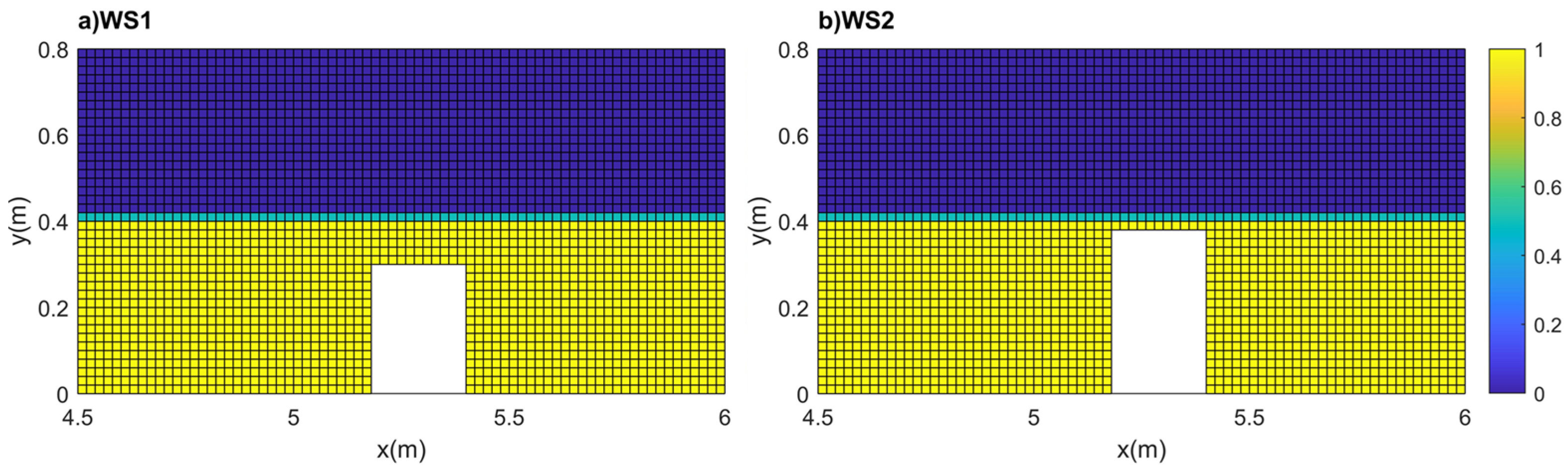
2.1. Basic Model Setups

We studied the behavior of microplastics in wavefields that interfered with underwater structures in the wave-dominant nearshore area using a CFD wave flume (ANSIS FLUENT 2020 R2). Figure 1 depicts the dimensions of a 12 m long and 0.8 m deep two-dimensional numerical wave flume. The still water depth (h) was set to 0.4 m, and the reference coordinate was set to the bottom left corner (x = 0 and y = 0), where x is the cross-shore coordinate pointing right, and y is the vertical coordinate pointing up. For observing the hydraulic properties downstream of the submerged structure, experiments were conducted with rectangular structures (Figure 2) of heights 0.3 m and 0.38 m, installed at x = 5 m (henceforth WS1 and WS2, respectively), and with no structure (henceforth NS). The mesh was built with a rectangular quadrilateral grid with a linear element order, and the grid size of 0.02 m established 24,560 (24,470) nodes and 23,850 (23,810) elements for the WS1 (WS2) case and 24,641 nodes and 24,000 elements for the NS case.

The PISO algorithm was utilized for pressure-velocity coupling with PRESTO, and compressive schemes were utilized to determine the pressure and volume fractions of a system. We also considered a second-order upwind scheme for the momentum, turbulent kinetic energy, specific dissipation rate, energy, and level-set function. We used a numerical time-step of 0.002 s for a total of 45,000 time-steps during the 90 s simulation for each run. The numerical solution at each time-step was found to converge by monitoring integrated quantities of bulk flow velocity and turbulence and scaled residuals of continuity, x, y velocity, energy, k-omega, and bulk water volume fraction.

2.2. Volume of Fluid and Wave Generation

We used the volume of fluid (VOF) model and open channel boundary conditions incorporated in ANSYS FLUENT to account for the water–air interaction in CFD wave flumes. The VOF model simulated multiphase fluids by solving a single set of momentum equations and monitoring the volume fraction of each fluid throughout the domain. We considered the standard laboratory environment such that two domains of air and water phases were created, with ambient densities of 1.225 and 998.2 $\mathrm{kg}/{\mathrm{m}}^3$, respectively. The air and water flow fields were computed by solving the unsteady Reynolds-averaged Navier–Stokes (URANS) equations with the shear stress transport (SST)–turbulent close model.

It was assumed that the submerged structure could retard the current and reduce the mass flow rate in the propagating direction, owing to the pressure drop induced by the structure. Therefore, rather than a fixed mass flow rate boundary condition, a pressure boundary condition with a constant velocity of 0.05 m/s and turbulence intensity of 5% was set at the inlet and outlet.

We aimed to simulate wave propagation in a shallow/intermediate-water wave field. Initial wave height (H) and wavelength (L) of 0.15 m and 1.5 m, respectively, were used at the inlet boundary, which made the ratio between nonlinearity and shallowness (Ursell number, H${\mathrm{L}}^2$/${\mathrm{h}}^3$) 5.27 and the ratio between inertial and gravitational forces (Froude number, $F_r$ = $\frac{V}{\sqrt{gy}}$) 0.025. Our wave field demonstrated a subcritical flow, with a faster wave propagation speed than the current speed. To emphasize the important nonlinear features in the dispersion of near-surface buoyant microplastics, we simulated wave propagation using Stokes’ 4th-order theory and estimated the free surface height ($\zeta$) as follows:

$$\zeta \left(X,t\right)=\frac{1}{k}{\displaystyle \sum }_{i=1}^{4 }{\displaystyle \sum }_{j=1}^{i }{b}_{ij}{\mathsf{\xi }}^i\cos \left(jk\left(x-ct\right)\right)$$

(1)

where $\xi =\pi H/2$, wave number $k=2\pi /L$, $c$ is the wave celerity, and $b_{ij}$ is the constant explained in Fenton (1990).

2.3. Microplastic Simulation by Discrete Phase Model

The discrete phase model (DPM) in ANSYS FLUENT was used to simulate microplastic behavior in shallow/intermediate wavefields in the nearshore area. The particle motion simulated by the DPM was characterized by the initial physical settings, such as particle size, shape, and density. We assumed that all microplastic particles were spherical and released particles of three different densities (900, 1000, and 1100 $\mathrm{kg}/{\mathrm{m}}^3$) and sizes (0.2, 1, and 5 mm). We simultaneously released 500 particles of varying densities and sizes near the surface at a height of 0.38 m (500 particles at x = 2, y = 0.38 m), 5 s after the simulations started. Microplastics are plastics with sizes ranging from 0.001 mm to 5 mm; however, in this experiment, only 0.2 mm, 1 mm, and 5 mm were used and labeled as small, medium, and large, respectively. Microplastics with densities of 900 and 1100 $\mathrm{kg}/{\mathrm{m}}^3$ were considered light and heavy particles, respectively.

The trajectory of a discrete phase particle was calculated by merging the force balance of the particle with that in a Lagrangian reference frame. The governing equations of Lagrangian inertial motion in ANSYS FLUENT were obtained from Morsi and Alexander (1972) [44]. According to the force balance equation, the particle inertia is equivalent to the force acting on the particle in the direction of motion and can be written as

$$\frac{d{u}_p}{dt}=F_D\left(u- u_p\right)+g\left(\frac{{\rho }_p – \rho }{{\rho }_p}\right)F_x$$

(2)

where $g$, $u$, and $\rho$ are the gravitational constant, velocity, and density, respectively. Parameters with the subscript $p$ are associated with the Lagrangian particle, and those without $p$ are associated with a Eulerian quantity at the particle location. $F_D\left(u- u_p\right)$ represents the drag force per unit particle mass, and $F_x$ represents the additional acceleration required to accelerate the fluid surrounding the particle and overcome the pressure gradient in the fluid. The drag force $F_D$ is calculated as $\frac{18\mu }{{\rho }_{p }{d}_p^2} \frac{C_D Re}{24}$, where $\mu$ is the fluid dynamic viscosity, $d_{p }$is the particle diameter, and $Re$ is the relative Reynolds number, defined as ${\rho }_{p }{d}_p\left|u- u_p\right|/\mu$. The drag coefficient ($C_D$) for spherical particles can be empirically fitted to the curve as follows:

$$C_{D }=k_{1 }+\frac{k_{2 }}{Re}+\frac{k_{3 }}{R{e}^2}$$

(3)

where $k_1$, $k_2$, and $k_3$, are the constants.

2.4. Numerical Simulation Case Study

This study simulated cases with and without the submerged structures (WS1 and WS2 for 0.3 and 0.38 m height structures, respectively, and NS for no structure) and no wave case for WS1 (WS1-nw). NS and WS1-nw imply an open-channel flow with and without a submerged structure, respectively. WS1 and WS2 imply flows where the intermediate waves propagate in the flow direction. The lowest wave depth (trough) was located above the structure (WS1) and below the structure (WS2). We characterized the effect of the submerged structure by comparing NS, WS1, and WS2 and that of the waves by comparing WS1 and WS1-nw. Based on the four Eulerian velocity fields (NS, WS1, WS2, and WS1-nw), microplastic particles with different densities (900, 1000, and 1100 $\mathrm{kg}/{\mathrm{m}}^3$) and sizes (0.2, 1, and 5 mm) were simulated. The 36 cases are summarized in

Table 1. Generated mesh properties.

Properties Meshing
Type Structure	Type Meshing/Method	Nodes	Elements	Average Surface Area $\left({\mathrm{m}}^2\right)$	Minimum Edge Length (m)	Element Order	Grid Size (m)
NS	Rectangular/ Quadrilaterals	24,641	24,000	9.6	0.8	Linear	0.02
WS1	Rectangular/ Quadrilaterals	24,506	23,850	9.54	0.2	Linear	0.02
WS2	Rectangular/ Quadrilaterals	24,470	23,810	9.52	0.2	Linear	0.02

.

3. Results

We describe our observations of the basic properties of the flow fields and particle behaviors. This section presents the velocity profiles and streamlines to investigate the Eulerian velocity fields for NS, WS1, and WS2 with the corresponding Lagrangian particle behaviors using ensemble-averaged particle trajectories.

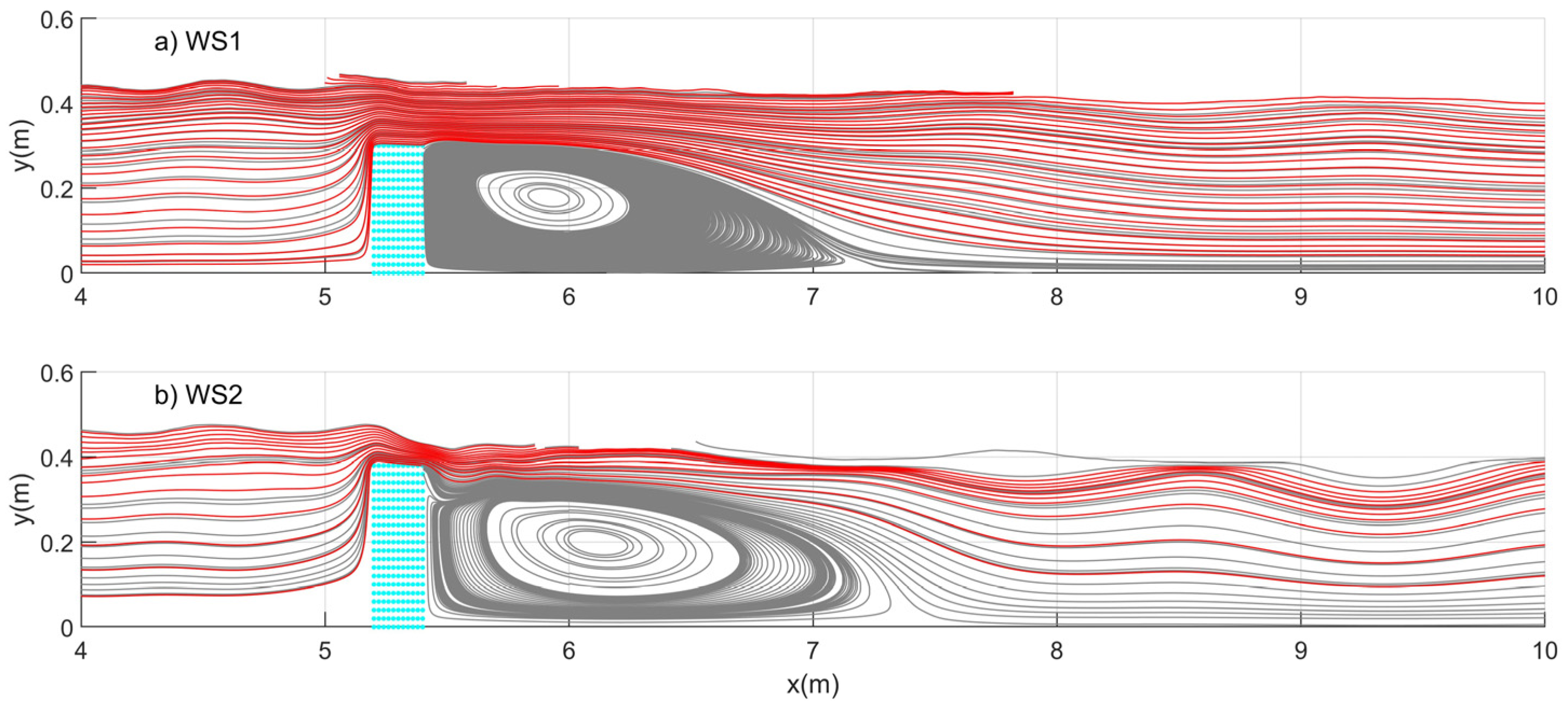
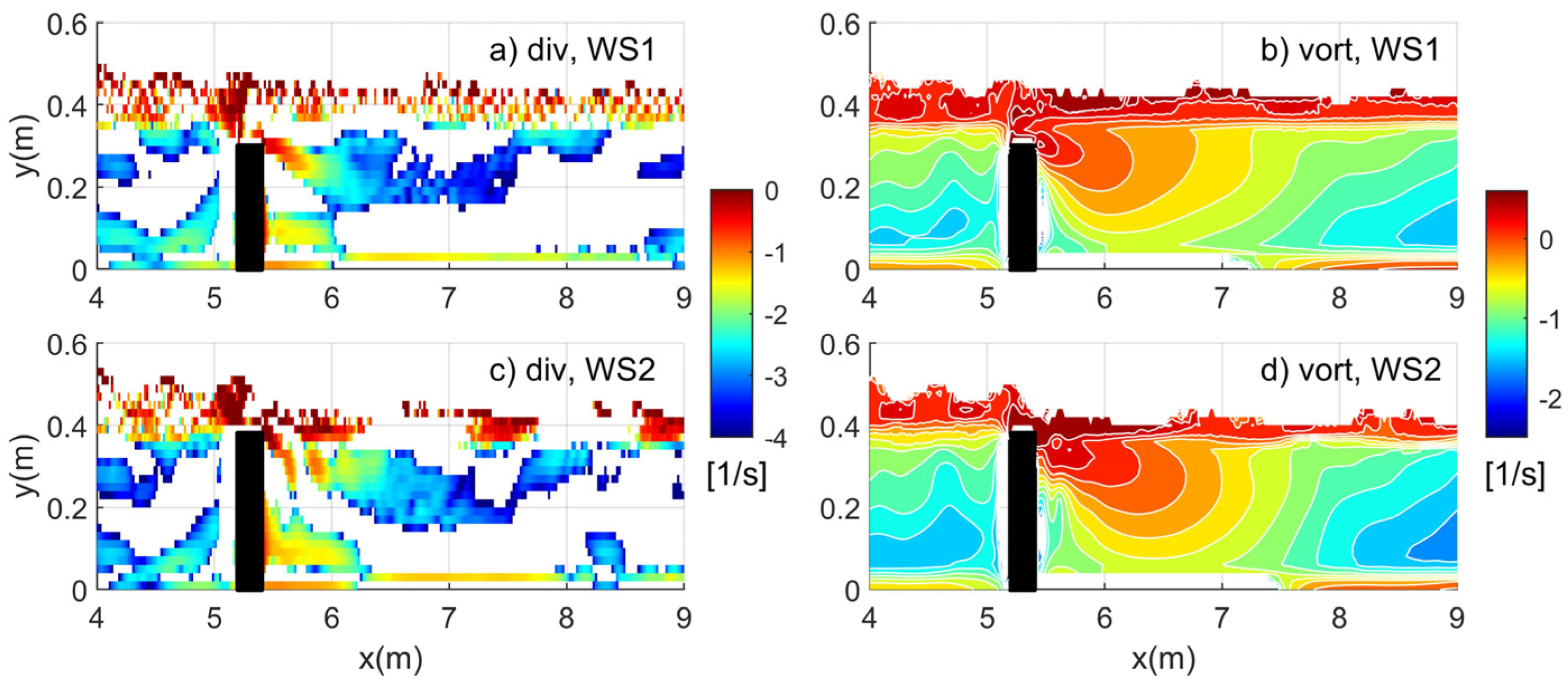
3.1. Eulerian Observations

Figure 3 shows the vertical velocity profiles at x locations. In the flow upstream of the submerged structure, NS and WS1 showed similar vertical velocity profiles, with the strong shear layer developed above h = 0.35 m. In contrast, WS2 exhibited a shear layer with a reduced magnitude above h = 0.4 m. At the passage, the maximum velocities of WS1 and WS2 were similar and approximately 1.5 times larger than those of NS. In the downstream, the maximum velocities of WS2 dominated from the passage to a distance of 1 m, but those of WS1 dominated the rest. Despite the same flow rate applied to NS, WS1, and WS2 inlets, the flow rate across the passage varied, given by $q_{NS}$ = 0.072 ${\mathrm{m}}^2/\mathrm{s}$, $q_{WS1}$ = 0.110 ${\mathrm{m}}^2/\mathrm{s}$, and $q_{WS2}$ = 0.098 ${\mathrm{m}}^2/\mathrm{s}$. Thus, the submerged structures experienced an increased flow rate at the passage. The backward movement of the orbit of particles flowing downstream through the structure was limited by upwelling, owing to recirculation and clogging of the structure. Moreover, WS1 had a slightly higher flow rate than WS2.

The streamlines of the mean velocity fields (Figure 4) showed that the submerged structure created a recirculation zone attached to structures of different heights. The increased structure height resulted in a slightly thicker and wider recirculation zone, with the reattachment points shifted downstream. There was little difference in the streamlines (marked in red) passing through the passage above the structure between WS1 and WS2. The WS1 streamlines scrubbed the bottom upstream, while the WS2 streamlines were disconnected from the bottom upstream, creating a hollow space below. Because the streamlines starting from the hollow space could pass through the wall, the residence time of microplastics in the lower upstream layer was able to be increased. The streamlines of WS2 also differed from those of WS1 in undulations, with a fixed phase near the surface beyond the recirculation region.

Figure 5 shows the Eulerian flow kinematics of the divergence ($=\partial \mathrm{u}/\partial \mathrm{x} +\partial \mathrm{v}/\partial \mathrm{y}$) and vorticity ($=\partial \mathrm{v}/\partial \mathrm{x} -\partial \mathrm{u}/\partial \mathrm{y}$) generated from the mean velocity fields. Strong convergence was observed on the left side of the wall (white region), where a strong dynamic pressure was applied. A similar strength of convergence was observed at the upper right end of the wall, above which a strong clockwise vorticity developed near the mainstream through the passage and at the lower right part of the wall, below which strong counter-clockwise vorticity was located at the bottom. The counter-clockwise (from wall to x = ~7.3 m) and clockwise (x = ~7.3 m) vorticities in the thin bottom layer can act similar to a conveyor belt and strongly affect the sinking particles near the bottom layer at x = 7.2 m (WS1) and 7.5 m (WS2), once they are entrained along the streamline.

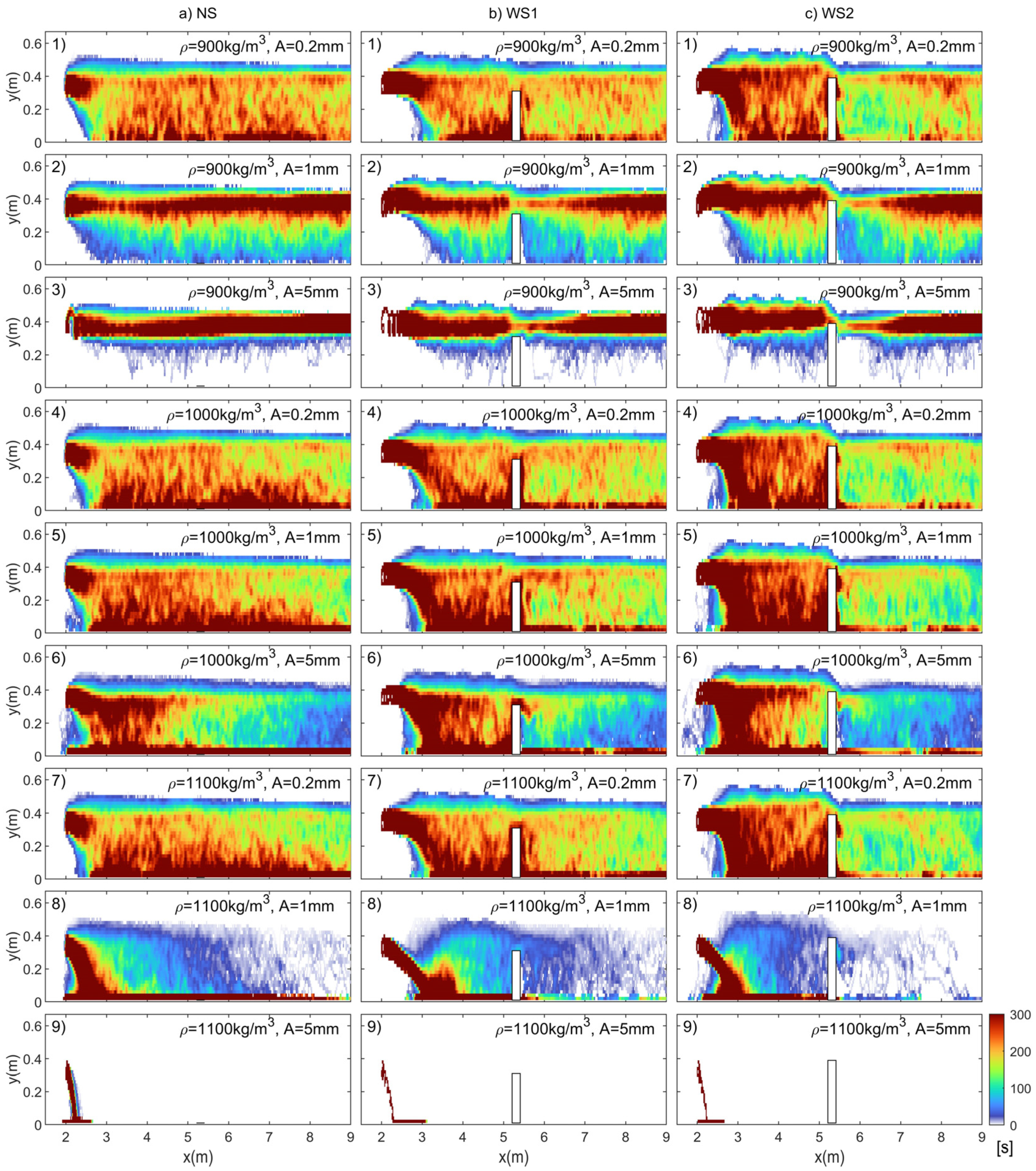
3.2. General Particle Behaviors

The instantaneous particle cloud in the experiments without any artificial submerged structures (NS) confirmed that the mixture of microplastics was dispersed and sorted by particle size and density. The large low-density particles near the surface were advected in the direction of wave propagation, owing to the mean surface current induced by the waves. However, the large high-density particles entrained into the bottom layer near the no-slip boundary were hardly resuspended but oscillated in the horizontal direction with a small amplitude.

In contrast, the smaller particles quickly occupied the vertical domain, regardless of their density. The vertical shear induced by the weak and strong flow speeds in the lower and upper layers, respectively, effectively stretched the particle cloud in the horizontal direction. Thus, for low-density particles, the smaller the particles, the stronger the horizontal dispersion of the particle cloud, but the larger the particles, the stronger the horizontal displacement. For high-density particles, the larger the particles, the weaker the horizontal advection because the particles remained near the bottom of the slowest flow speed, whereas the smaller the particles, the stronger the horizontal dispersion, as observed in the low-density particles. This will be discussed in more detail in Section 4.

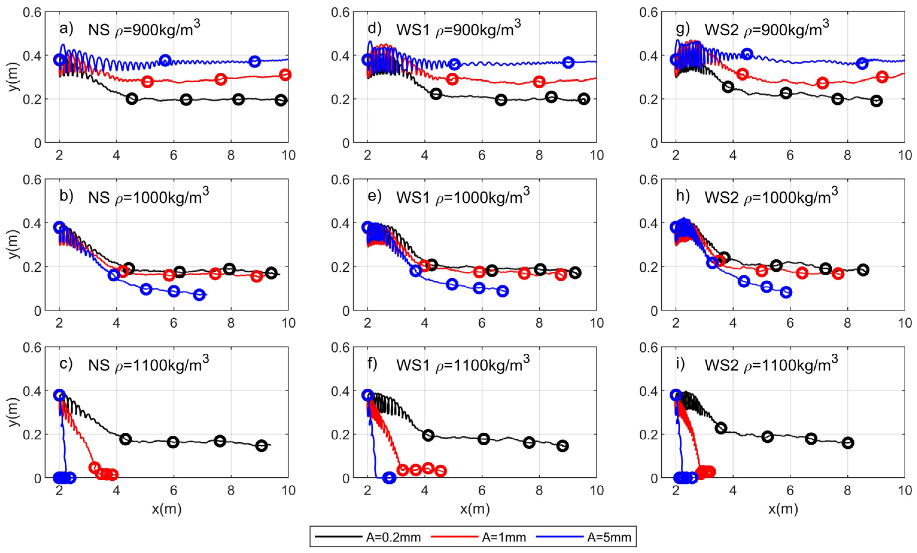
3.3. Mean Particle Trajectories

The mean trajectories of the 500 particles released near the surface at (x, y) = (2, 0.38) m demonstrated a strong dependency of particle size and density on the mean displacemen (Figure 6). The mean vertical displacement of low-density particles decreased with increasing particle size. In contrast, the displacement of the high-density particles moved closer to the bottom with increasing particle size, as expected. For small particle sizes, the mean displacement displayed no significant differences, remaining at a depth of nearly 0.2 m for all density cases. The mean horizontal displacement significantly changed with particle density. For low-density particles, the mean horizontal displacement upstream (downstream) was the greatest in the case of NS (WS1), but for heavy particles, the greatest displacement upstream and downstream was observed in NS. The effect of installing a submerged structure increased slightly as the particle size and density increased. Hence, the small- and low-density particle cases showed no perceptible difference between the cases with and without the structure. The change in height from 0.3 m (WS1) to 0.38 m (WS2) did not affect the mean trajectories. However, the taller submerged structure (WS2) showed a slightly slower flow speed, resulting in a final horizontal displacement approximately 1 m shorter than that of WS1.

4. Discussion

We discuss the distribution, accumulation, and dispersion of microplastics based on the Eulerian flow kinematics and the particle statistics of residence time and relative dispersion.

4.1. Microplastic Accumulation

The region of strong clockwise vorticity and the divergent region coincided with the upper part of the large vortex (or recirculation zone), acting as a filter that sends only small-sized or denser particles to the recirculation region. Likewise, the strong counter-clockwise vortex and convergent region coincided with the lower part of the vortex, acting as a collector to store heavier particles. Convergence and divergence were scattered on the surface of WS1 but were separated on the downstream surface of WS2. The periodic pattern of convergence and divergence was well-represented in the streamlined undulation with a fixed phase from the wall (Figure 4). However, this experiment did not observe the accumulation of particles in the convergence regions because of the mean current moving in the x-direction.

The residence time ${\mathrm{t}}_{\mathrm{r}}$ in Figure 7 shows the Lagrangian accumulation and distribution of microplastic particles that are strongly dependent on particle size and density. Each column displays the residence time map for NS, WS1, and WS2. Each column includes nine cases of various particle sizes and densities. Small particles were more evenly distributed than others and were more pronounced near boundaries, such as surfaces, floors, and structures, as shown in Figure 7((1),(4),(7)). Although small light particles are accumulated near the surface in nature, the wave-induced perturbations in the upper layer introduced the particles into the bottom boundary layers, where a small, wave-induced flat motion prolonged the residence time.

For the medium and large-sized small particles (Figure 7((2),(3))), the particles were most frequently present near the still water level, except for the water passage downstream, where the strong clockwise vortex swiftly transported the particles into various depths of the water column. Because the medium and large particles had sufficient buoyancy to overcome the gravitational force, they were not engaged in the clockwise vortex to be recirculated but floated and proceeded in the forward direction.

The differences in accumulation after installing a structure are quantified by the residence time ratio $\mathsf{\tau } ={ \mathrm{t}}_{\mathrm{r},\mathrm{d}}/{\mathrm{t}}_{\mathrm{r},\mathrm{u}}$, as tabulated in

Table 2. Residence time ratio ($\mathsf{\tau } ={ \mathrm{t}}_{\mathrm{r},\mathrm{d}}/{\mathrm{t}}_{\mathrm{r},\mathrm{u}}$ ).

$$\mathit{\rho }\left(\mathbf{k}\mathbf{g}/{\mathbf{m}}^3\right)$$	A (mm)	NS	WS1	WS2
900	0.2	1.64	1.49 (0.91)	1.00 (0.61)
900	1	2.33	2.02 (0.87)	1.60 (0.69)
900	5	2.62	1.89 (0.72)	1.81 (0.69)
1000	0.2	1.47	1.32 (0.90)	0.85 (0.58)
1000	1	1.21	1.05 (0.87)	0.62 (0.51)
1000	5	0.62	0.49 (0.78)	0.30 (0.49)
1100	0.2	1.32	1.18 (0.89)	0.69 (0.52)
1100	1	0.13	0.07 (0.61)	0.01 (0.12)
1100	5	-	-	-

${\mathrm{t}}_{\mathrm{r},\mathrm{u}}$ and ${\mathrm{t}}_{\mathrm{r},\mathrm{d}}$ indicate the summation of residence time upstream and downstream, respectively. The numbers in the parenthesis are normalized values by the NS value. The lower the value, the greater the influence of the artificial structure. The last row cannot be obtained, due to there being no particle downstream of the structure.

, where ${\mathrm{t}}_{\mathrm{r},\mathrm{d}}$ and ${\mathrm{t}}_{\mathrm{r},\mathrm{u}}$ are the spatial sum of residence time measured downstream and upstream, respectively. This ratio evaluates the change in accumulation between the two regions separated by the structure; a larger ratio represents a longer residence time in the downstream flow. In all cases, the reduction in $\mathsf{\tau }$ increased as the particle density increased, demonstrating that the impact of installing the submerged structure on the accumulation increased with particle density (e.g., Figure 7(a(7)) vs. Figure 7(c(7))). The biggest impact was observed when the particle size and density were 1 mm and 1100 $\mathrm{kg}/{\mathrm{m}}^3$, respectively (Figure 7(8) and Table 2), which is possibly explained by the strength of resuspension: the smaller particles (0.2 mm and 1100 $\mathrm{kg}/{\mathrm{m}}^3$) were easily resuspended, crossing over downstream (Figure 7(7)), while the large particles (5 mm and 1100 $\mathrm{kg}/{\mathrm{m}}^3$) were hardly resuspended and remained upstream. Therefore, the largest reduction in τ, or the highest impact by installing structures, was observed for intermittently resuspended particles.

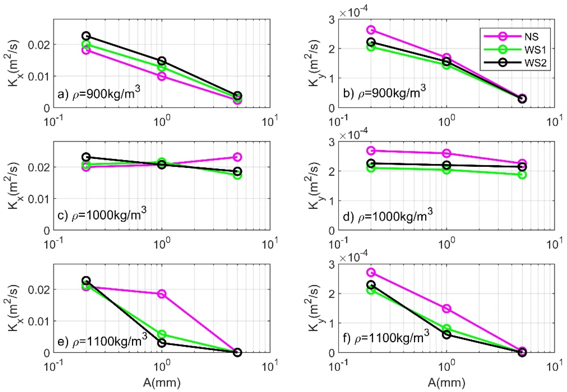
4.2. Microplastic Dispersion

The strength of particle dispersion in the horizontal and vertical directions was quantified by the relative dispersion coefficient calculated as $\mathrm{K}\left(\mathrm{t}\right)=\frac{<\sigma {\left(t\right)}^2>}{4t}$, where $\sigma {\left(t\right)}^2$ is the variance of distances between two particles, <> indicates an ensemble average, and $t$ is the elapsed time [45]. Because this metric measures the distance between two particles, it can be considered the strength of the particle spread. The averaged relative dispersion coefficient ${\mathrm{K}}_{\mathrm{y}}$ (Figure 8b,d,f) shows that smaller particles resulted in a stronger dispersion in the vertical direction. For low-density particles, the large-size particles dispersed less because they remained near the surface, owing to the strong buoyancy, and the small particles dispersed more because they were easily entrained into the deep, owing to the weak buoyancy and wave-induced unclosed orbital motions. Similarly, for the heavy, dense particles, the large-sized particles dispersed less because they remained near the bottom, owing to the strong gravitational force, and the small-sized particles dispersed more because they were easily resuspended into the depths, owing to the weak gravitational force.

The averaged relative dispersion coefficient ${\mathrm{K}}_{\mathrm{x}}$ (Figure 8a,c,e) shows that the smaller particles resulted in a stronger dispersion in the horizontal direction, associated with the strong vertical dispersion of the small particles. The shear flow dispersion can explain this mechanism: the stronger the vertical mixing, the stronger the horizontal dispersion in a bounded flow [46,47,48]. Because the intermediate waves (h/L = 0.27) propagated on a relatively shallow depth flow, the particles released at the surface had an increased probability of reaching the bottom boundary in a short time. Once the vertical distribution of particle concentration became saturated, the horizontal dispersion coefficient was linearly proportional to the vertical dispersion coefficient. In our application, the small particles quickly occupied the vertical domain, and the strong vertical shear developed by the slow mean currents near the bottom and the fast mean currents near the surface effectively elongated the particle cloud in the horizontal direction.

Installing a submerged structure can enhance the horizontal spreading of low-density particles (Figure 8a) but limits the horizontal spreading of high-density particles (Figure 8e). The largest difference between the NS and WS cases was found for heavy- and medium-sized particles ($\mathsf{\rho }$ = 1100 $\mathrm{kg}/{\mathrm{m}}^3$ and A = 1 mm in Figure 8e), at which the ${\mathrm{K}}_{\mathrm{x}}$ for NS was approximately four times larger than the ${\mathrm{K}}_{\mathrm{x}}$ for WS cases. The heavy, medium-sized particles settled slowly, owing to the shear dispersion mechanism, and once they reached the bottom, resuspension occurred relatively frequently and advanced intermittently. However, when the structure was met, heavy, medium-sized particles could not pass the structure. This large difference in ${\mathrm{K}}_{\mathrm{x}}$ did not occur for heavy small- and large-sized particles because most particles, in the absence of a structure, swam freely in water regardless of the walls, whereas most particles were stuck to the bottom without any resuspension when structures were included.

5. Conclusions

The results revealed that the particle size and density influence the particle behavior around the artificial structure. Small particles (0.2 mm) showed a high dispersion rate and were more evenly distributed, regardless of the particle density. Moreover, the effect of installing the structure increased slightly with increasing particle density. The enhanced dispersion of the cloud consisting of small-sized particles can be explained by shear flow dispersion. Owing to the small timescale of vertical mixing in shallow waters, the gradient of the vertical particle distribution was rapidly degraded. In turn, the vertical distribution was elongated by the strong shear and was continuously saturated by vertical mixing. The heavy (1100 $\mathrm{kg}/{\mathrm{m}}^3$) and large (5 mm) particles showed the weakest horizontal dispersion rate and no transportation through the structure because no resuspension occurred once they sank to the bottom; therefore, the effect of installing the submerged structure was negligible. The heavy (1100 $\mathrm{kg}/{\mathrm{m}}^3$) and medium-sized (1 mm) particles showed augmented horizontal dispersion because resuspension occurred for those particles, allowing some of the particles to pass over the structure, so the effect of installing the structure was maximized.

These results suggest that the fate of microplastics adjacent to artificial reefs in coastal areas may vary depending on the physical properties of microplastics. Therefore, microplastic concentrations are made selectively by regions, emphasizing the need for diversifying collection strategies. Because artificial reefs are designed to restore degraded habitats, the structures attracting the biomass can accelerate the consumption of microplastics in fish and small organisms. Our result can be used to formulate more specific strategies regarding collection locations and methods near the artificial structures by providing the characteristics of the Eulerian flow fields and the corresponding Lagrangian particle behaviors.

This study is limited to the behavior of large microplastics in a two-dimensional idealized environment with intermediate waves near a very simple shape of artificial structure. Because we only considered microplastics with spherical shapes, further research is urgently required to consider the behavior of microplastics with various shapes, such as fibers and fragments, with appropriate corresponding drag coefficients. Furthermore, CFD- and laboratory-based research with more realistic environments, including bottom slopes, wind-induced mixing, the shape of artificial reefs, particle properties, and various mean currents, are required to establish a robust collection strategy of microplastics near submerged artificial structures.

References

1. Koelmans Albert, A.; Redondo-Hasselerharm, P.E.; Nor, N.H.; de Ruijter, V.N.; Mintenig, S.M.; Kooi, M. Risk assessment of microplastic particles. Nat. Rev. Mater. 2022, 7, 138–152. [Google Scholar] [CrossRef]
2. Li, C.; Zhu, L.; Wang, X.; Liu, K.; Li, D. Cross-oceanic distribution and origin of microplastics in the subsurface water of the South China Sea and Eastern Indian Ocean. Sci. Total Environ. 2022, 805, 150243. [Google Scholar] [CrossRef] [PubMed]
3. Tien, C.-J.; Wang, Z.-X.; Colin, S.C. Microplastics in water, sediment and fish from the Fengshan River system: Relationship to aquatic factors and accumulation of polycyclic aromatic hydrocarbons by fish. Environ. Pollut. 2020, 265, 114962. [Google Scholar] [CrossRef]
4. Abeynayaka, A.; Kojima, F.; Miwa, Y.; Ito, N.; Nihei, Y.; Fukunaga, Y.; Yashima, Y.; Itsubo, N. Rapid sampling of suspended and floating microplastics in challenging riverine and coastal water environments in Japan. Water 2020, 12, 1903. [Google Scholar] [CrossRef]
5. Crawford, C.B.; Quinn, B. 5-Microplastics, standardisation and spatial distribution. In Microplastic Pollutants; Elsevier: Amsterdam, The Netherlands, 2017; pp. 101–130. [Google Scholar]
6. Law, K.L. Plastics in the marine environment. Annu. Rev. Mar. Sci. 2017, 9, 205–229. [Google Scholar] [CrossRef] [Green Version]
7. McAfee, D.; Connell, S.D. The global fall and rise of oyster reefs. Front. Ecol. Environ. 2021, 19, 118–125. [Google Scholar] [CrossRef]
8. Caputo, F.; Vogel, R.; Savage, J.; Vella, G.; Law, A.; Della Camera, G.; Hannon, G.; Peacock, B.; Mehn, D.; Ponti, J.; et al. Measuring particle size distribution and mass concentration of nanoplastics and microplastics: Addressing some analytical challenges in the sub-micron size range. J. Colloid Interface Sci. 2021, 588, 401–417. [Google Scholar] [CrossRef] [PubMed]
9. de Paiva JN, S.; Walles, B.; Ysebaert, T.; Bouma, T.J. Understanding the conditionality of ecosystem services: The effect of tidal flat morphology and oyster reef characteristics on sediment stabilization by oyster reefs. Ecol. Eng. 2018, 112, 89–95. [Google Scholar] [CrossRef]
10. Shnada, A.H.; Emenike, C.U.; Fauziah, S.H. Distribution and importance of microplastics in the marine environment: A review of the sources, fate, effects, and potential solutions. Environ. Int. 2017, 102, 165–176. [Google Scholar]
11. Chubarenko, I.; Esiukova, E.; Bagaev, A.; Isachenko, I.; Demchenko, N.; Zobkov, M.; Efimova, I.; Bagaeva, M.; Khatmullina, L. Behavior of microplastics in coastal zones. In Microplastic Contamination in Aquatic Environments; Elsevier: Amsterdam, The Netherlands, 2018; pp. 175–223. [Google Scholar]
12. Rezania, S.; Park, J.; Din, M.F.; Taib, S.M.; Talaiekhozani, A.; Yadav, K.K.; Kamyab, H. Microplastics pollution in different aquatic environments and biota: A review of recent studies. Mar. Pollut. Bull. 2018, 133, 191–208. [Google Scholar] [CrossRef]
13. Savoca, S.; Bottari, T.; Fazio, E.; Bonsignore, M.; Mancuso, M.; Luna, G.M.; Romeo, T.; D’Urso, L.; Capillo, G.; Panarello, G.; et al. Plastics occurrence in juveniles of Engraulis encrasicolus and Sardina pilchardus in the Southern Tyrrhenian Sea. Sci. Total Environ. 2020, 718, 137457. [Google Scholar] [CrossRef] [PubMed]
14. Savoca, M.S.; McInturf, A.G.; Hazen, E.L. Plastic ingestion by marine fish is widespread and increasing. Glob. Chang. Biol. 2021, 27, 2188–2199. [Google Scholar] [CrossRef] [PubMed]
15. Yuan, Z.; Nag, R.; Cummins, E. Human health concerns regarding microplastics in the aquatic environment-From marine to food systems. Sci. Total Environ. 2022, 823, 153730. [Google Scholar] [CrossRef]
16. Han, Z.; Jiang, T.; Xie, L.; Zhang, R. Microplastics impact shell and pearl biomineralization of the pearl oyster Pinctada fucata. Environ. Pollut. 2022, 293, 118522. [Google Scholar] [CrossRef] [PubMed]
17. Heemink, A.W. Stochastic modelling of dispersion in shallow water. Stoch. Hydrol. Hydraul. 1990, 4, 161–174. [Google Scholar] [CrossRef] [Green Version]
18. Spagnol, S.; Wolanski, E.; Deleersnijder, E.; Brinkman, R.; McAllister, F.; Cushman-Roisin, B.; Hanert, E. An error frequently made in the evaluation of advective transport in two-dimensional Lagrangian models of advection-diffusion in coral reef waters. Mar. Ecol. Prog. Ser. 2002, 235, 299–302. [Google Scholar] [CrossRef] [Green Version]
19. Deleersnijder, E. A Depth-Integrated Diffusion Problem in a Depth-Varying, Unbounded Domain for Assessing Lagrangian Schemes. In Technical Report; Université Catholique de Louvain: Ottignies-Louvain-la-Neuve, Belgium, 2015. [Google Scholar]
20. Critchell, K.; Lambrechts, J. Modelling accumulation of marine plastics in the coastal zone; what are the dominant physical processes? Estuar. Coast. Shelf Sci. 2016, 171, 111–122. [Google Scholar] [CrossRef]
21. van Bergeijk, V.; Warmink, J.; Frankena, M.; Hulscher, S. Modelling dike cover erosion by overtopping waves: The effects of transitions. Coast. Struct. 2019, 2019, 1097–1106. [Google Scholar]
22. Camins, E.; de Haan, W.P.; Salvo, V.S.; Canals, M.; Raffard, A.; Sanchez-Vidal, A. Paddle surfing for science on microplastic pollution. Sci. Total Environ. 2020, 709, 136178. [Google Scholar] [CrossRef]
23. Barrientos, E.E.; Paris, A.; Rohindra, D.; Rico, C. Presence and abundance of microplastics in edible freshwater mussel (Batissa violacea) on Fiji’s main island of Viti Levu. Mar. Freshw. Res. 2022, 73, 528–539. [Google Scholar] [CrossRef]
24. Wu, Z.; Tweedley, J.R.; Loneragan, N.R.; Zhang, X. Artificial reefs can mimic natural habitats for fish and macroinvertebrates in temperate coastal waters of the Yellow Sea. Ecol. Eng. 2019, 139, 105579. [Google Scholar] [CrossRef]
25. Ding, Y.; Liu, H.; Yu, D.; Song, J.; Duan, G. The migration of viscous fish eggs in artificial reefs. Ecol. Model. 2022, 469, 109985. [Google Scholar] [CrossRef]
26. Zheng, Y.; Kuang, C.; Zhang, J.; Gu, J.; Chen, K.; Liu, X. Current and turbulence characteristics of perforated box-type artificial reefs in a constant water depth. Ocean Eng. 2022, 244, 110359. [Google Scholar] [CrossRef]
27. Walles, B.; Troost, K.; van den Ende, D.; Nieuwhof, S.; Smaal, A.C.; Ysebaert, T. From artificial structures to self-sustaining oyster reefs. J. Sea Res. 2016, 108, 1–9. [Google Scholar] [CrossRef]
28. Allan, R.P.; Hawkins, E.; Bellouin, N.; Collins, B. Summary for Policymakers. IPCC 2021, 2021, 3–32. [Google Scholar]
29. Tebaldi, C.; Ranasinghe, R.; Vousdoukas, M.; Rasmussen, D.J.; Vega-Westhoff, B.; Kirezci, E.; Kopp, R.E.; Sriver, R.; Mentaschi, L. Extreme sea levels at different global warming levels. Nat. Clim. Chang. 2021, 11, 746–751. [Google Scholar] [CrossRef]
30. Chowdhury, M.S.N. Ecological Engineering with Oysters for Coastal Resilience: Habitat Suitability, Bioenergetics, and Ecosystem Services. Ph.D. Thesis, Wageningen University and Research, Wageningen, The Netherlands, 2019. [Google Scholar]
31. Wang, X.; Feng, J.; Lin, C.; Liu, H.; Chen, M.; Zhang, Y. Structural and Functional Improvements of Coastal Ecosystem Based on Artificial Oyster Reef Construction in the Bohai Sea, China. Front. Mar. Sci. 2022, 9, 829557. [Google Scholar] [CrossRef]
32. Fodrie, F.J.; Rodriguez, A.B.; Gittman, R.K.; Grabowski, J.H.; Lindquist, N.L.; Peterson, C.H.; Piehler, M.F.; Ridge, J.T. Oyster reefs as carbon sources and sinks. Proc. R. Soc. B Biol. Sci. 2017, 284, 20170891. [Google Scholar] [CrossRef] [Green Version]
33. Kim, D.; Woo, J.; Yoon, H.S.; Na, W.B. Wake lengths and structural responses of Korean general artificial reefs. Ocean Eng. 2014, 92, 83–91. [Google Scholar] [CrossRef]
34. Van Sebille, E.; Wilcox, C.; Lebreton, L.; Maximenko, N.; Hardesty, B.D.; Van Franeker, J.A.; Eriksen, M.; Siegel, D.; Galgani, F.; Law, K.L. A global inventory of small floating plastic debris. Environ. Res. Lett. 2015, 10, 124006. [Google Scholar] [CrossRef]
35. Morteza, A.; Passandideh-Fard, M.; Moghiman, M. Fully nonlinear viscous wave generation in numerical wave tanks. Ocean Eng. 2013, 59, 73–85. [Google Scholar]
36. Alsina, J.M.; Jongedijk, C.E.; van Sebille, E. Laboratory Measurements of the Wave-Induced Motion of Plastic Particles: Influence of Wave Period, Plastic Size and Plastic Density. J. Geophys. Res. Ocean. 2020, 125, e2020JC016294. [Google Scholar] [CrossRef]
37. Eldeen AS, S.; El-Baz, A.M.; Elmarhomy, A.M. CFD Modeling of Regular and Irregular Waves Generated by Flap Type WaveMaker. J. Adv. Res. Fluid Mech. Therm. Sci. 2021, 85, 128–144. [Google Scholar] [CrossRef]
38. Ma, Y.; Yuan, C.; Ai, C.; Dong, G. Comparison between a non-hydrostatic model and OpenFOAM for 2D wave-structure interactions. Ocean Eng. 2019, 183, 419–425. [Google Scholar] [CrossRef]
39. Miquel, A.M.; Kamath, A.; Alagan Chella, M.; Archetti, R.; Bihs, H. Analysis of different methods for wave generation and absorption in a CFD-based numerical wave tank. J. Mar. Sci. Eng. 2018, 6, 73. [Google Scholar] [CrossRef] [Green Version]
40. Hu, Z.Z.; Greaves, D.; Raby, A. Numerical wave tank study of extreme waves and wave-structure interaction using OpenFoam®. Ocean Eng. 2016, 126, 329–342. [Google Scholar] [CrossRef] [Green Version]
41. Wu, G.; Oakley, O.H., Jr. CFD modeling of fully nonlinear water wave tank. In Proceedings of the International Conference on Offshore Mechanics and Arctic Engineering, Honolulu, HI, USA, 31 May–5 June 2009; ASME: New York, NY, USA, 2019; Volume 43451, pp. 815–823. [Google Scholar]
42. Fatahi, M.; Akdogan, G.; Dorfling, C.; Van Wyk, P. Numerical Study of Microplastic Dispersal in Simulated Coastal Waters Using CFD Approach. Water 2021, 13, 3432. [Google Scholar] [CrossRef]
43. Ahmadi, P.; Elagami, H.; Dichgans, F.; Schmidt, C.; Gilfedder, B.S.; Frei, S.; Peiffer, S.; Fleckenstein, J.H. Systematic Evaluation of Physical Parameters affecting the Terminal Settling Velocity of Microplastic Particles in Lakes using CFD. Front. Environ. Sci. 2022, 10, 389. [Google Scholar] [CrossRef]
44. Morsi, S.A.J.; Alexander, A.J. An investigation of particle trajectories in two-phase flow systems. J. Fluid Mech. 1972, 55, 193–208. [Google Scholar] [CrossRef]
45. Okubo, A. Oceanic diffusion diagrams. In Deep Sea Research and Oceanographic Abstracts; Elsevier: Amsterdam, The Netherlands, 1971; Volume 18, pp. 789–802. [Google Scholar]
46. Choi, J.; Troy, C.; Hawley, N.; McCormick, M.; Wells, M. Lateral dispersion of dye and drifters in the center of a very large lake. Limnol. Oceanogr. 2020, 65, 336–348. [Google Scholar] [CrossRef]
47. Sundermeyer, M.A.; Ledwell, J.R. Lateral dispersion over the continental shelf: Analysis of dye release experiments. J. Geophys. Res. Ocean. 2001, 106, 9603–9621. [Google Scholar] [CrossRef]
48. Taylor, G.I. Diffusion by continuous movements. Proc. Lond. Math. Soc. 1922, 2, 196–212. [Google Scholar] [CrossRef]
Figure 1. Schematic of computational fluid dynamics (CFD) wave flume (A: wavemaker, B: artificial reef, H: wave height, h: still water, L: wavelength, η: free surface, d: height of artificial reef, l: length of artificial reef, yellow and red circle: release locations of microplastics). The origin is located at the bottom left corner.
Jmse 10 01934 g001
Figure 2. Grid meshing for WS1 (a) and WS2 (b).
Jmse 10 01934 g002
Figure 3. (a) Vertical velocity profiles calculated by the mean velocity fields for NS, WS1, and WS2. (b) Displays enlarged (a). The 0.5 m in the x-axis can be scaled as 1.43 m/s of velocity profiles.
Jmse 10 01934 g003
Figure 4. Streamlines for (a) WS1 and (b) WS2. The gray lines indicate streamlines that pass through the points, with 0.025 m spacings at vertical lines at x = 5.46 (just beside the structure), 6 (center of the recirculation zone), and 7.7 m (end of the recirculation zone). The red lines indicate streamlines that pass through the points at the passage above the submerged structure.
Jmse 10 01934 g004
Figure 5. Divergence (a,c) and clockwise vorticity (b,d) in log scale for WS1 and WS2. The submerged structure is marked as black bars. The region of convergence in (a,c) and the counter-clockwise vorticity in (b,d) has no color. The legends indicate the log of divergence and convergence.
Jmse 10 01934 g005
Figure 6. Mean trajectories of 500 particles released at (x, y) = (2, 0.38) m. The circles indicate the mean locations every 20 s.
Jmse 10 01934 g006
Figure 7. Residence time t r in seconds accumulated at each grid cell for all particles during simulation time. x- and y-axes are the distances from the origin shown in Figure 1.
Jmse 10 01934 g007
Figure 8. Relative dispersion coefficients K in the horizontal direction (a,c,e) and in the vertical direction (b,d,f) depending on particle size A in the log scale.
Jmse 10 01934 g008