Properties of the Acoustic Vector Field near the Underwater Planar Cavity Baffle and Its Application

Abstract

In order to apply the acoustic vector hydrophone on a ship, the properties of the acoustic vector field near the underwater planar cavity baffle are studied based on the Euler description and Lagrange description. The acoustic vector field is calculated based on the transfer matrices and matched boundary conditions. It is shown that the interference structure appears in the acoustic field. In particular, the particle velocity direction and intensity vector cannot directly reflect the azimuth of the source. The points at which the particle velocity is zero are saddle points and nodal points in the particle velocity vector field. Moreover, the particle motion is generally an ellipse near the planar cavity baffle. Furthermore, this paper defines a parameter that can fully represent the particle motion, and the direction of arrival (DOA) can be estimated using a single acoustic vector hydrophone using this parameter in some cases. At the end, the validity of the theoretical calculation and the method of using the parameter to estimate the DOA are verified experimentally.

1. Introduction

An acoustic vector hydrophone can simultaneously acquire the pressure and two or three orthogonal components of the particle velocity at one point in the marine environment. The acoustic vector hydrophone has been utilized in many applications such as geoacoustic inversion [1], underwater acoustic communications [2], pipeline [3], and source localization [4,5,6,7]. Many scholars have done a great deal of research related to the DOA estimation, and the results show that acoustic vector hydrophones have advantages in the estimation and give rise to an improved resolution by using the particle velocity information [4,5,6,7]. However, most of these studies have only considered acoustic vector hydrophones used in free space. When the sonar system is mounted on a ship, the acoustic field will no longer meet the free-space assumption due to the influence of acoustic baffle, so the results of the researches in the free space are no longer applicable. Therefore, the application of the acoustic vector hydrophone in the presence of the baffle has become a critical problem.

The research on acoustic vector field with consideration of the acoustic hydrophone carrier is the basis of the application of acoustic vector hydrophone mounted on a ship. Many scholars have been involved in related studies. Kosobrodov et al. [8] studied the acoustic properties near the solid spherical shell in finite space and the influence on vector hydrophone. Barton et al. [9] calculated the acoustic pressure distribution near the rigid spheroid with an arbitrary incident acoustic field. Ji et al. [10] discussed the influences of the prolate spheroidal baffle on the directivity of an acoustic vector hydrophone. Roumeliotis et al. [11] calculated the sound diffraction of a plane wave from an impenetrable, soft or hard, and prolate or oblate spheroid. In addition, some scholars studied the acoustic intensity field; the results indicate that the acoustic intensity is always complex in the acoustic field due to the influence of the acoustic vector hydrophone carrier [12,13]. In these cases, the acoustic intensity field is characterized by both active and reactive intensity, as the phases of the pressure and the particle velocity are not necessarily the same. Mann et al. [14] demonstrated the propagation of energy and the distinction between energy propagation and wave front propagation in an acoustic field where the reactive intensity is nonzero. Several scholars have also studied the particle velocity vector field near the acoustic baffle in detail. Moreover, some scholars have considered the signal processing in the presence of a reflecting boundary. Hawkes [15] and Javad et al. [16] studied the DOA estimation using acoustic vector hydrophone arrays in this case and derived an expression for the Cramér–Rao bound (CRB). However, there is no method aimed at using a single acoustic-vector hydrophone to estimate DOA in the presence of baffle.

The particle motion associated with the propagation of sound is also one of the fundamental properties, as well as pressure, particle velocity, and acoustic intensity. In an acoustic field with harmonic time dependence, the trajectory of particles in a small parcel of fluid, defined here as having a characteristic scale much less than acoustic wavelength, will be uniform and will repeat once every period [17]. Additional vector information can be obtained from the phase relationship between the components of the particle velocity. If the components of particle velocity are in phase, the acoustic particle motion trajectory in the corresponding plane will be a straight line. If the components of particle velocity are out of phase, the acoustic particle motion trajectory will be an ellipse. The elliptical motion can occur in acoustic fields characterized by multi-path interference [17,18,19,20,21]. Campbell et al. studied the particle motion in the fish tank to analyze the acoustic sensitivity of fish [18]. Dall’Osto et al. [17,19,20] measured and discussed the particle motion in the waveguide and applied it to geoacoustic inversion. Osler et al. [21] measured and modeled the seabed particle motion using buried vector sensors. However, to the best of our knowledge, the acoustic particle motion near the acoustic baffle is not yet studied and applied to the following signal processing.

The planar cavity baffle is a kind of baffle that can reduce the structure vibration and noise in the hull-mounted sonar system. In this paper, the properties of the acoustic vector field near the underwater planar cavity baffle are analyzed. The baffle used in the flank array is long enough to be simplified to an infinite planar multilayer structure, so the acoustic vector field near the planar cavity baffle can be obtained based on the transfer matrices and matched boundary conditions [22,23,24,25]. The properties of pressure, particle velocity vector, and complex intensity are analyzed in detail. In particular, the acoustic particle motion near the baffle is discussed. Additionally, this paper presents a method to estimate the DOA using a single acoustic vector hydrophone based on the properties of the acoustic vector field near the baffle. In addition, an experiment applying a single acoustic-vector hydrophone near the underwater planar cavity baffle is carried out.

2. The Method of Calculating the Acoustic Vector Field near the Planar Cavity Baffle

In this paper, we will consider the layer structure of the planar cavity baffle. It is a three-layer structure in which the middle layer is air and other layers are elastic. The baffle has semi-infinite layers of water on either side. Figure 1 is the schematic diagram of harmonic plane waves exciting on the planar cavity baffle. The first layer’s bottom surface is defined as the x-axis, and the thickness direction is defined as the z-axis. The thickness of the nth layer, which extends from $z_{n-1}$ to $z_n$, is $h_n$.

When the harmonic plane wave excites the planar cavity baffle, transverse waves and longitudinal waves are generated in each elastic layer, and longitudinal waves are generated in the air layer. The velocity potential in the kth air layer can be expressed as

$${\phi }_k(x,z,\omega )=\left[{\phi }_{1k}(\omega )e^{\mathrm{i}{\alpha }_{k}z}+{\phi }_{2k}(\omega )e^{-\mathrm{i}{\alpha }_{k}z}\right]e^{\mathrm{i}{\gamma }_{k}x},$$

(1)

where ${\alpha }_k=k_k\cos {\theta }_k$, ${\gamma }_k=k_k\sin {\theta }_k$, $k_k$ is the wave number in the kth air layer, ${\theta }_k$ is the refraction angle in this layer, ${\phi }_{1k}$ and ${\phi }_{2k}$ are amplitude coefficients. The time factor $e^{-\mathrm{i}\omega t}$ is omitted here, where $\omega$ is the circular frequency and $t$ is the time. The pressure and the normal component of the particle velocity in the air layer can be expressed as [22]

$$p_z^{\left(k\right)}\left(x,z,\omega \right)=-\mathrm{i}{\rho }_k\omega {\phi }_k\left(x,z,\omega \right),$$

(2)

$$v_z^{\left(k\right)}\left(x,z,\omega \right)=\frac{\partial {\phi }_k\left(x,z,\omega \right)}{\partial z},$$

(3)

where ${\rho }_k$ is the density of this layer. The relationship of particle velocity and pressure between the top and bottom boundaries of the air layer is

$$\left[\begin{array}{c}{v}_z^{(k)}\\ -p_z^{(k)}\end{array}\right]=B_k\left[\begin{array}{c}{v}_z^{(k-1)}\\ -p_z^{(k-1)}\end{array}\right],$$

(4)

$$B_k=\left[\begin{array}{cc}\cos Y_k& -\mathrm{i}\sin Y_k/Z_k\\ -\mathrm{i}\sin Y_k{Z}_k& \cos Y_k\end{array}\right],$$

(5)

where $Y_k=k_k{h}_k\cos {\theta }_k$, $Z_k={\rho }_k{c}_k/\cos {\theta }_k$, and $c_n$ is the speed of sound in this layer.

Now consider the elastic layer in the planar cavity baffle; there will be two transverse waves and two longitudinal waves propagating in the elastic layer. The potential function for longitudinal waves and transverse waves in the elastic layer, which is the nth layer in the baffle, can be expressed as

$${\phi }_n(x,z,\omega )=\left[{\phi }_1(\omega )e^{\mathrm{i}{\alpha }_{n}z}+{\phi }_2(\omega )e^{-\mathrm{i}{\alpha }_{n}z}\right]e^{\mathrm{i}{\gamma }_{n}x},$$

(6)

$${\psi }_n(x,z,\omega )=\left[{\psi }_1(\omega )e^{\mathrm{i}{\beta }_{n}z}+{\psi }_2(\omega )e^{-\mathrm{i}{\beta }_{n}z}\right]e^{\mathrm{i}{\gamma }_{n}x},$$

(7)

where ${\alpha }_n=k_{nl}\cos {\theta }_{nl}$, ${\beta }_n=k_{nt}\cos {\theta }_{nt}$, and ${\gamma }_n=k_{nl}\sin {\theta }_{nl}$ are defined, $z_{n-1}<z<z_n$, $k_{nl}$ is the longitudinal wave number in the nth elastic layer, $k_{nt}$ is the transverse wave number in the nth elastic layer, ${\theta }_{nl}$ is the refraction angle of the longitudinal wave in the nth elastic layer, ${\theta }_{nt}$ is the refraction angle of the transverse wave in the nth elastic layer, and ${\phi }_1$, ${\phi }_2$, ${\psi }_1$, and ${\psi }_2$ are amplitude coefficients.

According to the spread potential functions of the velocities and the stresses in the nth elastic layer [22,23],

$$v_x^{\left(n\right)}=\partial {\phi }_n\left(x,z,\omega \right)/\partial x-\partial {\mathsf{\Psi }}_n\left(x,z,\omega \right)/\partial z$$

(8)

$$v_z^{\left(n\right)}=\partial {\phi }_n\left(x,z,\omega \right)/\partial z+\partial {\mathsf{\Psi }}_n\left(x,z,\omega \right)/\partial x$$

(9)

$$-\mathrm{i}\omega {\sigma }_{zz}^{\left(n\right)}=\lambda \left[\partial v_x^{\left(n\right)}\left(x,z,\omega \right)/\partial x+\partial v_z^{\left(n\right)}\left(x,z,\omega \right)/\partial z\right]+2\mu \partial v_z^{\left(n\right)}\left(x,z,\omega \right)/\partial z$$

(10)

$$-\mathrm{i}\omega {\sigma }_{zx}^{\left(n\right)}=\mu \left[\partial v_x^{\left(n\right)}\left(x,z,\omega \right)/\partial z+\partial v_z^{\left(n\right)}\left(x,z,\omega \right)/\partial x\right]$$

(11)

Then, the velocities and stresses at the top and bottom boundaries of the nth elastic layer can be expressed as

$$\left[\begin{array}{c}{v}_x^{(n)}\\ v_z^{(n)}\\ {\sigma }_{zz}^{(n)}\\ {\sigma }_{zx}^{(n)}\end{array}\right]=L_1\left[\begin{array}{c}{\phi }_1{e}^{\mathrm{i}{\alpha }_n{z}_{n-1}}+{\phi }_2{e}^{-\mathrm{i}{\alpha }_n{z}_{n-1}}\\ {\phi }_1{e}^{\mathrm{i}{\alpha }_n{z}_{n-1}}-{\phi }_2{e}^{-\mathrm{i}{\alpha }_n{z}_{n-1}}\\ {\psi }_1{e}^{\mathrm{i}{\beta }_n{z}_{n-1}}-{\psi }_2{e}^{-\mathrm{i}{\beta }_n{z}_{n-1}}\\ {\psi }_1{e}^{\mathrm{i}{\beta }_n{z}_{n-1}}+{\psi }_2{e}^{-\mathrm{i}{\beta }_n{z}_{n-1}}\end{array}\right]e^{\mathrm{i}{\gamma }_{n}x}$$

(12)

and

$$\left[\begin{array}{c}{v}_x^{(n-1)}\\ v_z^{(n-1)}\\ {\sigma }_{zz}^{(n-1)}\\ {\sigma }_{zx}^{(n-1)}\end{array}\right]=L_2\left[\begin{array}{c}{\phi }_1{e}^{\mathrm{i}{\alpha }_n{z}_{n-1}}+{\phi }_2{e}^{-\mathrm{i}{\alpha }_n{z}_{n-1}}\\ {\phi }_1{e}^{\mathrm{i}{\alpha }_n{z}_{n-1}}-{\phi }_2{e}^{-\mathrm{i}{\alpha }_n{z}_{n-1}}\\ {\psi }_1{e}^{\mathrm{i}{\beta }_n{z}_{n-1}}-{\psi }_2{e}^{-\mathrm{i}{\beta }_n{z}_{n-1}}\\ {\psi }_1{e}^{\mathrm{i}{\beta }_n{z}_{n-1}}+{\psi }_2{e}^{-\mathrm{i}{\beta }_n{z}_{n-1}}\end{array}\right]e^{\mathrm{i}{\gamma }_{n}x}$$

(13)

respectively, where

$$L_1={\left[\begin{array}{cccc}\mathrm{i}{\gamma }_n\cos \left({\alpha }_n{h}_n\right)& -{\alpha }_n\sin \left({\alpha }_n{h}_n\right)& -\mathrm{i}{P}_n\cos \left({\alpha }_n{h}_n\right)& Q_n{\alpha }_n\sin \left({\alpha }_n{h}_n\right)\\ -{\gamma }_n\sin \left({\alpha }_n{h}_n\right)& \mathrm{i}{\alpha }_n\cos \left({\alpha }_n{h}_n\right)& P_n\sin \left({\alpha }_n{h}_n\right)& -\mathrm{i}{Q}_n{\alpha }_n\cos \left({\alpha }_n{h}_n\right)\\ -\mathrm{i}{\beta }_n\cos \left({\beta }_n{h}_n\right)& -{\gamma }_n\sin \left({\beta }_n{h}_n\right)& -\mathrm{i}{Q}_n{\beta }_n\cos \left({\beta }_n{h}_n\right)& -S_n\sin \left({\beta }_n{h}_n\right)\\ {\beta }_n\sin \left({\beta }_n{h}_n\right)& \mathrm{i}{\gamma }_n\cos \left({\beta }_n{h}_n\right)& Q_n{\beta }_n\sin \left({\beta }_n{h}_n\right)& \mathrm{i}{S}_n\cos \left({\beta }_n{h}_n\right)\end{array}\right]}^T,$$

(14)

$$L_2={\left[\begin{array}{cccc}\mathrm{i}{\gamma }_n& 0& -\mathrm{i}{P}_n& 0\\ 0& \mathrm{i}{\alpha }_n& 0& -\mathrm{i}{Q}_n{\alpha }_n\\ -\mathrm{i}{\beta }_n& 0& -\mathrm{i}{Q}_n{\beta }_n& 0\\ 0& \mathrm{i}{\gamma }_n& 0& \mathrm{i}{S}_n\end{array}\right]}^T,$$

(15)

$$P_n=\left({\lambda }_n{k}_{nl}^2+2{\mu }_n{\alpha }_n^2\right)/\omega ,$$

(16)

$$Q_n=2{\mu }_n{\gamma }_n/\omega ,$$

(17)

$$S_n={\mu }_n\left({\beta }_n^2-{\gamma }_n^2\right)/\omega ,$$

(18)

${\lambda }_n$ and ${\mu }_n$ are Lamé constants in the nth elastic layer.

According to Equations (14) and (15), the transfer matrix of the nth elastic layer is

$$\left[\begin{array}{l}{v}_x^{(n)}\hfill \\ v_z^{(n)}\hfill \\ {\sigma }_{zz}^{(n)}\hfill \\ {\sigma }_{zx}^{(n)}\hfill \end{array}\right]=L_1{L}_2^{-1}\left[\begin{array}{l}{v}_x^{(n-1)}\hfill \\ v_z^{(n-1)}\hfill \\ {\sigma }_{zz}^{(n-1)}\hfill \\ {\sigma }_{zx}^{(n-1)}\hfill \end{array}\right]=A_n\left[\begin{array}{l}{v}_x^{(n-1)}\hfill \\ v_z^{(n-1)}\hfill \\ {\sigma }_{zz}^{(n-1)}\hfill \\ {\sigma }_{zx}^{(n-1)}\hfill \end{array}\right].$$

(19)

There are no shear stresses of the air to the top of the lower elastic layer and the bottom of the upper elastic layer interface. Using this boundary condition, the transfer matrix $A_n$ of the elastic layer can be transformed into a matrix with a size of $2\times 2$. The problem that the order of transfer matrix of elastic layer is different from that of air layer is thereby solved. The relationship of the normal stress and the normal velocity between the top boundary and the bottom boundary of the elastic layer is

$$\left[\begin{array}{c}{v}_z^{(n)}\\ {\sigma }_{zz}^{(n)}\end{array}\right]=M_n\left[\begin{array}{l}{v}_z^{(n-1)}\hfill \\ {\sigma }_{zz}^{(n-1)}\hfill \end{array}\right].$$

(20)

The elements in $M_n$ can be obtained from $A_n$ as follows:

$$\{\begin{array}{l}{M}_{11}^{(n)}=A_{22}^{(n)}-A_{21}^{(n)}{A}_{42}^{(n)}/A_{41}^{(n)}\hfill \\ M_{12}^{(n)}=A_{23}^{(n)}-A_{21}^{(n)}{A}_{43}^{(n)}/A_{41}^{(n)}\hfill \\ M_{21}^{(n)}=A_{32}^{(n)}-A_{31}^{(n)}{A}_{42}^{(n)}/A_{41}^{(n)}\hfill \\ M_{22}^{(n)}=A_{33}^{(n)}-A_{31}^{(n)}{A}_{43}^{(n)}/A_{41}^{(n)}\hfill \end{array},$$

(21)

where $M_{ij}^{\left(n\right)}$ are the elements of the $M_n$, and $A_{ij}^{\left(n\right)}$ are the elements of the $A_n$.

Thus, the transfer matrix D of the planar cavity baffle with an arbitrary incident angle is

$$D=M_3{B}_2{M}_1.$$

(22)

Consider only plane waves incident on the baffle at incident angle $\theta$. The incident pressure and the reflected pressure in the 0th and the transmitted pressure in the 4th layers, which are semi-infinite in extent, can be written as

$$p_i(x,z,t)=e^{\mathrm{i}\left(k_{0}x\sin \theta +k_{0}z\cos \theta -\omega t\right)},$$

(23)

$$p_r(x,z,t)=R{e}^{\mathrm{i}\left(k_{0}x\sin \theta -k_{0}z\cos \theta -\omega t\right)},$$

(24)

$$p_t(x,z,t)=T{e}^{\mathrm{i}\left(k_{0}x\sin \theta +k_{0}z\cos \theta -\omega t\right)},$$

(25)

where $R$ is the complex reflection coefficient, $T$ is the complex transmission coefficient, and $k_0$ is the wave number in the water. The particle velocity in the 0th and 4th layers can be derived based on the Euler’s formula. According to the velocity and stress boundary conditions at the interface between the baffle and water, the complex reflection coefficient of the underwater planar cavity baffle is

$$R=\frac{D_{11}+D_{21}/Z_0-D_{22}-D_{12}{Z}_0}{D_{11}+D_{21}/Z_0+D_{22}+D_{12}{Z}_0},$$

(26)

where $D_{ij}$ are the elements of the $D$.

Considering the acoustic field in the xoz plane, the pressure and the particle velocities near the baffle are given as

$$p(x,z,t)=p_i(x,z,t)+p_r(x,z,t),$$

(27)

$$v_x(x,z,t)=\sin \theta \left[p_i(x,z,t)+p_r(x,z,t)\right]/\left({\rho }_0{c}_0\right),$$

(28)

$$v_z(x,z,t)=\cos \theta \left[p_i(x,z,t)-p_r(x,z,t)\right]/\left({\rho }_0{c}_0\right).$$

(29)

The complex intensity is

$$I_c(x,z)=p(x,z)v^{\ast }(x,z)/2,$$

(30)

where the asterisk in this equation denotes the complex conjugate. The real part is active intensity $I(x,z)$ and the imaginary part is reactive intensity $Q\left(x,z\right)$. Active intensity is a measure of the energy flux propagating through a volume and corresponds to the degree to which the pressure and particle velocity signals are in phase. The existence of reactive intensity depends on the degree to which the pressure and the particle velocity signals are out of phase [26].

3. The Properties of the Acoustic Vector Field near the Planar Cavity Baffle

The expressions of the pressure, the particle velocity, and complex intensity are given in Section 2. Taking the acoustic vector field near the baffle under the incident plane wave with $f=3000\mathrm{Hz}$ and $\theta =30{}^{\circ }$ as an example, the properties of the acoustic vector field based on the Euler description and Lagrange description are analyzed in this section. According to the applications in engineering, the planar cavity baffle is made of thin steel plates with a thickness of the front cover plate and back cover plate of 4 mm, and a thickness of the air layer of 36 mm in this paper. The density of the steel is 7800 kg/m³, the transverse wave velocity in the steel is 3100 m/s, and the longitudinal wave velocity in the steel is 5900 m/s. The density of the air is 1.29 kg/m³ and the sound speed in the air is 331 m/s. The density of the water is 1000 kg/m³ and the sound speed in the water is 1500 m/s.

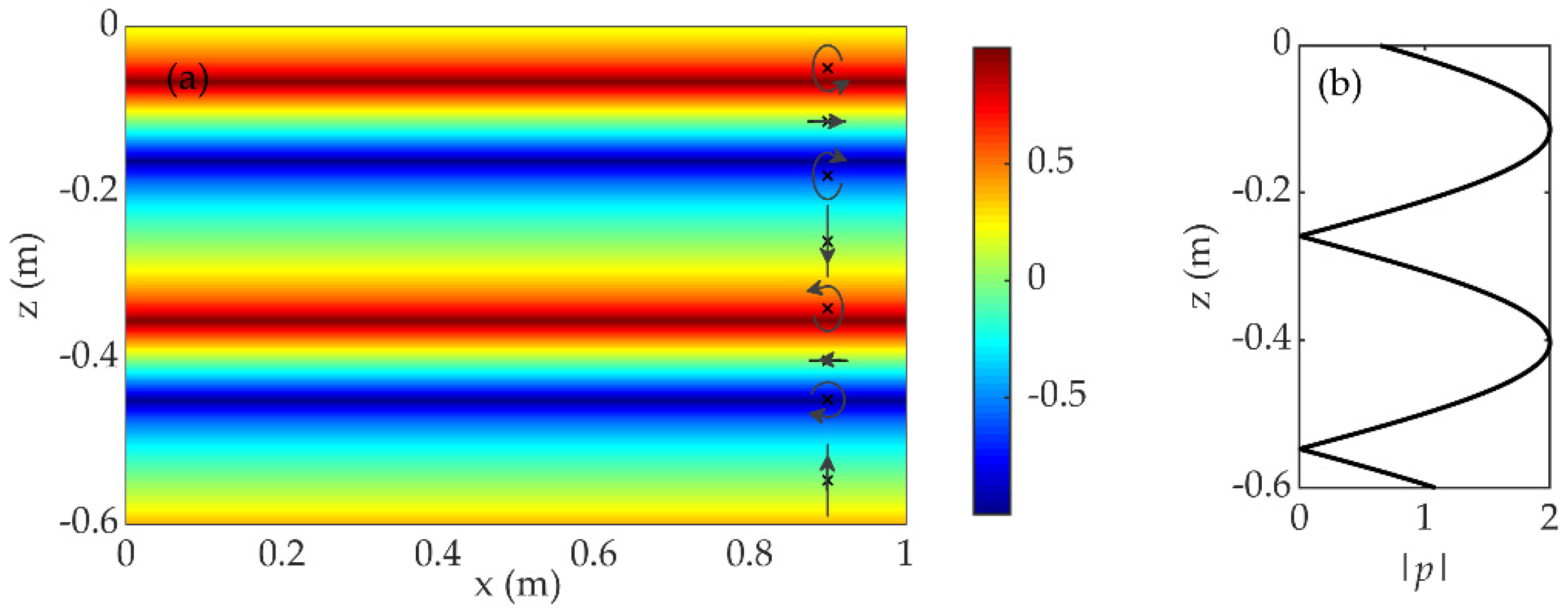
3.1. The Properties of Pressure, Particle Velocity, and Complex Intensity near the Baffle Based on the Euler Description

According to the Euler description, we fix the coordinate system in space and introduce the spatial coordinates x and z and time t as variables to describe the acoustic properties at a given point and time. The properties of the pressure, the particle velocity, and the complex intensity near the baffle are analyzed numerically in this part.

In the free field, the pressure magnitude is the same everywhere, and the points with the same phase of the pressure are on the same plane that is perpendicular to the sound propagation direction. Moreover, the pressure and the complex particle velocity at the same position are in phase. Therefore, the field can be characterized as purely active intensity, which means the reactive intensity is zero according to Equation (30). In particular, the particle velocity direction and the active intensity direction are consistent with the azimuth of the source, which provides a theoretical support for the DOA estimation using a single vector hydrophone in the free space [27,28]. However, the acoustic field near the planar cavity baffle is determined by the incident wave and the reflected wave together. Therefore, the acoustic vector field near the planar cavity baffle is more complex than that in the free space.

According to Equation (27), the spatial structure of the complex pressure magnitude and the complex pressure phase near the planar cavity baffle are provided in Figure 2. As shown in Figure 2, the complex pressure magnitude is the same in the tangential direction due to the infinite assumption of the baffle. The interference fringes appear in the normal direction of the baffle. Moreover, the complex pressure phase is discontinuous at the complex-pressure magnitude zero-planes that are parallel to the reflecting plane.

According to Equations (28) and (29), the complex particle velocity can also be obtained. The spatial structure of the complex particle velocity field of each component is similar to the complex pressure field near the planar cavity baffle, but the spatial positions of strong and weak fringes are obviously different in different components of complex particle velocity. Therefore, the spatial structure of the complex particle velocity field of each component near the baffle is not shown in this paper. In particular, the two real parts of the complex particle velocity indicate the vector of the particle velocity, which is an important property in the acoustic vector field. Moreover, the particle velocity vector field can be better studied by analyzing the singular points of the differential equations of the curve that is tangent to the particle velocity direction. The singular points are those points at which the particle velocity is zero at a certain time.

The equation of the curve that is tangent to the particle velocity direction can be given as

$$\frac{\mathrm{d}z}{\mathrm{d}x}=\frac{\cos \theta \left[\cos J_1\left(x,z\right)-\left|R\right|\cos J_2\left(x,z\right)\right]}{\sin \theta \left[\cos J_1\left(x,z\right)+\left|R\right|\cos J_2\left(x,z\right)\right]},$$

(31)

where

$$J_1\left(x,z\right)=k_{0}x\sin \theta +k_{0}z\cos \theta -\omega t,$$

(32)

$$J_2\left(x,z\right)=k_{0}x\sin \theta -k_{0}z\cos \theta -\omega t+{\phi }_R,$$

(33)

${\phi }_R$ is the phase of complex reflection coefficient, and $\left|R\right|$ is the complex reflection modulus. If the numerator and denominator of the expression on the right side of Equation (31) are expanded by Taylor near the singular point $(x_0,z_0)$ in power series starting with the first powers of x and z, it can be written as

$$\frac{\mathrm{d}z}{\mathrm{d}x}=\frac{\cos \theta \left[\sin \theta \left(x-x_0\right)T_1+\cos \theta \left(z-z_0\right)T_2\right]}{\sin \theta \left[\sin \theta \left(x-x_0\right)T_2+\cos \theta \left(z-z_0\right)T_1\right]},$$

(34)

where

$$T_1=-k_0\sin J_1\left(x_0,z_0\right)+\left|R\right|k_0\sin J_2\left(x_0,z_0\right),$$

(35)

$$T_2=-k_0\sin J_1\left(x_0,z_0\right)-\left|R\right|k_0\sin J_2\left(x_0,z_0\right).$$

(36)

From Equations (28) and (29), it is easy to derive that the singular points satisfy the following equation

$$\{\begin{array}{c}\cos J_1\left(x_0,z_0\right)=0\\ \cos J_2\left(x_0,z_0\right)=0\end{array}.$$

(37)

Additionally, the reflection coefficient of the underwater planar cavity baffle is about $\left|R\right|=1$ through calculation. By substituting Equation (37) into Equation (34), the curve equation at a certain time can be obtained as

$$\frac{\mathrm{d}z}{\mathrm{d}x}=\frac{{\cos }^2\theta \left(z-z_0\right)}{{\sin }^2\theta \left(x-x_0\right)}$$

(38)

or

$$\frac{\mathrm{d}z}{\mathrm{d}x}=\frac{x-x_0}{z-z_0}$$

(39)

From Equations (38) and (39), the singular point is a saddle point or nodal point according to the type of the singular point [29].

The particle velocity vector diagram near the planar cavity baffle at different times is presented in Figure 3. As shown in Figure 3, at the region that the $\left|p\right|$ reaches a minimum value, the point at which the total particle velocity is zero is a saddle point; this is because the phase of the $\left|v_x\right|$ is discontinuous at this region. At the region that the $\left|p\right|$ reaches a maximum value, the point at which the total particle velocity is zero is similarly a nodal point; this is because the phase of the $\left|v_z\right|$ is discontinuous at this region. The particle velocity points to or derives from one nodal point at the same time in the particle velocity vector field. Moreover, the saddle point and the nodal point will appear alternately in the normal direction and in the tangential direction, thus forming a coordinated vector field. With the passage of time, these points move in the tangential direction with a velocity of $c_0/\sin \theta$. This shows that the particle velocity directions are different at different points near the planar cavity baffle and the particle velocity direction at the same point changes with time. The particle velocity direction is inconsistent with the sound wave’s propagation direction.

The active intensity and reactive intensity of each component in the normal direction are depicted in Figure 4. The amplitude of acoustic intensity is normalized by parameter $1/\left(2{\rho }_0{c}_0\right)$. As can be observed in Figure 4, the z component of active intensity $I_z$ and the x component of reactive intensity $Q_x$ are zero, which means the complex intensity in the tangential direction is purely active, and the complex intensity in the normal direction is purely reactive. Therefore, the active intensity vector cannot directly reflect the DOA of the source. The values of the x component of active intensity $I_x$ are all positive, but the values of the z component of reactive intensity $Q_z$ are positive or negative. The $Q_z$ is zero at the region where the $\left|p\right|$ reaches a maximum value or a minimum value, and it is in the turning region that $Q_z$ changes sign. These results demonstrate that the power propagates parallel to the planar cavity baffle that is the projection direction of incident wave on baffle, and the standing wave is formed in the normal direction. Moreover, the period of $I_x$ and $Q_z$ is $\lambda /2\cos \theta$, which is determined by incident frequency and incident angle in the normal direction. The spatial amplitudes of $I_x$ and $Q_z$ are only related to the incident angle.

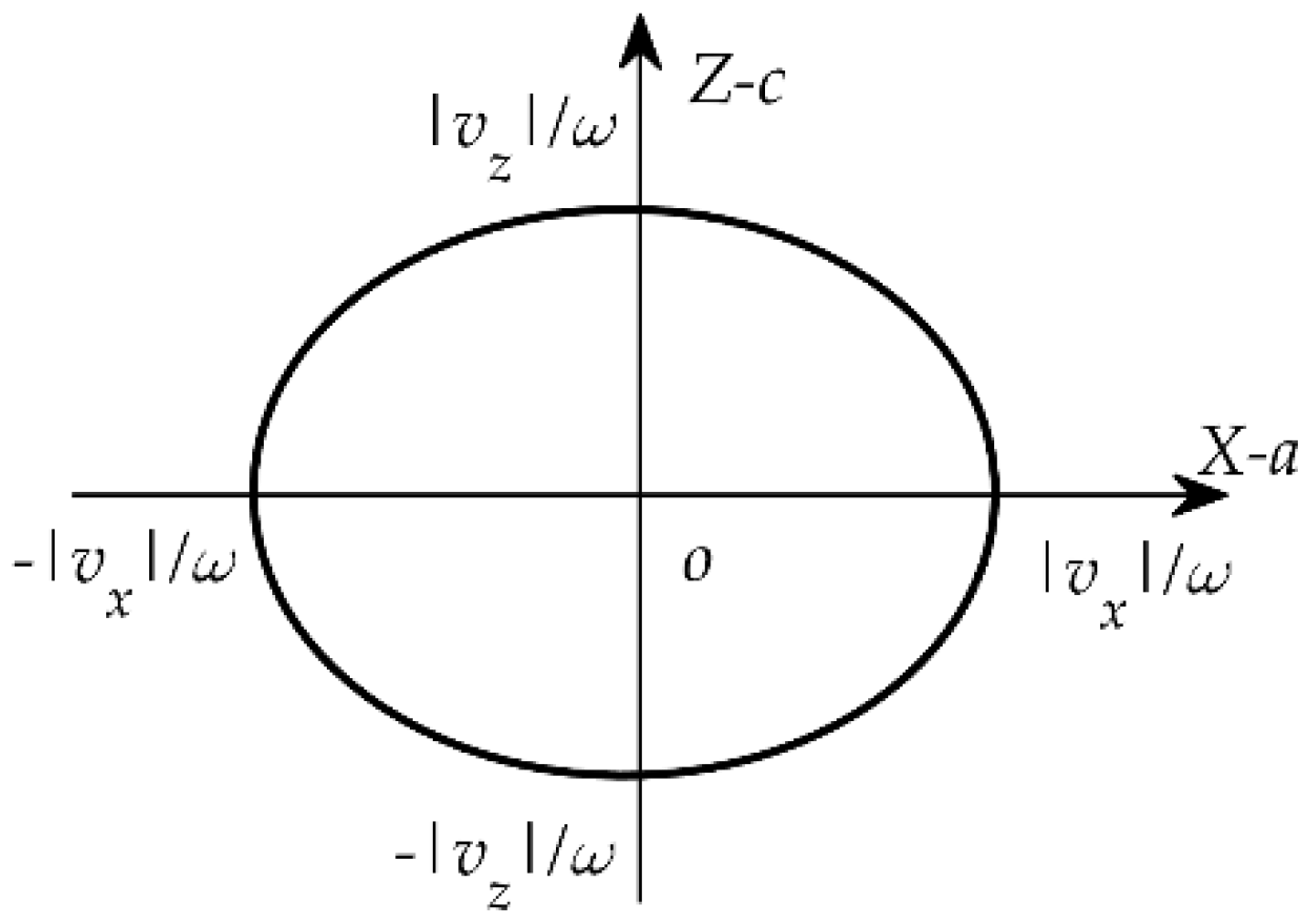
3.2. The Properties of the Acoustic Particle Motion near the Baffle Based on the Lagrange Description

In the Lagrange description, each physical quantity can be expressed as a function of the initial position of the particle and time. Within the approximate range of linear acoustics, the difference between Euler description and Lagrange description can be ignored. The results of the two methods are approximately equal [30]. Integrating the complex particle velocity expressions of Equations (28) and (29) over time and taking the real part can yield particle displacements. Assuming that the initial position of the particle is $(a,c)$ in the xoz plane, the particle position at an arbitrary moment is

$$X(a,c,t)=a+\mathrm{Re}\left(\int v_x(a,c,t)dt\right),$$

(40)

$$Z(a,c,t)=c+\mathrm{Re}\left(\int v_z(a,c,t)dt\right).$$

(41)

For convenience, substituting $v_{x,z}(a,c,t)=\left|v_{x,z}\right|{\mathrm{e}}^{\mathrm{i}\left({\phi }_{x,z}-\omega t\right)}$ into Equations (40) and (41), we have

$$X(a,c,t)-a=A_s\cdot \sin \left(\omega t-{\phi }_x\right),$$

(42)

$$Z(a,c,t)-c=C_s\cdot \sin \left(\omega t-{\phi }_z\right),$$

(43)

where $A_s=\left|v_x\right|/\omega$, $C_s=\left|v_z\right|/\omega$.

The acoustic particle motion trajectory near the planar cavity baffle satisfies the equation

$$\frac{{(X-a)}^2}{A_s^2{\sin }^2{\phi }_{xz}}+\frac{{(Z-c)}^2}{C_s^2{\sin }^2{\phi }_{xz}}-\frac{2(X-a)(Z-c)\cos {\phi }_{xz}}{A_s{C}_s{\sin }^2{\phi }_{xz}}=1,$$

(44)

where ${\phi }_{xz}$ is the phase difference of two components of the particle velocity. In the free field, the particle velocity of x direction and z direction are in phase, the acoustic particle motion is a straight line, and the direction of the straight line reflects the azimuth of the source. However, the two components of particle velocity are out of phase in the acoustic field due to the acoustic baffle. It can be seen that the ellipse is the most common physical pattern of the acoustic particle motion near the underwater planar cavity baffle according to the equation. The difference of the complex particle velocity between the two components determines the particle motion.

The complex particle displacement of tangential and normal direction will have unequal amplitudes and phases, tracing an ellipse of a certain size, shape, and orientation. Now we will study the shape and orientation of the particle motion near the baffle. According to Ref. [21], the orientation angle is

$$\alpha =\mathrm{Re}\left[{\tan }^{-1}\left(u_z/u_x\right)\right],$$

(45)

And the ellipse aspect ratio is

$$b/a=\tanh \left[\mathrm{Im}\left\{{\tan }^{-1}\left(u_z/u_x\right)\right\}\right],$$

(46)

where $u_z$ and $u_x$ is the complex particle displacement of normal and tangential direction, respectively. The orientation angle is defined as the rotation angle between the major axis of the elliptical particle motion and the x-axis. The ellipse aspect ratio is between −1 and 1, its sign can describe the particle motion direction, and its absolute value is the ratio of the real-valued semiminor axis to the real-valued semimajor axis of the ellipse, which can describe the similarity between the particle motion trajectory and the circle. In the frequency domain, these parameters can also be obtained using ratios of complex velocity or acceleration, as the harmonic factors cancel.

The spatial distribution of the ellipse aspect ratio near the planar cavity baffle is shown in Figure 5a, and the spatial distribution of $\left|p\right|$ in the normal direction is shown in Figure 5b. The arrows in Figure 5a show the acoustic particle motion trajectory (highly exaggerated) followed over 3/4 of a cycle. Note how the direction in which the particle moves changes. In Figure 5, it can be seen that the ellipse aspect ratio is the same in the tangential direction, and it changes periodically between −1 and $1$ in the normal direction, which means the shapes of particle motion are continuously changing in the normal direction. As shown in Figure 5a,b, the particle motion (and thus particle velocity) falls on a straight line whose direction is the tangential direction at the region where the $\left|p\right|$ reaches a maximum value, and it is also the turning region of counterclockwise motion to clockwise motion. Moreover, the particle motion (and thus particle velocity) falls on a straight line whose direction is the normal direction at the region that the $\left|p\right|$ reaches a minimum value, and it is also the turning region of clockwise motion to counterclockwise motion. Since the amplitude of the complex particle velocity and the phase difference between the two components are the same in the tangential direction, the particle motion is the same in this direction according to Equation (44), which is consistent with the results obtained in Figure 5. Therefore, Figure 6 only depicts the phase difference between the complex particle velocity of the x direction and the z direction, the ellipse aspect ratio, and the orientation angle near the baffle in the normal direction. It can be seen that the phase difference between the two components of particle velocity is $90{}^{\circ }$, which is due to the fact that the reflection coefficient of the baffle is about $\left|R\right|$ = 1. This causes the orientation angle to be $0{}^{\circ }$ or $90{}^{\circ }$, which means the major axis of particle motion is the x-axis or the z-axis. Furthermore, the ellipse aspect ratio is positive and the particle moves counterclockwise if ${\phi }_{zx}=90{}^{\circ }$, and the ellipse aspect ratio is negative and the particle moves clockwise if ${\phi }_{zx}=-90{}^{\circ }$.

According to Figure 6 and Equation (44), the pattern of acoustic particle motion near the underwater planar cavity baffle is demonstrated in Figure 7. As shown in Figure 7, the real-valued semimajor axis and the real-valued semiminor axis of the ellipse are $\left|v_x\right|/\omega$ and $\left|v_z\right|/\omega$, and the major axis of particle motion is x-axis or z-axis. The direction of particle motion is continuously changing with time, which can be seen in Figure 3. Therefore, the direction of particle velocity cannot reflect the azimuth of the source, and the orientation of the major axis of the elliptical particle motion can also not reflect the azimuth of the source.

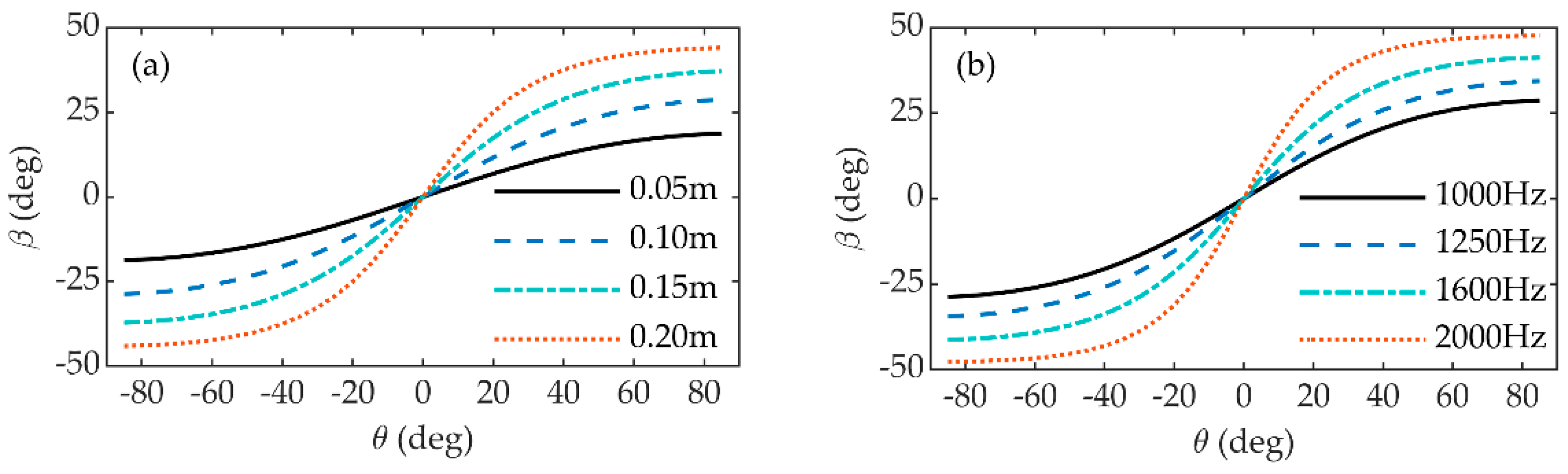
4. The Application of the Properties of the Acoustic Vector Field near the Baffle

The properties of the acoustic vector field near the baffle are derived in Section 3. This section presents a method to estimate the DOA in the presence of the baffle based on these properties.

The particle motion contains the information of the incident acoustic field. We define a parameter $\beta \left(\theta \right)$ according to the orientation angle and the ellipse aspect ratio, that is,

$$\beta \left(\theta \right)=-{\tan }^{-1}\left\{\mathrm{Im}\left\{\tan \left\{1/\left[\alpha +i{\tanh }^{-1}\left(b/a\right)\right]\right\}\right\}\right\}.$$

(47)

The parameter $\beta \left(\theta \right)$ can fully represent the particle motion in the determined incident acoustic field. According to Equations (45)–(47), the parameter $\beta$ can be obtained by using the ratios of complex particle velocity or complex intensity in the frequency domain as follows:

$$\beta \left(\theta \right)=-\mathrm{Im}\left(V_x/V_z\right)=\mathrm{Im}\left(P{V}_x^{*}/P{V}_z^{*}\right).$$

(48)

where $P$ is the Fourier transform of $p$ in the time, and $V_x$ and $V_z$ are the Fourier transform of $v_x$ and $v_z$ in the time. Moreover, because the combined processing of pressure and particle velocity can obtain a higher output signal-to-noise ratio [27,28], it is the best to use the complex intensity ratio in two directions to calculate parameter $\beta$ from the acoustic data. The DOA estimation value $\widehat{\theta }$ can be obtained by substituting the estimated parameter $\widehat{\beta }$ into the inverse function of $\beta \left(\theta \right)$. The parameter $\beta$ obtained in the following simulation is obtained from the complex intensity.

The parameter $\beta \left(\theta \right)$ is shown as a function of the incident angle in Figure 8. From Figure 8a,b, it can be seen that the function $\beta \left(\theta \right)$ depends on the distance between the acoustic vector hydrophone and the baffle d and the incident frequency f. The DOA can be estimated by the parameter $\beta$ if $kd<1.04$. Moreover, as the acoustic vector hydrophone moving far away from the baffle or the frequency increasing, the dynamic range of parameter $\beta \left(\theta \right)$ increases and it becomes easy to estimate the DOA near the normal of the baffle, but the DOA near the tangential direction becomes hard to estimate.

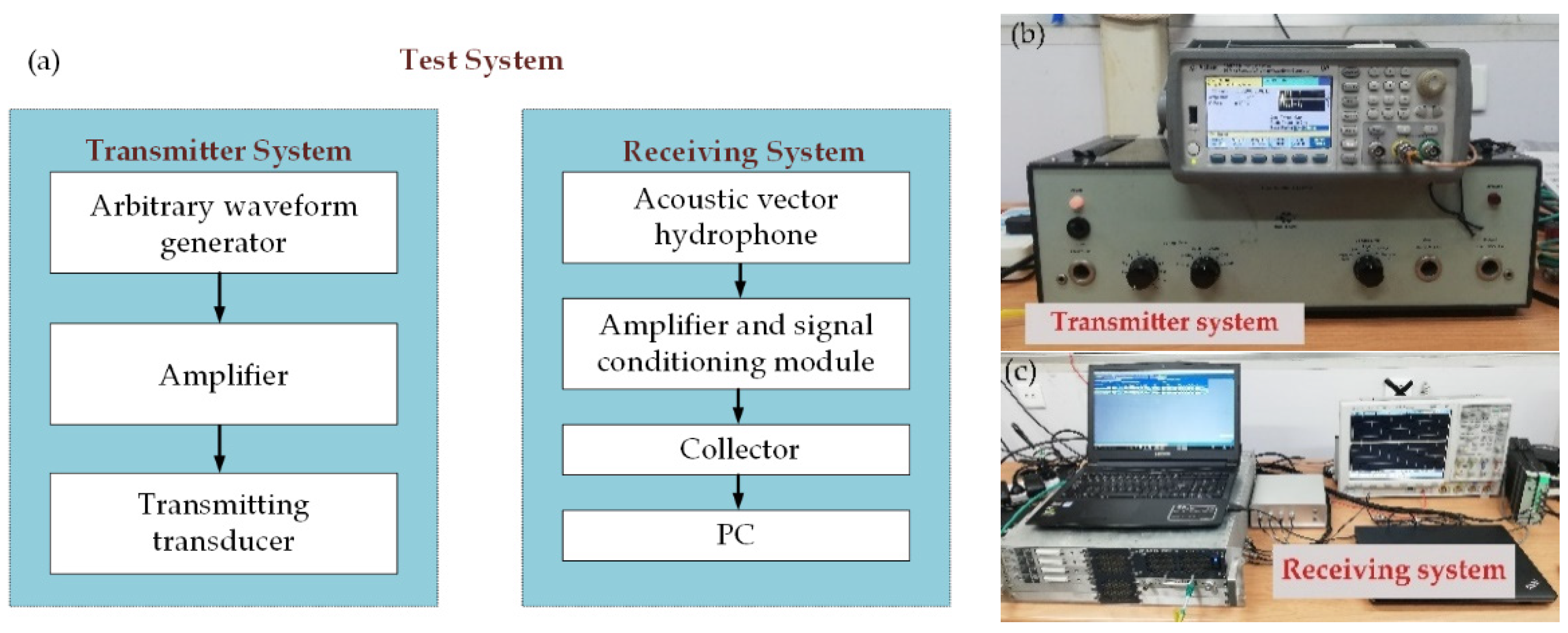
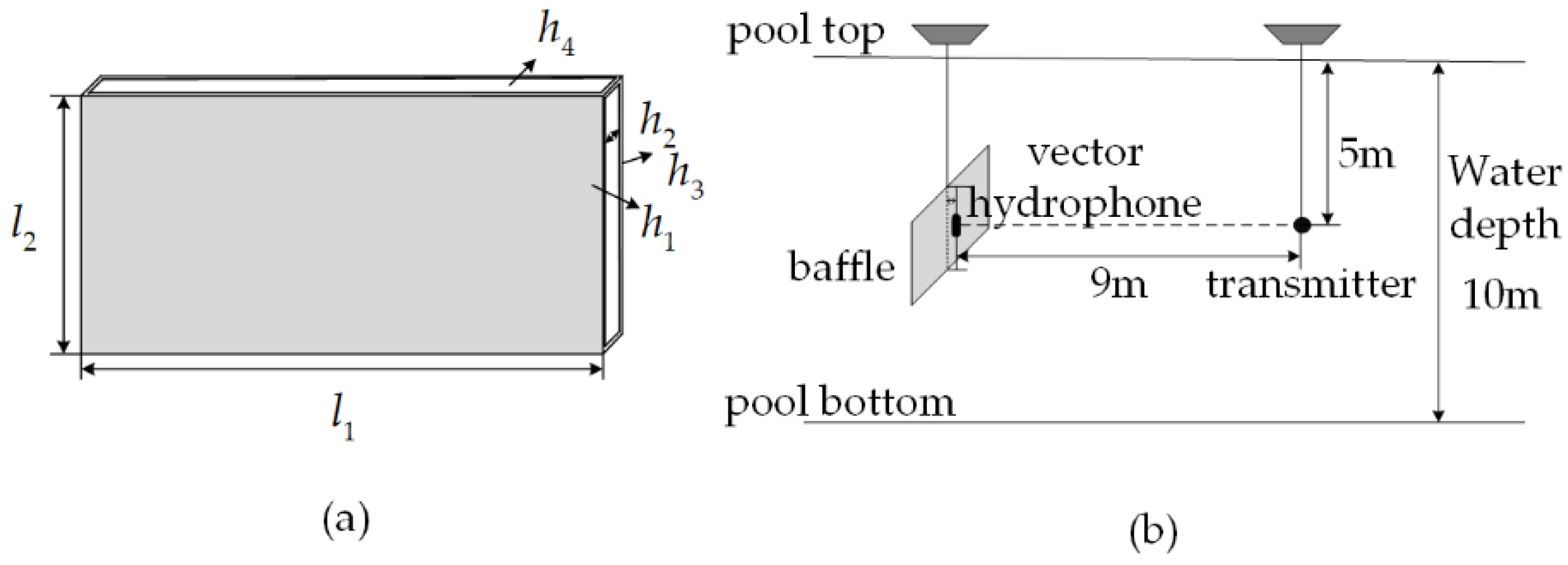
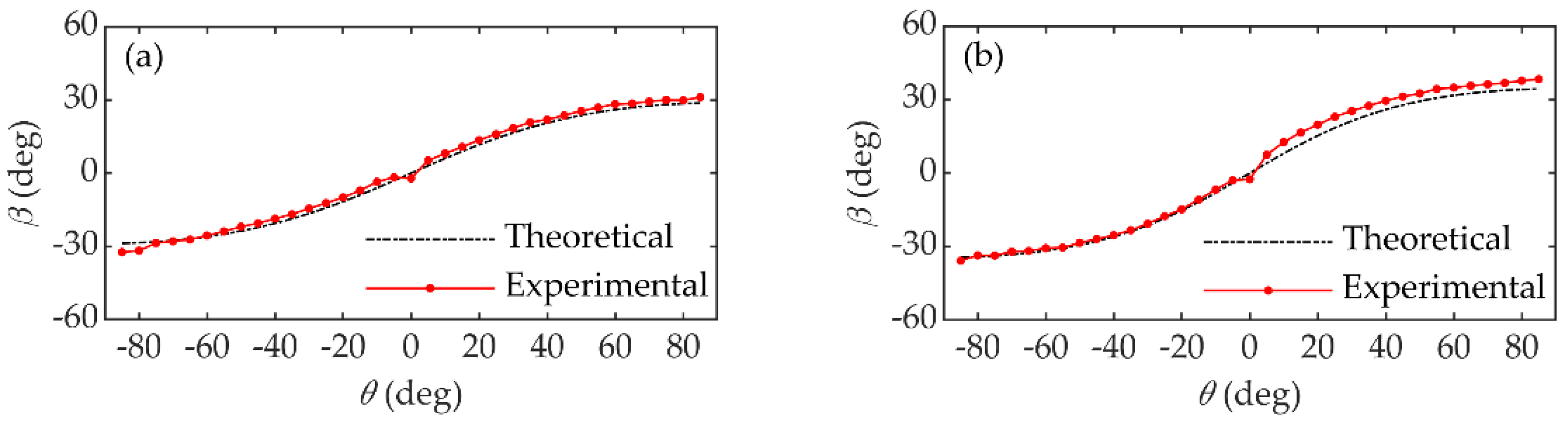
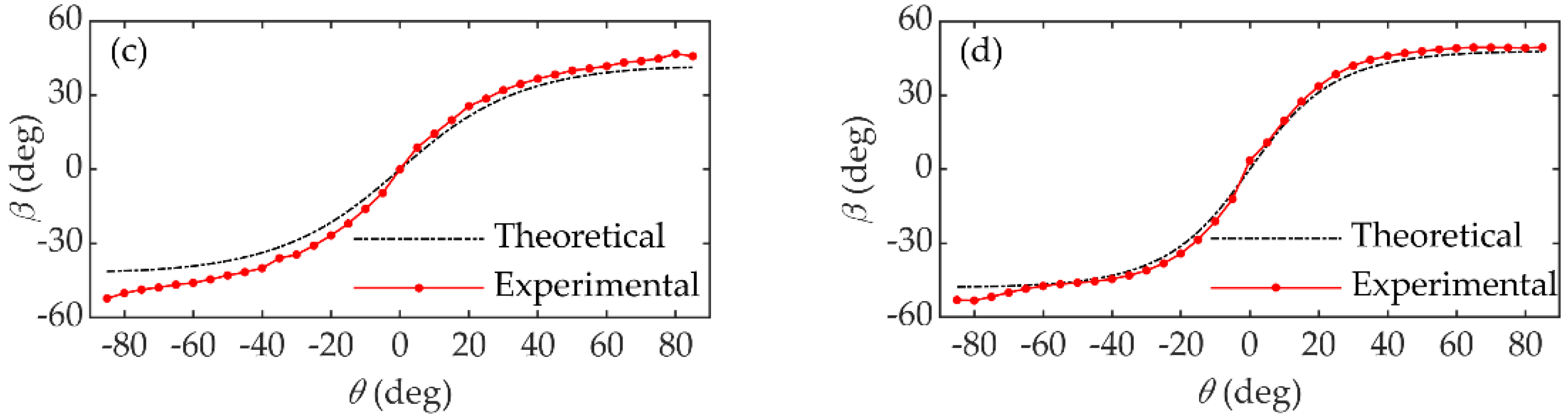
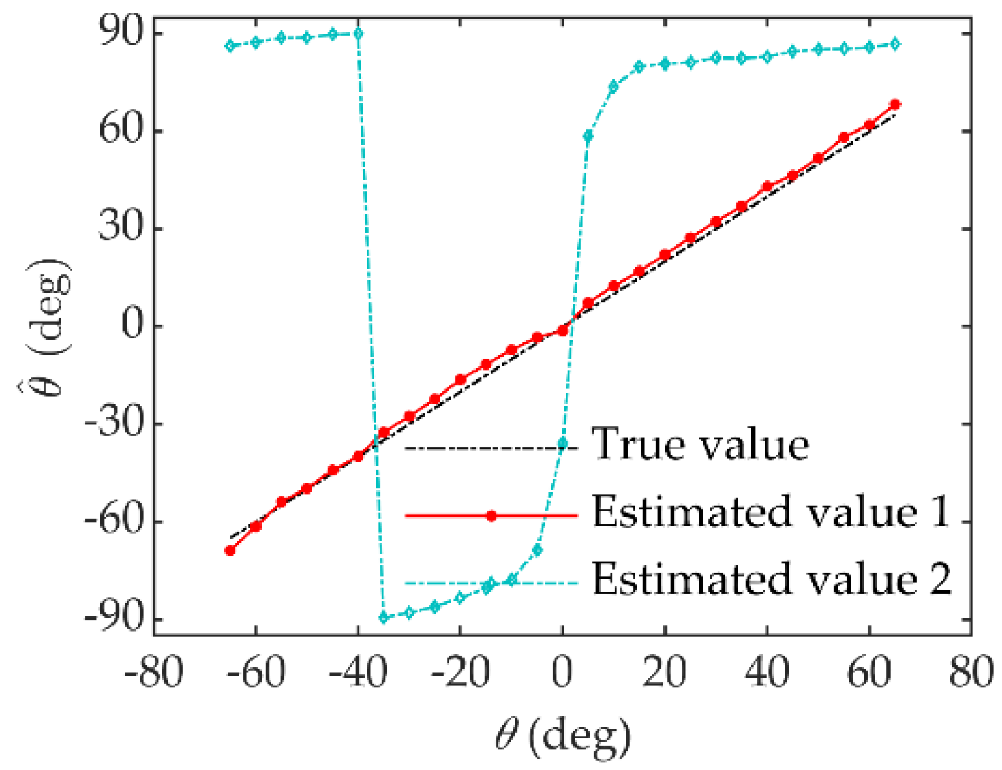
5. Experiment Results

The experiment on the application of the single acoustic vector hydrophone near the underwater planar cavity baffle was carried out in the anechoic tank of the Acoustic Science and Technology Laboratory, Harbin Engineering University. The test system is shown in Figure 9. We can see that the test system includes a transmitter system and a receiving system. The transmitter system consists of an arbitrary waveform generator, amplifier, and transmitting transducer. The receiving system consists of acoustic vector hydrophone, amplifier and signal conditioning module, collector, and laptop. The planar cavity baffle was made in order to verify the theoretical calculations results. The planar cavity baffle is made of steel that forms a closed air cavity, as shown in Figure 10a. The size of the baffle is $l_1\times l_2\times \left(h_1+h_2+h_3\right)=1.6\mathrm{m}\times 0.8\mathrm{m}\times 0.044\mathrm{m}$. The thickness of the front cover plate $h_1$, the back cover plate $h_3$, and the air layer $h_2$ correspond to the values used in the theoretical calculations. The size wall thickness is $h_4=0.008\mathrm{m}$. In the experiment, the hydrophone was about 9 m far from the transmitter. The acoustic vector hydrophone and the transmitter were placed at the depth of 5 m. The depth of the tank was 10 m. Figure 10b shows the schematic diagram of deployment. Moreover, the change in the incident angle of the source was realized by rotating the baffle. The complex signal was obtained by Hilbert transformation of the recorded signal. The environment of the experiment was quiet.

Figure 11 compares the experimental results and the theoretical results of the function $\beta \left(\theta \right)$ at different frequencies. The experimental results of the parameter $\beta$ are obtained from the complex intensity in the frequency domain. The phase difference between the complex particle velocity is corrected according to the theoretical results. As shown in Figure 11, the function $\beta \left(\theta \right)$ obtained from the experimental data is consistent with that obtained from the theoretical calculation, which verifies the theoretical calculation results. The differences between the experimental results and calculation results may come from the effect of the finite structure of the baffle, the scattering of the flange for connecting the baffle and the rotating device, and the rotation error in the incident angle changed by the rotating device. In addition, the directivity of the particle velocity channel of the hydrophone is not strictly symmetrical at $f=1250\mathrm{Hz}$ and $f=1600\mathrm{Hz}$, which may lead to the asymmetric errors that are observed in the experimental results in Figure 11b,c.

A comparison of the DOA estimation results between the method using the parameter $\beta$ in this paper and the acoustic intensity method in the free space [27,28] at different incident angles is shown in Figure 12. In addition, the estimation error using the method in this paper is shown in Figure 13. It can be seen that the estimation error of the method in this paper is within 5 degrees if the incident angle is from −65° to 65°. Moreover, the DOA cannot be estimated using the acoustic intensity method, as shown in Figure 12, this is because the active intensity direction is not the direction of the target near the baffle. These results indicate that the DOA can be estimated using the parameter $\beta$ that this paper achieved using a single acoustic vector hydrophone mounted near the baffle to estimate the DOA.

6. Conclusions

This paper studies the properties of the acoustic vector field near the underwater planar cavity baffle and presents the method of estimating the DOA using these properties. Based on the Euler description, the results show that the interference structure appears in the acoustic field. The points at which the total particle velocity is zero are saddle points and nodal points in the particle velocity vector field. The direction of particle velocity is inconsistent with the azimuth of the source. It can be approximately concluded that the power propagates parallel to the baffle, which is the projection direction of incident wave on the baffle, and the standing wave is formed in the normal direction. Based on the Lagrange description, the results show that the particle motion is generally an ellipse near the planar cavity baffle, which is related to the incident acoustic field and the position of the hydrophone, and the major axis of ellipse is the x-axis or the z-axis. The acoustic particle motion falls on a straight line at the region where the $\left|p\right|$ reaches anextreme value, and this is the turning region of the change in the acoustic particle motion direction. In view of the above properties, this paper defines a parameter $\beta \left(\theta \right)$ that can fully represent the particle motion, and the DOA can be estimated by this parameter if $kd<1.04$. The experiment of the application of the single acoustic vector hydrophone near the underwater planar cavity baffle is carried out, which verifies the theoretical calculations results and the method of estimating the DOA. The research in this paper serves as a basis for the application of the acoustic vector hydrophone in the presence of the planar cavity baffle.

References

1. Santos, P.; Rodríguez, O.C.; Felisberto, P.; Jesus, S.M. Seabed geoacoustic characterization with a vector sensor array. J. Acoust. Soc. Am. 2010, 128, 2652–2663. [Google Scholar] [CrossRef] [Green Version]
2. Han, X.; Yin, J.; Yu, G.; Du, P. Experimental demonstration of single carrier underwater acoustic communication using a vector sensor. Appl Acoust. 2015, 98, 1–5. [Google Scholar] [CrossRef]
3. Song, X.; Jian, Z.; Zhang, G.; Liu, M.; Guo, N.; Zhang, W. New Research on MEMS Acoustic Vector Sensors Used in Pipeline Ground Markers. Sensors 2015, 15, 274–284. [Google Scholar] [CrossRef] [Green Version]
4. Stinco, P.; Tesei, A.; Dreo, R.; Micheli, M. Detection of envelope modulation and direction of arrival estimation of multiple noise sources with an acoustic vector sensor. J. Acoust. Soc. Am. 2021, 149, 1596–1608. [Google Scholar] [CrossRef]
5. Nehorai, A.; Paldi, E. Acoustic vector-sensor array processing. IEEE Trans. Signal Process. 1994, 42, 2481–2491. [Google Scholar] [CrossRef]
6. Wu, Y.; Li, G.; Hu, Z.; Hu, Y. Unambiguous directions of arrival estimation of coherent sources using acoustic vector sensor linear arrays. IET Radar. Sonar. Navig. 2015, 9, 318–323. [Google Scholar] [CrossRef]
7. Chen, H.; Zhao, J. Coherent signal-subspace processing of acoustic vector sensor array for doa estimation of wideband sources. Signal Process. 2005, 85, 837–847. [Google Scholar] [CrossRef]
8. Kosobrodov, R.A.; Nekrasov, V.N. Effect of the diffraction of sound by the carrier of hydroacoustic equipment on the results of measurements. Acoust. Phys. 2001, 47, 323–328. [Google Scholar] [CrossRef]
9. Barton, J.P.; Wolff, N.L.; Zhang, H.; Tarawneh, C. Near-field calculations for a rigid spheroid with an arbitrary incident acoustic field. J. Acoust. Soc. Am. 2003, 113, 1216–1222. [Google Scholar] [CrossRef]
10. Ji, J.; Liang, G.; Wang, Y.; Lin, W. Influences of prolate spheroidal baffle of sound diffraction on spatial directivity of acoustic vector sensor. Sci. Technol. Sci. 2010, 53, 2846–2852. [Google Scholar] [CrossRef]
11. Roumeliotis, J.A.; Kotsis, A.D.; Kolezas, G. Acoustic scattering by an impenetrable spheroid. Acoust. Phys. 2007, 53, 436–447. [Google Scholar] [CrossRef]
12. Rapids, B.R.; Lauchle, G.C. Vector intensity field scattered by a rigid prolate spheroid. J. Acoust. Soc. Am. 2006, 120, 38–48. [Google Scholar] [CrossRef]
13. Barton, R.J.; Smith, K.B.; Vincent, H.T. A characterization of the scattered acoustic intensity field in the resonance region for simple spheres. J. Acoust. Soc. Am. 2011, 129, 2772–2784. [Google Scholar] [CrossRef]
14. Mann, J.A.; Tichy, J. Acoustic intensity analysis: Distinguishing energy propagation and wave-front propagation. J. Acoust. Soc. Am. 1991, 90, 20–25. [Google Scholar] [CrossRef]
15. Hawkes, M.; Nehorai, A. Acoustic Vector-Sensor Processing in the Presence of a Reflecting Boundary. IEEE Trans. Signal Process. 2000, 48, 2981–2993. [Google Scholar] [CrossRef]
16. Javad, A.S.; Hengameh, K. A Vector-Hydrophone’s Minimal Composition for Finite Estimation-Variance in Direction-Finding Near/Without a Reflecting Boundary. IEEE Trans. Signal Process. 2007, 55, 2785–2794. [Google Scholar] [CrossRef]
17. Dall’Osto, D.R.; Choi, J.W.; Dahl, P.H. Measurement of acoustic particle motion in shallow water and its application to geoacoustic inversion. J. Acoust. Soc. Am. 2016, 139, 311–319. [Google Scholar] [CrossRef]
18. Campbell, J.; Sabet, S.S.; Slabbekoorn, H. Particle motion and sound pressure in fish tanks: A behavioural exploration of acoustic sensitivity in the zebrafish. Behav. Process. 2019, 164, 38–47. [Google Scholar] [CrossRef]
19. Dall’Osto, D.R.; Dahl, P.H. Elliptical acoustic particle motion in underwater waveguides. J. Acoust. Soc. Am. 2013, 134, 109–118. [Google Scholar] [CrossRef]
20. Bonnel, J.; Flamant, J.; Dall’Osto, D.R.; Bihan, N.L.; Dahl, P.H. Polarization of ocean acoustic normal modes. J. Acoust. Soc. Am. 2021, 150, 1897–1911. [Google Scholar] [CrossRef]
21. Osler, J.C.; Chapman, D.M.; Hines, P.C.; Dooley, G.P.; Lyons, A.P. Measurement and Modeling of Seabed Particle Motion Using Buried Vector Sensors. IEEE J. Ocean. Eng. 2010, 35, 516–536. [Google Scholar] [CrossRef]
22. Ebenezer, D.D.; Abraham, P. Effect of multilayer baffles and domes on hydrophone response. J. Acoust. Soc. Am. 1996, 99, 1883–1893. [Google Scholar] [CrossRef]
23. Chen, W.; Hu, S.; Wang, Y.; Yin, J.; Korochensev, V.I.; Zhang, Y. Study on acoustic reflection characteristics of layered sea ice based on boundary condition method. Waves Random Complex Media 2020, 31, 2177–2196. [Google Scholar] [CrossRef]
24. Ye, C.; Liu, X.; Xin, F.; Lu, T. Influence of hole shape on sound absorption of underwater anechoic layers. J. Sound Vib. 2018, 426, 54–74. [Google Scholar] [CrossRef]
25. Gao, N.; Lu, K. An underwater metamaterial for broadband acoustic absorption at low frequency. Appl. Acoust. 2020, 169, 107500. [Google Scholar] [CrossRef]
26. Dall’Osto, D.R.; Dahl, P.H.; Choi, J.W. Properties of the acoustic intensity vector field in a shallow water waveguide. J. Acoust. Soc. Am. 2012, 131, 2023–2035. [Google Scholar] [CrossRef]
27. Gordienko, V.A.; Krasnopistsev, N.V.; Nasedkin, A.V.; Nekrasov, V.N. Estimation of the Detection Range of a Hydroacoustic System Based on the Acoustic Power Flux Receiver. Acoust. Phys. 2007, 53, 721–729. [Google Scholar] [CrossRef]
28. Felisberto, P.; Rodriguez, O.; Santos, P.; Ey, E.; Jesus, S. Experimental results of underwater cooperative source localization using a single acoustic vector sensor. Sensors 2013, 13, 8856–8878. [Google Scholar] [CrossRef] [Green Version]
29. Karman, T.V.; Biot, M.A. Mathematical Methods in Engineering, 1st ed.; McGraw-Hill Book Company: New York, NY, USA; London, UK, 1940; pp. 150–158. [Google Scholar]
30. Morse, P.M.; Ingard, K.U. Theoretical Acoustics, 2nd ed.; McGraw-Hill Book Company: New York, NY, USA, 1968; pp. 234–239. [Google Scholar]
Figure 1. The schematic diagram of harmonic plane waves exciting on the planar cavity baffle.
Jmse 10 00138 g001
Figure 2. (a) The spatial structure of the complex-pressure magnitude near the planar cavity baffle; (b) the spatial structure of the complex pressure phase near the planar cavity baffle. In (a,b), the time is t = 1 / 3   ms .
Jmse 10 00138 g002
Figure 3. The particle velocity vector diagram near the planar cavity baffle, where the red circle represents the nodal point and the blue cross represents the saddle point. (a) t = 1 / 12   ms ; (b) t = 1 / 6   ms ; (c) t = 1 / 4   ms ; (d) t = 1 / 3   ms .
Jmse 10 00138 g003aJmse 10 00138 g003b
Figure 4. The active intensity and reactive intensity of each component in the normal direction.
Jmse 10 00138 g004
Figure 5. (a) The spatial distribution of the ellipse aspect ratio near the planar cavity baffle. The arrows show the acoustic particle motion trajectory (highly exaggerated) followed over 3/4 of a cycle. (b) The spatial distribution of | p | in the normal direction.
Jmse 10 00138 g005
Figure 6. (a) The phase difference between the complex particle velocity in the x direction and z direction near the baffle in the normal direction. (b) The ellipse aspect ratio of the particle motion near the baffle in the normal direction. (c) The orientation angle of the particle motion near the baffle in the normal direction.
Jmse 10 00138 g006
Figure 7. The pattern of acoustic particle motion trajectory near the underwater planar cavity baffle.
Jmse 10 00138 g007
Figure 8. (a) The parameter β ( θ ) shown as a function of incident angle under different acoustic vector hydrophones positions, where the incident frequency is f = 1000   Hz . (b) The parameter β ( θ ) shown as a function of incident angle under different incident frequencies, where the distance between the baffle and the hydrophone is d = 0.10   m .
Jmse 10 00138 g008
Figure 9. (a) The schematic diagram of the test system. (b) The photo of the transmitter system. (c) The photo of the receiving system.
Jmse 10 00138 g009
Figure 10. (a) The planar cavity baffle used in the experiment. (b) The schematic diagram of deployment.
Jmse 10 00138 g010
Figure 11. The comparison of the experimental results and the theoretical results of the function β ( θ ) at different frequencies, where the distance between the baffle and the hydrophone is d = 0.10   m . (a) f = 1000 Hz; (b) f = 1250 Hz; (c) f = 1600 Hz; (d) f = 2000 Hz.
Jmse 10 00138 g011aJmse 10 00138 g011b
Figure 12. The DOA estimation results at different incident angles, where the estimated value 1 is obtained from the parameter β in this paper, and the estimated value 2 is obtained from the acoustic intensity method in the free space.
Jmse 10 00138 g012
Figure 13. The estimation error using the parameter β at different incident angles.
Jmse 10 00138 g013
Publisher’s Note: MDPI stays neutral with regard to jurisdictional claims in published maps and institutional affiliations.