Improving Operational Ocean Models for the Spanish Port Authorities: Assessment of the SAMOA Coastal Forecasting Service Upgrades

Abstract

The Puertos del Estado SAMOA coastal and port ocean forecast service delivers operational ocean forecasts to the Spanish Port Authorities since 01/2017 (originally set-up for 9 ports). In its second development phase (2019–2021), the SAMOA service has been extended to 31 ports (practically, the whole Spanish Port System). Besides, the next generation of the SAMOA service is being developed. Research is being focused on (1) updating atmospheric forcing (by combining the AEMET HARMONIE 2.5 Km forecasts and the IFS-ECMWF ones), (2) upgrading the circulation model (ROMS), and (3) testing new methodologies to nest SAMOA systems in the Copernicus IBI-MFC regional solution (with emphasis on its 3D hourly dataset). Evaluation of specific model upgrades is here presented. Model sensitivity tests have been assessed using the available in-situ and remoted sensed (i.e., RadarHF) observations. The results show that SAMOA outperforms IBI-MFC in sea level forecasting at meso- and macro-tidal environments. Improvements by the herein proposed upgrades are incremental: some of these set-ups were used in the last SAMOA operational releases (i.e., the SAM_INI and the SAM_ADV ones; the later currently in operations), whereas the latest test (SAM_H3D) ensures more nesting consistency with the IBI-MFC and improves significantly surface currents and sea-surface temperature simulations.

1. Introduction

Operational oceanography, as defined by EuroGOOS (European Global Ocean Observing System [1]) is the activity of systematic and long-term routine measurements of the ocean and atmosphere, and their fast interpretation and dissemination. Operational Oceanography is rapidly maturing, and its capabilities are being enhanced, mostly in response to a growing demand of regularly-updated ocean information. End-users and stakeholders are key to sustain operational oceanographic systems, as well as to foster new ones.

A complete list of the range of services and a description of how end-users and stakeholders use these operational services goes beyond the scope of this introduction (see Schiller et al., 2018 and Davidson et al., 2019 for more extensive reviews [2,3]). However, in general, primary sectors supported by operational oceanographic services are those related to improve the safety and efficiency of marine activities. Many of the existing operational oceanographic services focuses on regional coastal waters, where most of the protection of marine environments in sensitive habitats and human activities occurs (De Mey-Frémaux et al., 2019 [4]).

Among coastal activities, the ones related to port activity are certainly important due to the role that ports play in global and national economies. Note that the total gross weight of goods handled in EU (European Union) ports was estimated above 3.8 billion tonnes in 2015. The Spanish Port System contributes to this activity, handling 447 million tonnes during 2015, with a 4.5% of annual growth in the 2010–2015 period (EU EuroStat 2017 [5]). Approximately, 85% of total Spanish imports and 60% of exports are channelled through ports.

However, the ports are highly impacted by extreme met-ocean drivers (especially wind, waves, surface currents and sea level). Physical environment constrains Port equipment and their activities during all phases of Port life (from its design phase, in the planning tasks and during daily operations). Thus, oceanographic historical or reanalysis data are needed to be used in design criteria for offshore structures. Coastal infrastructure and maritime industries also require short-term high-resolution forecasts of wind, wave and current to manage their operational decisions. At a wider temporal horizon, longer-term forecasts and climate projections are needed for strategic decisions, port adaptation and planning. In order to answer to these complex challenges, the Spanish Port System launched SAMOA (Sistema de Apoyo Meteorológico y Oceanográfico a las Autoridades portuarias—System of Meteorological and Oceanographic Support for Port Authorities; Álvarez Fanjul et al., 2018 [6]). From 2014, Puertos del Estado (PdE) has led this SAMOA initiative developing and providing high-resolution met-ocean operational products to feed Decision Support Systems of the Spanish Port Authorities.

This SAMOA initiative combines met-ocean observation, ocean modelling and end-user service tools. One of the SAMOA components (the one referred in this work) is focused on the design and implementation of very high-resolution ocean circulation forecast systems, able to solve from coastal to very local scales within the ports. Sotillo et al., (2019) [7] provides an extensive description of this SAMOA integrated coastal/port forecast service. This system solves governing equations for ocean currents, sea level, temperature, salinity and concentrations of tracers; as one of the building blocks of any operational oceanographic systems aimed to forecast physical coastal processes.

In that sense, in the last decade, a great variety of operational ocean models were used, mostly at global (Lellouche et al., (2013, 2018), Liu et al., 2021 [8,9,10]) and basin scales on European Seas, based on different model codes (with different physical parameterization sets), spanning a wide range of spatial and temporal scales, using different forcing data sets and relying on data assimilation methods (Bell et al., 2009; Bell et al., 2015; Tonani et al., 2015 [11,12,13]). Today, the Copernicus Marine Service (CMEMS; https://marine.copernicus.eu/ accessed on 18 January 2022 [14]), focused on global and regional scales in European basins, is well-established and the sustained availability of its “core” operational ocean products has favoured the proliferation of “downstream” services devoted to coastal monitoring and forecasting (Letraon et al.; 2019 [15]). Capet et al., (2019) [16] in their review of current European capacity in terms of operational marine and coastal modelling systems, map 49 organizations around Europe delivering 104 operational model systems simulating mostly hydrodynamics, biogeochemistry and sea waves at regional and coastal scales. The PdE SAMOA coastal forecast model applications for Spanish ports, are nested into the CMEMS forecast solution for the Iberian-Biscay-Ireland (IBI) regional seas (Sotillo et al., 2015, Aznar et al., 2016 [17,18]), thus contributing to this European coastal model capacity.

In their detailed review on the basis of coastal modelling, Kourafalou et al., (2015) [19] pointed out that advancement of coastal ocean forecasting systems requires continuous scientific progress in several key topical areas. Among them, the following research lines were identified as priority ones to evolve the SAMOA service: (i) to understand primary mechanisms driving coastal circulation; (ii) to develop adequate methods to dynamically embed coastal systems in larger scale systems; and (iii) to include in downscaled solutions methods to adequately represent air–sea and land interactions, involving atmosphere-wave-ocean coupling. Dealing with these primary science topics was fundamental to face the initial SAMOA development phase (2014–2017) that resulted in nine new SAMOA coastal model applications (running operationally since 2017), as well as to align the research needed to improve the SAMOA circulation models. This second development phase, the SAMOA-2 Project (2019–2021), allowed to extend the SAMOA forecast service to a higher number of Spanish Ports (31) and to upgrade the ocean model applications in which the SAMOA service is based.

This contribution presents the research conducted to develop the next generation of SAMOA coastal circulation model applications. This research has focused on improving the SAMOA forecasts through three main objectives:

(i)

Enhancing the ocean model set-up.

(ii)

Updating the atmospheric forcings and the methodology to introduce their effect on the solution.

(iii)

Testing a new nesting methodology by benefiting from a new Copernicus IBI-MFC regional 3D hourly forecast product.

A complete description of the sensitivity tests performed to improve the coastal model that support the SAMOA operational service, joint with the quality assessments via extensive model validation (using different local available in-situ and remote sense observations), is herein provided.

The paper is organised as follows: Section 2 outlines the PdE SAMOA initiative, describing its objectives, components and major benefits as well as the amelioration axes followed in its currently on-going second development phase (SAMOA-2). Section 3 describes the model sensitivity tests performed aimed to improve the SAMOA model solution. Section 4 presents a detailed discussion of the results with an analysis of the proposed SAMOA updates in the different port domains. Finally, Section 5 summarises main conclusions and gives a look ahead to on-going and future research topics that may enhance SAMOA operational forecast capabilities.

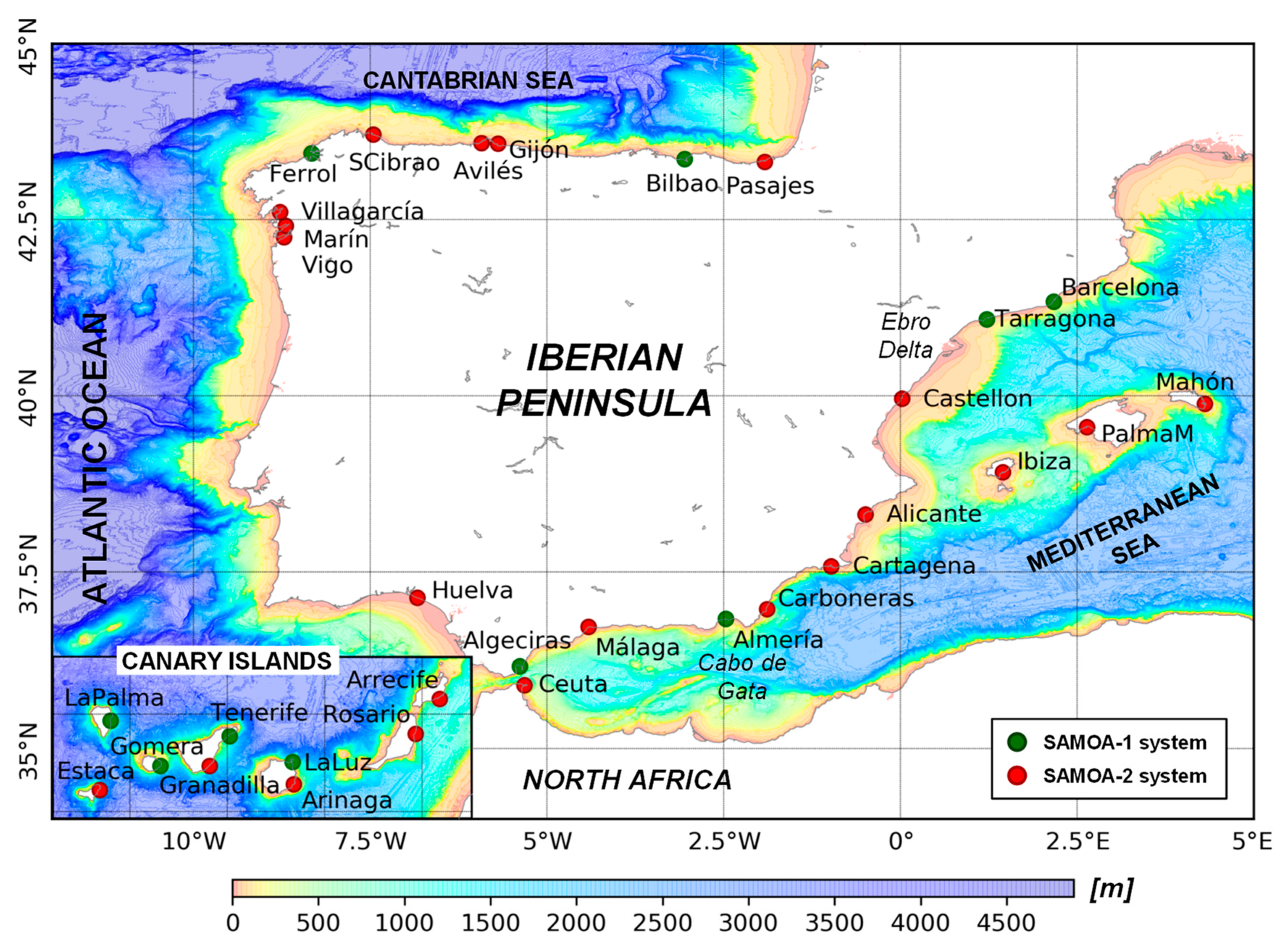
2. The Operational Context: The PdE SAMOA Coastal Forecast Service and Its Second Development Phase (SAMOA-2)

Since the mid-1990s, PdE has acted as an operational oceanographic centre, sustaining an integrated multiplatform ocean monitoring and forecasting system that provides service from regional to coastal scales. Met-ocean parameters, such as wind, waves, sea-level and currents have been extensively monitored and forecasted. Main applications range (i) the safety of port operations, (ii) impacts on ship draught allowance, (iii) water quality and (iv) navigation and piloting activities.

The SAMOA initiative, co-financed by PdE and the Spanish Port Authorities, was born in 2014 as an answer to the complex port needs in terms of coastal and local met-ocean information (Álvarez Fanjul et al., 2018 [6]). SAMOA aims to enhance the PdE traditional operational oceanographic service, implementing new operational systems for each Port Authority, with tailor-made operational met-ocean information, as well as some added value products, previously requested by each Port Authority.

The SAMOA service is organized as a modular infrastructure, with some of the SAMOA modules focused on enhancing near-real-time monitoring (i.e., by means of local upgrading of current PdE observational networks with specific instrumentation), whereas some others are focused on implementing new local high-resolution forecast applications for atmosphere, waves and ocean circulation. The enhancement of PdE model capabilities within SAMOA, and its follow-up in SAMOA-2, has been certainly significant, being a total of 17 new high-resolution atmospheric models (1 km resolution, based on HARMONIE model), 20 wave agitation models (5 m resolution mild slope model applications) and 31 circulation models (70 m ROMS model set-ups) developed and operationally implemented. The SAMOA modular architecture allows each Port Authority to decide what specific SAMOA services are needed to be implemented in their ports, mainly addressing their specific needs for met-ocean information. A total 47 ports from 28 Spanish Port Authorities benefited from these new SAMOA modelling and monitoring capabilities.

To properly exploit new SAMOA added-value products, a specific tool was developed for the Ports: The CMA (Cuadro de Mando Ambiental or Environmental Control Panel). This CMA dashboard is a tailor-made web service that provides easy and customized access to operational met-ocean information in the ports, as well as advanced viewing capabilities (see snapshot in Figure 1a) and other end-user services (such as an alert system (through email/SMS), or a tool to automatically generate daily bulletin reports with environmental conditions at selected locations). Managers in the ports grant access to this CMA tool and they can define different levels of user permissions. A growing community of 1913 port registered users benefits from the CMA tool.

With respect to ocean circulation forecast, and after running regional ocean circulation model applications for more than a decade (i.e., the Spanish ESEOO system; Sotillo et al., 2008 [20]), PdE does not run anymore a regional forecast component, relying since 2014 for these scales on the Copernicus Marine IBI-MFC regional forecast service (Aznar et al., 2016 [18]). This use of Copernicus regional products (currently delivering forecast products at 1/36° resolution that covers all the Spanish waters) has allowed PdE to focus their ocean modelling resources on running very high-resolution models at specific hot spots (p.eg. the Gibraltar Strait and nearby areas, operationally covered by the PdE SAMPA forecast service; Sanchez Garrido et al., 2013 and Sotillo et al., 2016 [21,22]) and on developing the new SAMOA operational downscaled systems for ports, here described.

The related PdE ocean circulation forecast products, updated on a daily basis, can be downloaded through the PdE catalogue (https://opendap.puertos.es/thredds/catalog.html accessed on 18 January 2022 [23]) and visualized through the mentioned CMA Dashboard and the PdE PORTUS web page https://portus.puertos.es/ accessed on 18 January 2022 [24] (see Figure 1b shows a snapshot of the modelled surface current field forecasted for coastal waters nearby the Bilbao harbour).

In SAMOA-2, it was decided to enhance the coastal/port circulation module by adding an extra oil spill forecast service linked to the implementation of a local high-resolution circulation model. This new option allows to have an on-demand use of the PdE oil spill forecast service (based on MedSlik model, De Dominicis et al., 2013 [25]) and to visualize their model outputs through the CMA dashboard (see snapshot of the output tool in Figure 1c). This added oil spill module played a relevant role on fostering the interest of Port Authorities in high-resolution coastal circulation products for their coastal fringes. This Ports’ interest on currents, and mainly on its advective and dispersive effects, is partially explained by the legal commitment that Port Authorities need for ensuring good water quality within harbours (European Parliament, Directive 2019/883 [26]).

In the first SAMOA development phase, nine high-resolution coastal circulation systems were implemented for different Spanish ports located in the Mediterranean, the Iberian Atlantic and the Canary Islands (see green dots in Figure 2). This first SAMOA implementation of high-resolution circulation systems was performed thanks to the collaboration between PdE and the Maritime Engineering Laboratory of the Polytechnic University of Catalonia (LIM/UPC). The same team has continued along SAMOA-2 with the R&D works needed to face the challenge of (i) improving currently existing SAMOA port circulation systems and (ii) to extend this SAMOA forecast service to other requested ports (i.e., multiplying by three the number of Spanish ports where SAMOA coastal forecasts are implemented by 2021).

This noticeable increase in the number of SAMOA Port systems (red dots in Figure 2 shows location of the Spanish ports where new circulation systems are deployed after the SAMOA second development phase) results in an almost complete coverage of the Spanish coast with high-resolution coastal circulation forecasts.

The operational SAMOA local circulation forecast systems daily produce short term (+3 Days) forecasts of 3-D currents and other oceanographic variables, such as temperature, salinity, together with sea level. Each SAMOA system uses the ROMS model (Shchepetkin and McWilliams (2005); present code source and documentation at the ROMS website [27,28]), and consists of two nested regular grids with spatial resolution of ~350 m and ~70 m for the coastal and harbour domains, respectively. The model is forced with very high-resolution atmospheric forcing (provided by the Spanish Meteorological Office AEMET) and it is nested into the core Copernicus IBI regional solution (IBI_PHY hereafter). Figure 3 shows a schematic view of the SAMOA system; for an end-to-end description of the SAMOA model set-up, see Sotillo et al., 2019 [7].

Product quality assessment is a key issue for any operational forecast service (Ryan et al., 2015 [29]). Nevertheless, one of the main bottlenecks identified in the recent review performed by EuroGOOS for European coastal operational ocean model services (Capet et al., 2019 [16]) is the lack of an adequate delivery in near-real-time (NRT) of operational observations. This lack of operational observations, especially on coastal areas, restricts the systematic exploitation of (i) the data assimilation capacities in operational marine modelling systems and (ii) the provision of NRT assessments of operational ocean model products. Note that only 20% of operational models currently available for European seas provide a dynamic uncertainty together with their forecast products.

In the case of SAMOA, an exhaustive NRT validation of the forecast products operationally generated is performed. This operational validation is based on a routine monitoring of the quality of the SAMOA forecast products on a daily and monthly basis. This SAMOA model forecast validation is using all operational ocean observation available in the port and nearby coastal waters. To this aim, an extension of the NARVAL tool (originally developed for the CMEMS IBI MFC regional model solutions (Lorente et al., 2019 [30])) was implemented to validate the SAMOA circulation model products. The comprehensive multi-parametric ocean model skill assessment is performed by using all available operational observational sources in the coastal domains. The list of observational data sources includes satellite L3 and L4 SST products, together with in-situ observations from moorings and tide-gauges, as well as HF-Radars. Further details about the complete list of observational products and platforms used by NARVAL to validate SAMOA can be seen in Sotillo et al., 2019 [7].

Another SAMOA module, consisting of observational campaigns at harbour waters was offered to Port Authorities. These campaigns include at the same time (and for a three month period) deployment of 1 ADCP current-meter, fixed (and repeated) CTD temperature and salinity stations, as well as additional meteorological stations. It is expected that this SAMOA extensive monitoring campaign will help the Ports to increase the knowledge on their waters and to validate the SAMOA met-ocean forecast applications. In that sense, it is remarkable that all Port Authorities (9) who have requested this SAMOA specific in-situ observational port campaign count with a SAMOA Port Circulation Forecast service. However, to assess the model sensitivity tests shown in the present work, only operational observational data sources were used (from PdE HF Radar, tide gauges and coastal or deep-water mooring stations), since data from the new SAMOA observational campaigns were not available when SAMOA model tests were performed.

3. Methodology: Model Sensitivity Tests for Improving the SAMOA Circulation Forecast Services

After more than 4-years running operationally the first 9 SAMOA port forecast services, joint with the continuous quality assessment of their model products (performed throughout the NARVAL validation tool described in the previous section), the following main concerns about the SAMOA solutions were identified:

(i)

Existence of some systematic biases in passive tracers, such as the temperature and salinity fields.

(ii)

Some inconsistencies between SAMOA coastal modelled circulation patterns, compared with those exhibited by the CMEMS IBI-MFC parent solution.

Specific research was conducted with the aim to minimize these limitations via improving the SAMOA model set-up for the forthcoming releases.

External forcing, and particularly the atmospheric one, remains as one of the major issues restricting the accuracy of operational coastal systems. In this sense, improving external atmospheric forcing has been identified as a major concern for enhancing the reliability of high-resolution forecast services (Capet et al., 2019 [16]). Furthermore, the improvement of atmospheric forcing (and a methodology for a better usage in coastal domains) is highlighted in the SAMOA roadmap (outlined in Sotillo et al., 2019 [7]), as one of its three main research lines.

On the other hand, Kourafalou et al., (2015) [19] point out that coastal ocean forecasting systems requires continuous scientific progress in a primary science topic as it is the downscaling from larger scale models, with a need of ad-hoc nesting procedures. This includes assessment of the boundary conditions from the larger scale parent systems to the coastal nested systems, and refinement of the model set-up (including grids, topographic details, forcing data and schemes used as open boundary condition). A challenge for these appropriate nesting procedures is to ensure consistency in the fluxes between the downscaled coastal model and its coarser parent solution. This consistency will avoid problems such as triggering unrealistic gravity transient currents that may unleash spurious dynamical coastal model features.

Consequently, the following three model sensitivity tests were performed:

(i)

To update SAMOA atmospheric forcing data (experiment termed as SAM_INI, hereafter).

(ii)

To improve the ROMS model set-up, with special attention to the open boundary condition treatment; joint with the computation of surface ocean-atmosphere fluxes through a new bulk formulation (SAM_ADV test experiment). Finally also,

(iii)

To test a new nesting methodology taking advantage of the availability of a Copernicus regional 3D IBI hourly forecast product (SAM_H3D). This product allows enhancement of the temporal frequency (from daily to hourly resolution) of the data imposed at boundaries. Moreover, specific physics upgrade was implemented in this configuration experiment.

Table 1. Summary of the main differences among the sensitivity tests conducted. The columns denote the three SAMOA model configurations (SAM_INI, SAM_ADV and SAM_H3D) and the rows the different upgrades. ✔ means included in each model set-up, and ✖ not included.

Feature	SAM_INI	SAM_ADV	SAM_H3D
SAMOA-1 model set-up (as in Sotillo et al. [7])	✔	✔	✔
Use of 2.5 km HARMONIE Atmospheric Forcing	✔	✔	✔
Use of the COARE bulk formulae to compute surface fluxes	✖	✔	✔
Changes in the treatment of Open Boundary Conditions	✖	✔	✔
Use of the new hourly-3D CMEMS IBI-MFC product	✖	✖	✔
Use of new advection scheme for passive tracers and improved surface fluxes physics	✖	✖	✔
Entry into Service (Operational Release)	October 2018	October 2019	To be in 2022

summarises the main differences among the three different model sensitivity datasets. As denoted in Figure 3b, SAM_INI corresponds to the former operational version of SAMOA (active since October 2018 to October 2019), whereas SAM_ADV is the operational set-up currently in production. SAM_H3D will be the forthcoming SAMOA set-up version (to be operationally released in 2022).

All the SAMOA model set-up novelties have been extensively tested. The proposed sensitivity model runs were validated using in-situ and remote sensing observations (i.e., from PdE coastal and deep-water mooring buoys for surface temperature, salinity and currents, tide gauges for sea level and HF-Radars for surface currents, available the latest only in some of the coastal model domains).

A complete description of the different sensitivity model tests performed to improve the operational coastal model applications that sustain the SAMOA forecast service for Spanish ports is provided below. Results from the different model tests are provided in the next section.

3.1. Upgrade of the Atmospheric Forcing: The Initial SAMOA-2 Model Configuration (SAM_INI)

SAM_INI is the first model configuration that is used in the sensitivity test. SAM_INI set-up is closely related with the SAMOA-1 set-up (Sotillo et al., 2019 [7]), except for a key issue: SAM_INI uses as atmospheric forcing the new AEMET HARMONIE data (Bengtsson et al., 2017 [31]), rather than the deprecated HIRLAM forcing data (also provided by the Spanish Met Office AEMET) that were used in the SAMOA-1 service. As shown in the operational scheme depicted in Figure 3, HARMONIE is used for the first 48 h of forecast, then completing the forecast range between 48 to 72 h with the ECMWF-IFS data (ECMWF 2019 [32]) provided by the European Centre for Medium-Range Weather Forecasts (ECMWF). The HARMONIE data have a spatial resolution of 2.5 km and an hourly frequency, whilst the ECMWF-IFS forcing have a resolution of 10 km and tri-hourly frequency. It should be noted that ECMWF-IFS, with a global coverage, is the parent solution for the AEMET HARMONIE. The latter is a limited area-system with two domains: (i) a first one that spans the whole Iberian Peninsula and Balearic Islands, and (ii) a second one that covers the Canary Islands.

For both atmospheric products, the following atmospheric variables are used: wind fields, sea-level pressure, 2-m air temperature, 2-m relative humidity, precipitation, latent heat fluxes and sensible heat fluxes. In this first SAM_INI model configuration, the atmospheric fluxes are computed with the same methodology presented in Sotillo et al., 2019 [7]).

As pointed out in Table 1, the SAM_INI model configuration was used in the SAMOA operations since October 2018, being the SAMOA operational set-up for one year until the last release (held in October 2019).

3.2. Upgrade of the Open Boundary Condition (OBC) Scheme and Bulk Fluxes: The Current Operational SAMOA Set-Up (SAM_ADV)

As mentioned above, the NARVAL validation system led to detect inconsistencies in the surface current fields forecasted by the SAMOA-1 systems and the parent solution (IBI-MFC). Additionally, the update of the atmospheric forcing in the SAM_INI configuration also intensified error metrics in the Sea Surface Temperature (SST).

With the aim of minimizing some of these identified operational shortcomings, a new SAMOA model set-up (termed SAM_ADV in Figure 3, and hereafter) was proposed. This new SAM-ADV configuration had two main objectives:

(i)

To improve consistency between the parent solution (IBI-MFC) and the SAMOAs forecasts, via Open Boundary Conditions (OBCs) exchanges.

(ii)

To improve of the SST solution through two synergistic approaches: first, improving the circulation fields; second, substituting with bulk formulas (COARE 3.0, Fairall et al., 2003 [33]) the SAMOA-1 treatment of the atmospheric forcings.

The SAM_INI set-up for the OBC treatments was featured by:

(i)

Implicit Chapman for the free-surface.

(ii)

Flather conditions for the barotropic currents (Flather, 1976 [34]).

(iii)

Clamped conditions for the total velocities and passive tracers.

However, the SAM_ADV set-up proposed the following changes:

(i)

Explicit Chapman for the free-surface (Chapman, 1985 [35]).

(ii)

Shchepetkin (Mason et al., 2010 [36]) and Radiation with nudging (Marchesiello et al., 2001 [37]) for barotropic currents.

(iii)

Radiation with nudging for total velocities and passive tracers.

This new OBC treatment was proposed to ensure that, both normal and tangential, components of the velocity and passive tracers were conserved from the IBI_PHY parent data to the SAMOA solution. Note that the OBC scheme used in the SAM_INI set-up (and in the SAMOA-1 one) provided systematic inconsistencies with the tangential component of the velocities. These boundary inconsistencies affected the SAMOA solutions most especially in mesotidal and macrotidal regimes (that means in the SAMOA systems implemented in the Canary Islands and in the Cantabrian Sea, respectively).

The performance of this new SAM_ADV configuration (and the difference with the SAM_INI one) was tested in all systems by a one-month simulation period (June 2019). The time interval, though limited, was enough to highlight the benefits of this proposed upgrade.

3.3. Use of a Higher Temporal Frequency Imposed Data at the Boundary and Upgrade of the Model Physics: The Forthcoming SAMOA Operational Set-Up (SAM_H3D)

Despite that the SAM_ADV set-up remarkably enhanced the consistency between the SAMOA and IBI_PHY at the boundaries; in some specific cases (i.e., for the Gran Canaria and Almería systems) the SAMOA performance was not satisfactory enough. A possible reason may come from the mismatch among the temporal frequency of the different variables in the OBCs. For instance, in previous set-ups (SAM_INI and SAM_ADV), sea-level and barotropic currents are updated on an hourly basis; but the total velocities, temperature and salinity have daily-mean frequency. Such treatment, usual in downstream services, may lead to non-conservation issues of the momentum and passive tracers.

The Copernicus service recently started delivering a new IBI forecast 3D hourly. This new product comprises hourly fields of total velocities, temperature and salinity along the whole water column for coastal and shelf areas of the IBI domain. The delivery of this new CMEMS IBI product means an opportunity for SAMOA to improve its downscaling. Hence, its use in the SAMOA nesting has been extensively tested in this SAM_H3D experiment, aimed to provide insights on the forthcoming SAMOA release.

This new nesting has been tested in five SAMOA systems: three microtidal Mediterranean ones (Barcelona, Tarragona and Almería), and two Atlantic ones (a mesoscale one, Gran Canaria, and a macrotidal one: Bilbao). The SAM_H3D testing period ranges one year (from October 2019 to October 2020), in order to assess how the SAMOA systems would behave throughout different season conditions. The OBC treatment in SAM_H3D is analogous to the one used in the SAM_ADV (previously described), but adapted to the higher temporal frequency of the IBI_PHY imposed data.

Additionally, specific changes in the physics have been implemented in the operational ROMS version (3.7) that currently uses the SAMOA system, namely:

(i)

A new scheme for the advection term for the passive tracers (HSIMT-TVD, Wu and Zhu, 2010 [38]), based in the latest versions of the ROMS code.

(ii)

A reduction of the wind-stresses due to the effect of surface currents.

(iii)

An update of the COARE 3.0 bulk-formula to the COARE 3.5 (Edson et al., 2013 [39]).

These changes aim to provide consistent surface fields (be it heat fluxes or surface stresses), by including last advances in air-sea interaction processes.

3.4. Evaluation Criteria and Error Metrics

From each of the three SAMOA model test experiments (in the different port domains selected in each case), it was produced a daily set of daily-averaged and hourly-averaged data. In this contribution, the model validation was focused on the hourly-averaged products, because they are more suitable to assess two main issues:

(i)

How each system handles the intra-daily cycles related to the atmospheric conditions (with special focus on surface heat fluxes or wind stresses)?

(ii)

How each system simulates tidal-induced currents?

The hindcasted hourly-averaged products (the ones produced in the first 24 h of each forecast cycle; see Figure 3a) have been compared with hourly-averaged observations from the PdE Monitoring Network. This network comprises deep water and coastal buoys (REDEXT and REDCOS, respectively [40,41]), tidal stations (from the REDMAR network [42]) and HF Radar [43]. All these measurements have passed state-of-the-art Quality Control processes and can be accessed in NRT basis from the PORTUS [24] website.

Performance of the different SAMOA model tests have been assessed by comparing the different models with the available observational datasets at each coastal and port domain (see in

Table 2. Summary of the observational coverage available at each SAMOA domain. Rows denote the SAMOA domain, and the columns, the different elements of the PdE monitoring network (deep water buoys (EXT), coastal water buoys (CST), tidal gauge stations (TGS) and Radar HF) used in the model validation. The ✖ symbol means unavailability of a certain type of sensor in the area. If there exists a monitoring device within the SAMOA domain, its main features are summarized in brackets including: location (longitude, latitude), mooring depth (in m), spatial resolution (in km) for the HF Radars and measured variables (Sea Surface Temperature, SST; Sea Surface Salinity, SSS; Surface current speed, SC_S; Surface current direction, SC_D; Sea Level, SLev).

SAMOA Domain (Figure 2)	Deep Water Buoy (EXT)	Coastal Water Buoy (CST)	Tidal Gauge Station (TGS)	Radar HF
Barcelona (BCN)	✖	(2.20° E, 41.32° N; 68 m; SST)	(2.17° E, 41.34° N; SLev)	✖
Tarragona (TAR)	(1.47° E, 40.69° N; 688 m; SST, SSS, SC_S, SC_D)	(1.19° E, 41.07° N; 15 m; SST)	(1.21° E, 41.08° N; SLev)	(3 × 3 km; SC_S, SC_D)
Bilbao (BIL)	(3.04° W, 43.64° N; 580 m; SST, SSS, SC_S, SC_D)	(3.13° W, 43.40° N; 53 m; SST)	(3.05° W, 43.35° N; SLev)	✖
Almería (ALM)	(2.34° W, 36.57° N; 536 m; SST, SSS, SC_S, SC_D)	✖	(2.48° W, 36.83° N; SLev)	✖
Ferrol (FER)	✖	(8.56° W, 43.35° N; 60 m; SST)	(8.33° W, 43.46° N; SLev)	✖
Vigo (VIG)	✖	✖	(8.73° W, 42.24° N; SLev)	✖
La Gomera (GOM)	✖	✖	(17.11° W, 28.09° N; SLev)	✖
Gran Canaria (GCA)	✖	(15.39° W, 28.05° N; 30 m; SST)	(15.41° W, 28.14° N; SLev)	(0.75 × 0.75 km; SC_S, SC_D)
La Palma (PAL)	✖	✖	(17.77° W, 28.68° N; SLev)	✖
Tenerife (TEN)	✖	(16.23° W, 28.46° N; 56 m; SST)	(16.24° W, 28.48° N; SLev)	✖

the observational coverage available at each SAMOA domain).

The following hourly-averaged error metrics has been computed for each dataset in each domain (when available observations): mean bias, correlation, Root-Mean Square Error (RMS) and Coefficient of Efficiency (COE). The metrics that will be shown in

Table 3. Error metrics for the SAMOA SAM_ADV and SAM_INI test runs, plus the IBI_PHY parent solution (computed with hourly observations). The metrics comprise the June 2019 period. Variables: SST (Sea Surface Temperature in °C), SSS (Sea Surface Salinity, in PSU), SC_S (Surface current speed, in m/s), SC_D (Surface current direction, in °), SLev (sea level, in m). The domain column identifies the SAMOA system. The Type denotes the sensor type used: TGS (Tide Gauge Station), CST (Coastal Buoy), EXT (Deep-water buoy). N counts the size of the sample (conditioned by the availability of hourly observation). Each error metric (Bias, Correlation, Root-Mean-Square Error (RMS) and Coefficient of Efficiency (COE)) provided for each model solution (SAM_INI (INI), SAM_ADV (ADV) and IBI_PHY(IBI)). The last row of each variable represents the average error metric of all the sensors given a specific test run. Bold numbers highlight the best performing dataset.

Variable	Domain	Type	N	Bias (INI/ADV/IBI)	Correlation (INI/ADV/IBI)	RMS (INI/ADV/IBI)	COE (INI/ADV/IBI)
SST (°C)	BCN	CST	811	−0.21/−0.36/0.02	0.90/0.93/0.93	0.76/0.68/0.62	0.61/0.59/0.67
	TAR	EXT	1289	−0.11/−0.19/0.03	0.63/0.7/0.72	0.41/0.39/0.29	−0.27/−0.27/0.14
		CST	847	−0.48/−0.6/−0.67	0.82/0.84/0.79	0.28/0.26/0.3	−0.25/−0.54/−0.73
	BIL	EXT	864	−0.09/−0.14/0.09	0.96/0.95/0.96	0.34/0.34/0.35	0.69/0.68/0.67
		CST	1343	0.24/−0.09/0.25	0.91/0.92/0.93	0.6/0.43/0.47	0.45/0.66/0.54
	ALM	EXT	1493	0.7/0.62/0.72	0.73/0.77/0.81	0.88/0.79/0.73	0.02/0.18/0.13
	FER	CST	722	0.42/0.14/0.38	0.64/0.71/0.84	1.19/0.84/0.54	−0.39/−0.08/0.17
	GCA	CST	717	0.15/−0.23/−0.26	0.91/0.9/0.92	0.31/0.31/0.29	0.57/0.55/0.51
	TEN	CST	1224	1.17/0.54/0.11	0.54/0.83/0.88	0.69/0.44/0.38	−0.77/0.11/0.53
	AVERAGE			0.20/−0.03/0.07	0.78/0.84/0.86	0.61/0.50/0.44	0.07/0.21/0.29
SSS (PSU)	TAR	EXT	1289	−0.08/−0.06/−0.07	0.09/0.01/0.05	0.12/0.13/0.1	−1.91/−2.16/−1.6
	BIL	EXT	864	0.16/0.14/0.16	0.14/0.16/0.17	0.54/0.54/0.54	−0.47/−0.36/−0.51
	ALM	EXT	1493	0.06/0.1/0.06	−0.09/−0.12/−0.1	0.3/0.3/0.3	−0.27/−0.34/−0.27
	AVERAGE			0.05/0.06/0.05	0.05/0.02/0.04	0.32/0.32/0.31	−0.88/−0.95/−0.79
SC_S (m/s)	TAR	EXT	1289	0.16/0.2/0.15	0.13/0.11/0.08	0.13/0.14/0.12	−2.14/−2.79/−1.96
	BIL	EXT	864	0.06/0.07/0.04	0.13/0.15/0.08	0.13/0.13/0.12	−0.3/−0.35/−0.18
	ALM	EXT	1493	−0.05/−0.08/−0.12	0.05/0.08/−0.05	0.17/0.16/0.17	−0.29/−0.33/−0.5
	AVERAGE			0.06/0.06/0.02	0.10/0.11/0.04	0.14/0.14/0.14	−0.91/−1.16/−0.88
SC_D (°)	TAR	EXT	1289	3/8/3	−0.01/−0.06/−0.01	129/131/129	−0.06/−0.09/−0.06
	BIL	EXT	864	81/84/88	0.21/0.2/0.23	136/136/134	−0.08/−0.08/−0.08
	ALM	EXT	1493	86/93/83	0.12/0.19/0.04	124/116/122	−0.91/−0.92/−0.94
	AVERAGE			57/62/58	0.11/0.11/0.09	130/128/128	−0.35/−0.36/−0.36
SLev (m)	BCN	TGS	865	Not applicable	0.93/0.92/0.96	0.03/0.03/0.02	0.51/0.5/0.61
	TAR	TGS	837		0.89/0.91/0.9	0.05/0.04/0.05	0.43/0.51/0.44
	BIL	TGS	955		0.99/0.99/0.97	0.09/0.09/0.26	0.92/0.92/0.74
	ALM	TGS	744		0.87/0.86/0.84	0.05/0.05/0.05	0.51/0.48/0.46
	FER	TGS	1272		0.99/0.99/0.96	0.07/0.07/0.26	0.92/0.92/0.72
	VIG	TGS	812		0.99/0.99/0.96	0.07/0.07/0.23	0.93/0.94/0.73
	GOM	TGS	1268		0.99/0.99/0.96	0.05/0.04/0.13	0.91/0.93/0.72
	GCA	TGS	720		0.99/0.99/0.97	0.05/0.06/0.13	0.91/0.91/0.77
	PAL	TGS	560		0.99/0.99/0.97	0.04/0.04/0.13	0.93/0.93/0.76
	AVERAGE				0.96/0.96/0.94	0.06/0.05/0.14	0.77/0.78/0.66

,

Table 4. Error metrics for the SAMOA SAM_H3D and SAM_ADV test runs, plus the IBI_PHY parent solution (computed with hourly observations). The metrics comprise the time range from October 2019 to October 2020. Variables: SST (Sea Surface Temperature in °C), SSS (Sea Surface Salinity, in PSU), SC_S (Surface current speed, in m/s), SC_D (Surface current direction, in °), SLev (sea level, in m). The domain column identifies the SAMOA system. The Type denotes the sensor type used: TGS (Tide Gauge Station), CST (Coastal Buoy), EXT (Deep-water buoy). N counts the size of the sample (conditioned by the availability of hourly observation). Each error metric (Bias, Correlation, Root-Mean-Square Error (RMS) and Coefficient of Efficiency (COE)) provided for each model solution (SAM_ADV (ADV), SAM_H3D (H3D) and IBI_PHY(IBI)). The last row of each variable represents the average error metric of all the sensors given a specific test run. Bold numbers highlight the best performing dataset.

Variable	Domain	Type	N	Bias (ADV/H3D/IBI)	Correlation (ADV/H3D/IBI)	RMS (ADV/H3D/IBI)	COE (ADV/H3D/IBI)
SST (°C)	BCN	CST	7709	−0.26/−0.14/0.1	0.97/0.99/0.99	1.07/0.74/0.65	0.81/0.86/0.88
	TAR	EXT	8336	−0.24/−0.06/0.19	0.99/0.99/0.99	0.73/0.75/0.57	0.88/0.89/0.89
		CST	7763	−0.6/−0.28/0.2	0.94/0.98/0.98	1.49/0.89/0.81	0.73/0.83/0.86
	BIL	EXT	6696	−0.38/−0.32/0.08	0.98/0.99/0.99	0.78/0.53/0.41	0.83/0.88/0.91
		CST	6835	−0.61/−0.31/−0.22	0.96/0.99/0.99	1.06/0.63/0.59	0.7/0.83/0.84
	ALM	EXT	7683	−0.22/−0.02/0.05	0.96/0.95/0.95	1.05/1.12/1.15	0.77/0.76/0.76
	GCA	CST	8403	−0.31/−0.02/−0.15	0.95/0.97/0.97	0.59/0.4/0.38	0.6/0.76/0.76
	AVERAGE			−0.37/−0.16/0.04	0.96/0.98/0.98	0.97/0.72/0.65	0.76/0.83/0.84
SSS (PSU)	TAR	EXT	8333	−0.13/−0.14/−0.18	0.54/0.49/0.43	0.23/0.24/0.28	−0.18/−0.26/−0.49
	BIL	EXT	5229	0.16/0.21/0.14	0.6/0.58/0.58	0.3/0.3/0.31	0.16/0.09/0.15
	ALM	EXT	7670	−0.16/−0.17/−0.16	0.2/0.16/0.21	0.51/0.52/0.51	−0.09/−0.12/−0.08
	AVERAGE			−0.04/−0.03/−0.07	0.45/0.41/0.41	0.35/0.35/0.37	−0.04/−0.10/−0.14
SC_S (m/s)	TAR	EXT	8336	0.06/0.08/0.05	0.36/0.34/0.35	0.16/0.18/0.17	−0.29/−0.45/−0.29
	BIL	EXT	5858	−0.06/−0.03/−0.07	0.19/0.15/0.15	0.14/0.15/0.14	−0.2/−0.22/−0.19
	ALM	EXT	7619	0.14/0.17/0.11	0.06/−0.02/0.02	0.25/0.27/0.24	−0.67/−0.91/−0.56
	AVERAGE			0.05/0.07/0.03	0.20/0.16/0.17	0.18/0.20/0.18	−0.39/−0.53/−0.35
SC_D (°)	TAR	EXT	8336	6/−0.1/6	0.2/0.15/0.22	97/99/93	−0.1/−0.12/−0.05
	BIL	EXT	5858	9/−3/6	0.28/0.31/0.31	125/123/122	0.08/0.11/0.11
	ALM	EXT	7619	−35/−29/−32	0.06/0.07/0.06	138/139/134	−0.19/−0.18/−0.15
	AVERAGE			−7/−11/−7	0.18/0.18/0.20	120/120/116	−0.07/−0.06/−0.03
SLev (m)	BCN	TGS	8487	Not applicable	0.85/0.84/0.92	0.06/0.06/0.04	0.44/0.43/0.59
	TAR	TGS	8423		0.89/0.88/0.92	0.05/0.05/0.04	0.52/0.5/0.6
	BIL	TGS	8394		0.99/0.99/0.97	0.13/0.16/0.27	0.9/0.89/0.74
	ALM	TGS	8475		0.88/0.87/0.88	0.06/0.06/0.06	0.52/0.52/0.53
	GCA	TGS	8481		0.99/0.99/0.98	0.08/0.09/0.12	0.87/0.86/0.8
	AVERAGE				0.92/0.91/0.93	0.08/0.08/0.11	0.65/0.64/0.65

and

Table 5. Surface current error metrics at Tarragona and Gran Canaria domains vs. HF Radar, at a subset of representative points. The metrics comprise the time range from October 2019 to October 2020. Variables: SC_S (Surface current speed from HF Radar, in m/s), SC_D (Surface current direction from HF Radar, in °). The domain column identifies each SAMOA system. The Pnt denotes the point ID shown in subpanel c in Figures 6 and 7. The N column counts the available observations (hourly resolution) that have been used for computing the metrics. Error metrics (Bias, Correlation and Root-Mean-Square Error (RMS)) provided for each model solution (SAM_ADV (ADV), SAM_H3D (H3D) and IBI_PHY (IBI)). The last row of each variable represents the average error metric of all the sampling points given a specific SAMOA and test run. Bold numbers highlight the best performing dataset.

Variable	Dom	Pnt	N	Bias (ADV/H3D/IBI)	Correlation (ADV/H3D/IBI)	RMS (ADV/H3D/IBI)
SC_S (m/s)	TAR	P1	7457	0.02/0.05/−0.01	0.27/0.30/0.20	0.12/0.12/0.11
		P2	7696	0.01/0.02/−0.01	0.42/0.41/0.28	0.11/0.12/0.11
		P3	7561	0.02/0.03/0.01	0.32/0.37/0.25	0.12/0.12/0.11
		P4	6466	0.02/0.05/0.01	0.40/0.40/0.27	0.12/0.12/0.11
		P5	7158	0.06/0.08/0.06	0.33/0.32/0.26	0.14/0.14/0.15
	AVERAGE			0.03/0.05/0.01	0.35/0.36/0.25	0.12/0.12/0.12
	GCA	P1	7639	0.12/0.06/0.04	0.03/0.19/0.28	0.18/0.14/0.11
		P2	7669	0.06/0.09/0.05	0.19/0.2/0.26	0.15/0.14/0.12
		P3	7681	0.08/0.05/0.04	0.02/0.24/0.30	0.18/0.13/0.11
		P4	7660	0.11/0.1/0.06	0.16/0.24/0.28	0.17/0.15/0.12
		P5	7914	0.06/0.06/0.01	0.29/0.41/0.41	0.17/0.15/0.13
	AVERAGE			0.09/0.07/0.04	0.14/0.26/0.31	0.17/0.14/0.12
SC_D (°)	TAR	P1	7457	−4/−4/−3	0.21/0.28/0.25	105/100/102
		P2	7696	2/6/3	0.38/0.40/0.47	89/89/84
		P3	7561	17/16/24	0.22/0.24/0.31	108/108/104
		P4	6466	30/22/20	0.29/0.28/0.26	108/105/104
		P5	7158	21/19/18	0.16/0.22/0.20	107/101/101
	AVERAGE			13/12/12	0.25/0.28/0.30	103/101/99
	GCA	P1	7639	−30/−12/−16	0.07/0.20/0.18	97/91/97
		P2	7669	−6/4/2	0.16/0.34/0.37	81/68/73
		P3	7681	−26/−7/−13	0.09/0.22/0.20	94/89/96
		P4	7660	−2/3/1	0.14/0.36/0.32	74/67/77
		P5	7914	7/5/3	0.12/0.37/0.28	62/56/69
	AVERAGE			−11/−1/−5	0.12/0.30/0.27	82/74/82

are representative of the whole analysed period in each sensitivity test. Metrics in Section 4.1 were computed from time-series enclosing June 2019; whereas those for the Section 4.2 range from October 2019 to October 2020.

The Coefficient of Efficiency (COE) (Legates and McCabe, 1999, 2013 [44,45]) is obtained as (Equation (1)):

$$COE=1-\frac{{{\displaystyle \sum }}_{i=1}^N\left|O_i-P_i\right|}{{{\displaystyle \sum }}_{i=1}^N\left|O_i-\overline{O}\right|},$$

(1)

where Pi and Oi refer to the computed and observed signals respectively, N is the number of time records and (¯) is the mean operator. A COE value of 1 means a perfect model. Despite COE having no lower bound, a COE value of 0 implies that the model is not more able to predict the measured values than the measured mean would do. Consequently, for negative COE values, the computed model signal would perform worse than the measured mean in predicting variations in the observed signal. For the sake of interpretation, please note that the COE and the skill score of Murphy (1988) [46] are both the same, in case the observed mean is used as the reference model in the skill score.

Despite error metrics being computed with hourly-data, monthly average metrics were also calculated for Figures 6 and 7. These monthly metrics were computed specially in the case of surface currents versus HF Radar data (some figures in the Result section show monthly observational and model outputs, together with the bias field). The aim of these specific cases was to demonstrate that SAMOA can reproduce the spatial signature of surface-currents with a certain skill.

The model validation assessment has been held with the SAMOA coastal domains (350 m horizontal resolution, see Figure 3a) for surface currents, temperature and salinity, measured by met-ocean sensors on coastal and deep-water buoys (moored outside the ports) and by HF radars (covering nearby coastal areas but not inside the harbours). However, sea level has been addressed with the SAMOA local Port model solutions (70 m horizontal resolution), because coastal tidal stations are deployed within the harbours. Another remark for the sea level assessment, is that mean value has been removed from all the time series (be it models or observations), because each model has a different vertical system of reference. Consequently, estimated biases may be misleading and they are not comparable.

4. Results

This Section shows the main results from the comparison of the different SAMOA model tests (SAM_INI, SAM_ADV and SAM_H3D; please refer to Table 1 and Figure 3b) together with their parent solution: IBI_PHY. Results are split in two Subsections: Section 4.1 gives information on the SAM_INI, SAM_ADV (and IBI_PHY) performances for the June 2019 period, at the 9 original SAMOA-1 domains (green dots at Figure 2): Barcelona (BCN), Tarragona (TAR), Bilbao (BIL), Almería (ALM), Ferrol (FER), La Gomera (GOM), Gran Canaria (GCA), Santa Cruz de la Palma (PAL), Tenerife (TEN); whereas Section 4.2. assesses SAM_ADV, SAM_H3D and IBI_PHY from October 2019 to October 2020 at 5 SAMOA domains (i.e., BCN, TAR, BIL, ALM and GCA).

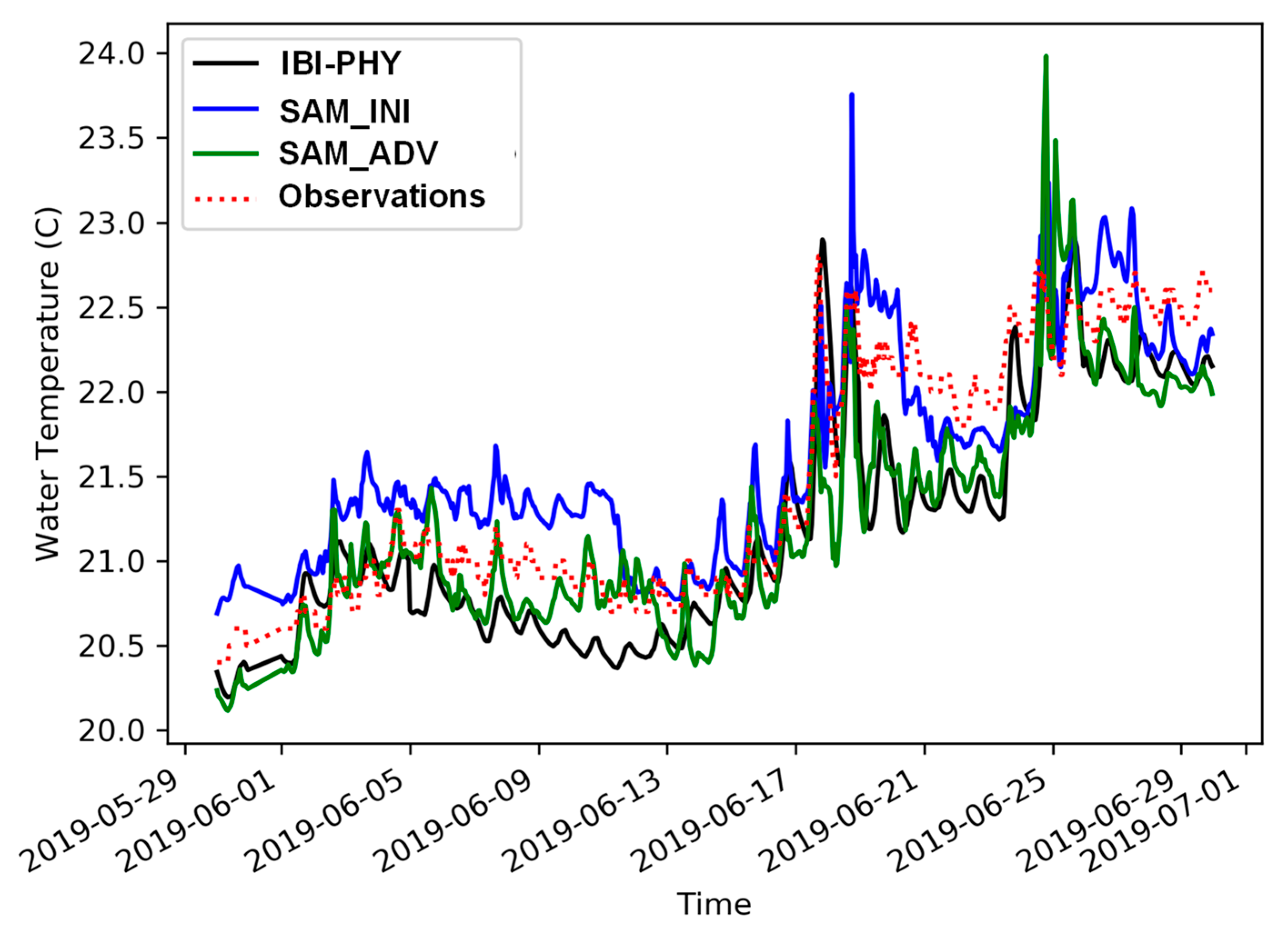
4.1. Impacts in SAMOA Solutions Related to Changes in the OBC Treatment and the Use of a Bulk Formula to Deal with Atmospheric Forcing (SAM_ADV vs. SAM_INI)

This first SAM_INI configuration was carried out based on the SAMOA-1 model set-up after the update of the HARMONIE atmospheric forcing (see Section 3.1). The upgraded SAMOA set-up (SAM_ADV test) related to changes in the OBC treatment and the use of a Bulk formula is further described in Section 3.2.

The error metrics from both SAMOA tests and the IBI_PHY solution are summarized in Table 3. In general, it is seen that SAM_ADV improves considerably the SAM_INI Sea Surface Temperature (SST):

(i)

Bias drop from 0.20 °C (SAM_INI) to −0.03 °C (SAM_ADV), even moderately better than IBI_PHY (0.07 °C).

(ii)

Correlations were close to 0.8 for all three models.

(iii)

IBI_PHY had lower RMS (0.44 °C) than SAM_INI (0.6 °C) and SAM_ADV (0.5 °C)

(iv)

COE for IBI_PHY (0.29) and SAM_ADV (0.21) were similar, substantially higher than SAM_INI (0.07).

At a more detailed level, Figure 4 presents the SST at Gran Canaria coastal buoy. Despite that the three models are able to capture the intradaily cycles, SAM_ADV (green line) and IBI_PHY (black line) show similar trends. Additionally, for the first part of the month, SAM_ADV shows more agreement with the observations than SAM_INI (blue line). However, also note that at the second half of the month, there was a sudden rise in temperatures that only SAM_INI captured (though overestimating it).

Regarding mean sea-level, SAM_INI and SAM_ADV show similar performance, improving considerably IBI_PHY, especially at meso-tidal (GOM, GCA and PAL domains) and macro-tidal environments (BIL, FER, VIG). The three models show very high correlations (close to 0.96); but the RMS is lower (close to 0.05 m) for the SAMOA set-ups, whereas IBI_PHY reaches 0.14 m. The same pattern is also found for the COE: both SAMOA have values close to 0.77, but IBI_PHY does not surpass 0.66.

Sea Surface Salinity (SSS) remains with similar metrics between SAMOAs, not improving the IBI_PHY performance. RMS are identical and the COE is negative at all three. Hence, SAMOA does not add new information on this variable.

Surface currents also exhibit similar metrics amongst the different models. Note though, that at a qualitative assessment level, SAM_ADV has shown more consistency with the IBI_PHY patterns than SAM_INI. These phenomena especially happened at the SAMOA boundaries, where the presence of spurious rim-currents was partially alleviated. The consistency of the SAM_ADV OBC scheme was confirmed with the SAM_H3D test (next Subsection).

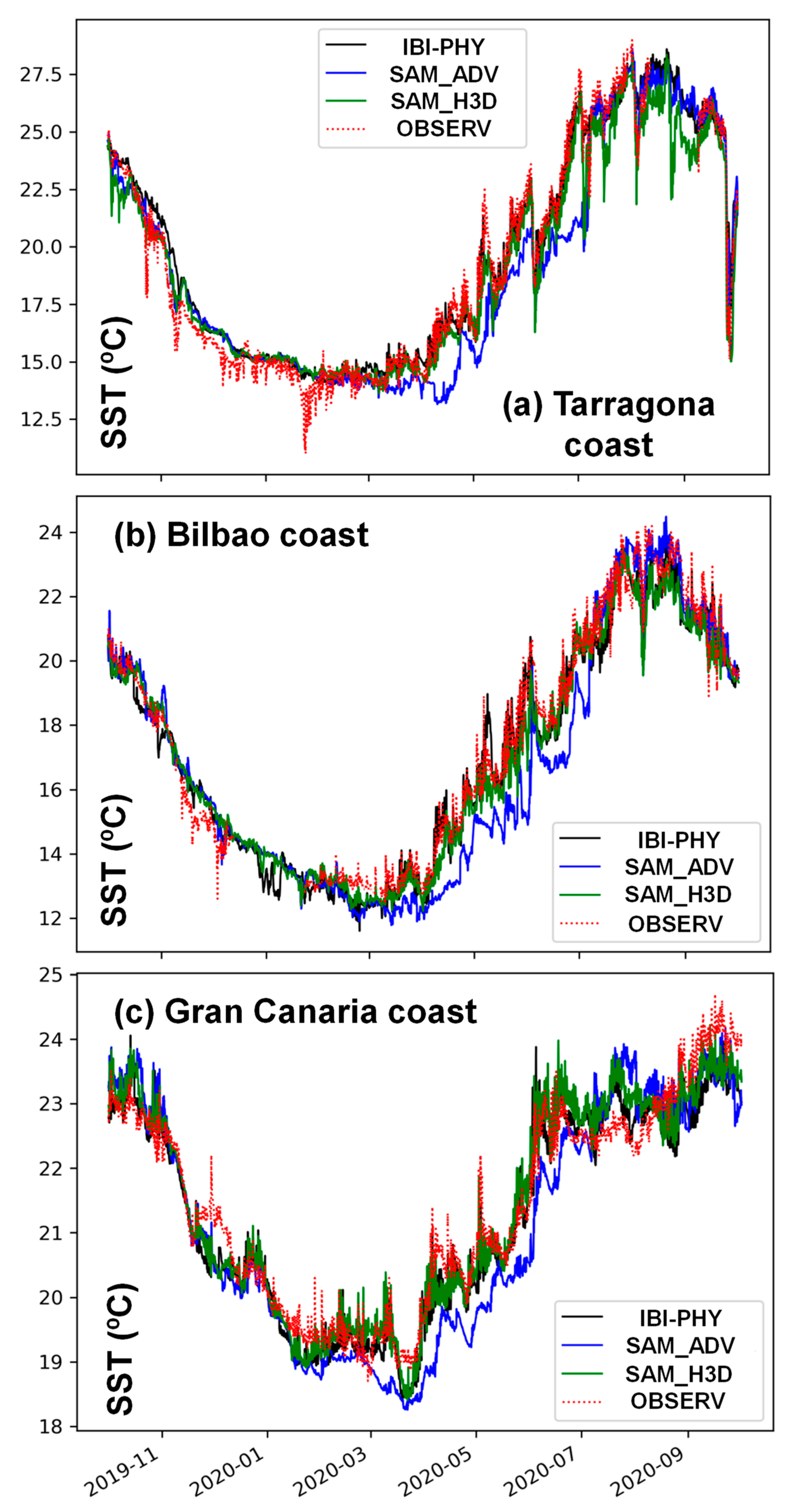
4.2. Impact in the SAMOA Solutions Related to Changes in the Physics and in the Temporal Frequency of the Imposed Data along Boundaries (SAM_H3D vs. SAM_ADV)

As pointed in the previous section, SAM_ADV seemed to enhance coherency between the SAMOA systems and their parent solutions (IBI_PHY). However, differences were still high in some cases, affecting the whole domain and specially along the boundaries. The availability of new hourly-3D CMEMS IBI-MFC products, joint with the upgrade of some physical parametrizations, allowed building the SAM_H3D set-up at 5 systems that were compared with the SAM_ADV and the IBI_PHY parent solution. Their results are summarized in Table 4 and Table 5 and Figure 5, Figure 6 and Figure 7.

Regarding SST (Table 4), lower biases are found in the SAM_H3D (deep water TAR buoy, ALM and GCA) and IBI_PHY (BCN, BIL and coastal TAR buoy). Correlation is close to 0.98 at IBI_PHY and SAM_H3D, slightly higher than for the SAM_ADV case (0.96); pointing the correct capture of the intraday variability. IBI_PHY presents lower RMS (0.65 °C) than SAM_H3D (0.72 °C) and SAM_ADV (0.97 °C). The COE shows good agreement between SAM_H3D (0.83) and IBI_PHY (0.84), whilst SAM_ADV is significantly lower (0.76).

Gran Canaria (GCA) is the system in which SAM_H3D clearly outperforms IBI_PHY and SAM_ADV: (i) the bias is lower (−0.02 °C) than in IBI_PHY (−0.15 °C) and SAM_ADV (−0.31 °C) cases; (ii) SAM_H3D RMS (0.4 °C) is in the same line than IBI_PHY (0.38 °C), and lower than SAM_ADV (0.59 °C).

Error metrics are consistent with the time-series plots (Figure 5), as the model performance between IBI_PHY (black line) and SAM_H3D (green line) are fairly similar at the coastal buoys. Both systems capture the main trends and seasonal changes. However, SAM_ADV (blue line) presented a consistent negative/positive bias in the Winter-Spring/Summer, most probably due to heat-fluxes mismatches at the model domain. Note also that the error metrics between SAM_ADV and SAM_H3D present more agreement at deep waters (closer to the SAMOA domain boundary) than at the coastal locations (far away from the boundaries, heavily influenced by coastal circulation processes and a proper advection scheme).

Surface salinity is improved in Tarragona with the SAMOA solution, though SAM_ADV shows slightly better metrics (−0.13 PSU bias, 0.54 correlation) than SAM_H3D (−0.14 PSU, 0.49) and IBI_PHY (−0.18 PSU, 0.43). At Bilbao and Almería, the error metrics are quite similar for the three models, although SAM_ADV and IBI_PHY moderately outperform SAM_H3D.

As in Section 4.1, SAMOA Sea Level solution outperforms notably IBI_PHY at meso-tidal and macro-tidal environments: the RMS at these two places is significantly lower with SAMOA (0.13 m Bilbao, 0.08 m Gran Canaria) than IBI_PHY (0.27 m Bilbao, 0.12 m Gran Canaria). COE presents important differences (close to 0.9 in SAMOA, whilst IBI_PHY has 0.74 in Bilbao and 0.8 at Gran Canaria).

Sea Level at Barcelona and Tarragona exhibit similar behaviour on the three models. However, at these two domains, IBI_PHY solution exhibits a higher COE (around 0.6) and the long-term metrics underperform both at SAM_ADV and SAM_H3D.

Apart from SST, the most prominent differences at the SAM_H3D are found in the sea surface currents, both at current speed and direction (Table 4). Current direction metrics from SAMOA outperform at deep-water buoys: (i) SAM_H3D (−1.4°) bias is lower than IBI_PHY (−4.6°); (ii) correlation and RMS are also better at SAM_H3D (0.3, 74.2°) than at IBI_PHY (0.27, 84.2°).

Regarding surface current speed at Tarragona deep-water buoy, significant improvement in the correlation can be found (0.35 (SAM_ADV) vs. 0.36 (SAM_H3D) vs. 0.25 (IBI_PHY)). RMS is similar for all three datasets (0.16 vs. 0.18 vs. 0.17, respectively); but the bias is lower in IBI_PHY (0.01 m/s), and higher in SAM_H3D (0.05 m/s) than in SAM_ADV (0.03 m/s).

Tarragona and Gran Canaria are the two SAMOA that have coverage from Radar HF. Hence, special emphasis would be given. Error metrics have been computed at five specific points (Table 5), representative of the area (see their position at subpanels (c) in Figure 6 and Figure 7).

Figure 6 shows the monthly-averaged HF-radar measurements, model results and error metrics in Tarragona during March 2020. In that month, there were four clustered NW inland wind-jets in the first week of the month, reaching hourly wind-speeds up to 20 m/s. From 10th March until the end of the month, the atmospheric conditions were fairly stable, though: wind speed had a mean average close to 3–4 m/s. Note however, that at Figure 6c, even at a monthly-averaged scale, these inland wind-jets are the most remarkable signature.

Both SAMOA systems reproduce the origin and the propagation of wind-jet. But SAM_H3D is the solution that shows more resemblance with the surface HF radar (Figure 6g–i), exhibiting correlations close to 0.5 at the wind-jet influence area. IBI_PHY does not reproduce the wind-jet and it tends to overestimate the Northern Current and General circulation, remaining some influence from circulation features associated to extreme storm events occurred in previous months (i.e., Mediterranean Storm Gloria).

At the Gran Canaria case (Figure 7) there were persistent, but moderate, NE wind speed (lower than 8 m/s, with monthly-averaged values close to 3 m/s). The monthly-averaged HF radar exhibits consistency (Figure 7c) with these wind field conditions. Surface circulation is mainly SW, exhibiting higher values at the South (close to 0.30 m/s) than in the North (around 0.1 m/s). IBI_PHY (Figure 7a) exhibits a clockwise gyre near the Gran Canaria harbour. This eddy is also reproduced in SAM_ADV set-up (Figure 7d–f), but it is not in SAM_H3D (Figure 7g–i).

SAM_ADV overestimates currents at the Southern part of the domain (Figure 7d). Biases at the SAM_H3D boundary are lower than SAM_ADV and even IBI_PHY. Additionally, SAM_H3D exhibit higher correlation at the Southern part of the domain (close to 0.7). Note that in SAM_ADV, the correlation is negative at the central part of the Eastern boundary. These findings are consistent regardless of the measurement devices, as the analysis performed with RadarHF and deep-water buoy observational data denote similar patterns in terms of error metrics.

5. Discussion

In the previous section, the main results were shown from the different SAMOA model set-up tests (SAM_INI, SAM_ADV, SAM_H3D) performed at different coastal and port domains. All the SAMOA simulations were validated with observational data sources for sea level, surface currents, SST and SSS, and compared with its parent solution (IBI_PHY).

The main aim of these SAMOA sensitivity tests is to assess the impacts that potential upgrades in the SAMOA set-up have on its solution at different domains. Once the quality control is performed (i.e., by comparing SAMOA solutions with IBI_PHY solutions, joint with the available observations at each coast/port domain), it can be verified whether the proposed set-up may result in a new operational SAMOA release.

Prior to deciding a new operational SAMOA release, it would be needed to verify if the new solution improves/degrades the control one (and at what level). Furthermore, it is not enough to test the model set-up upgrade in a single SAMOA domain; it is needed to be assessed how the positive impacts extend across the different SAMOA port systems.

Table 6. Summary of the impacts of the SAM_ADV set-up. Performance of SAM_ADV versus the control (SAM_INI) one and the parent solution (IBI_PHY), comparing in those domains where observations are available (for sea level, SST, SSS and surface currents). Legend: (SAM_ADV relative performance with respect to SAM_INI set-up/SAM_ADV relative performance with respect to IBI_PHY). Acronyms to define the relative performance of the proposed set-up: (I *: relevant improvement/I: improvement/S: similar performance/W: mild worsening).

SAMOA System	Sea Level	Surface Currents	SST	SSS
Barcelona (BCN)	(S/W)	-	(W/S)	-
Tarragona (TAR)	(I/I)	(S/S)	(W/W)	(S/S)
Bilbao (BIL)	(S/I *)	(S/S)	(I/S)	(I/I)
Ferrol (FER)	(S/I *)	-	(I */W)	-
Vigo (VIG)	(S/I)	-	-	-
Almería (ALM)	(S/I)	(S/W)	(I */I)	(S/S)
Gran Canaria (GCA)	(S/I *)	-	(I */W)	-
La Gomera (GOM)	(I/I)	-	-	-
St. Cruz Palma (PAL)	(S/I *)	-	-	-
Tenerife (TEN)	-	-	(I */W)	-

summarizes the results of the SAM_INI vs. SAM_ADV and the IBI_PHY parent solution (see SAMOA model set-up descriptions in Section 3.2. and the main validation results in the Section 4.1). In general terms, SAM_ADV improves sea level significantly in respect to IBI_PHY, but remains similar to the SAMOA control run (SAM_INI). The SST simulated with the SAM_ADV set-up improves the SAM_INI one, but the solution is worse than the one from the Copernicus IBI_PHY product. Surface salinity remains similar in all the model solutions, with SAM_ADV outperforming in the Bilbao domain. With respect to surface current speed, a slightly better performance of IBI_PHY is seen in the three cases where observations are available, but both SAMOA experiments outperform the surface current direction; the three solutions may be considered as similar for currents.

The proposed SAMOA SAM_ADV set-up improves notably the Sea Level respect the IBI-MFC solution, especially at meso and macro-tidal environments. The higher spatial resolution of SAMOA systems allows to better capture of the harbour geometry and coastal surroundings, being a plausible explanation of such improvement in terms of sea level. The use of the new COARE bulk formula introduced in the SAM_ADV test improves (significantly) the sea surface temperature metrics with respect to the SAM_INI control one in 5 (4) out of the 7 cases analysed. This significant improvement led SAM_ADV SAMOA set up to be transitioned into operations in October 2019, thus becoming the current (end of 2021) operational set-up.

Improvements in operational systems tend to be incremental. The proposed SAM_H3D configuration enhances the SAM_ADV one in Surface Currents and SST; whereas Sea Level metrics remain similar (see summary of relative performances in

Table 7. Summary of the impacts of the SAM_H3D proposed set-up. Performance of SAM_H3D versus the control (SAM_ADV) one and the parent solution (IBI_PHY), comparing in those domains where observations are available (for sea level, SST, SSS and surface currents). Legend: (SAM_H3D relative performance with respect to SAM_ADV set-up/SAM_H3D relative performance with respect to IBI_PHY). Acronyms to define the relative performance of the proposed set-up: (I *: relevant improvement/I: improvement/S: similar performance/W: mild worsening).

SAMOA System	Sea Level	Surface Currents	SST	SSS
Barcelona (BCN)	(S/W)	-	(I */S)	-
Tarragona (TAR)	(S/W)	(I/I)	(I */I)	(S/I *)
Bilbao (BIL)	(S/I *)	(S/S)	(I */S)	(W/W)
Almería (ALM)	(S/S)	(S/W)	(I/S)	(W/W)
Gran Canaria (GCA)	(S/I *)	(I */I)	(I */I)	-

). SAM_H3D also outperforms IBI_PHY at the following issues: (i) Sea Level in meso-tidal and macro-tidal environments; (ii) Surface current speed correlation and surface current direction; (iii) SST at intermediate and shallow waters (i.e., coastal buoys); (iv) Surface Salinity at Tarragona. The main reasons for this behaviour are discussed below.

First, better surface current correlations at SAM_H3D (respect to SAM_ADV) are related to three factors: (i) tidal-induced currents are correctly nested with the parent solution; (ii) wind-induced currents are better modelled with the COARE 3.6 parametrization; and (iii) SAMOA solutions exhibit more spatial heterogeneity than IBI_PHY. This last issue (heterogeneity) can be partly explained due to SAMOA higher spatial resolution. For instance, the model grid is able to reproduce sharp bathymetric pressure gradients; joint with the atmospheric forcing data that features local orographic constraints.

In this sense, atmospheric forcings are an important cause of the mismatch. SAMOA uses HARMONIE that has a systematically higher wind speed bias than ECMWF: around 1.5 m/s yearly-averaged difference along the coastal and deep waters of Iberian Peninsula, Balearic and Canary Islands. At the inland stations, biases between the two forcings are similar, mostly due to more stations to be assimilated. Moreover, HARMONIE overestimation can increase up to 7 m/s during extreme events, such as the recent Storm Gloria (January 2020) (Sotillo et al., 2021a [47]); whilst ECMWF tend to lower overestimations (close to 3 m/s). Such HARMONIE overestimation is one of the main reasons for the higher bias and RMS at some stations in the SAMOA surface currents, with respect to IBI_PHY.

Wind direction, though, provides a trade-off: whereas ECMWF biases can reach close to 30° at coastal locations, HARMONIE remains more accurate (biases around 10–20°). The higher horizontal resolution of HARMONIE (2.5 km vs. 10 km) is able to solve the orographic constraints, island boundaries and intraday processes (such as sea-breezes) more accurately. For instance, the Tarragona system is prone to wind jets (Grifoll et al., 2016 [48]), mainly constrained by the mountain-ranges close to the coastal fringe. As can be seen in the Tarragona case (Figure 6a), IBI_PHY forced with ECMWF-IFS cannot reproduce the wind jet. ECMWF-IFS coarse resolution (10 km) is not enough for modelling the narrow sharp topographic gradients between the mountain ranges near the Ebro Delta, but HARMONIE does it (see the SAMOA solutions in Figure 6d,g).

Hence, proper current direction is an important remark, especially when tidal-currents act concomitant to wind-induced currents. Errors in the wind direction can lead to wind-induced stresses; that albeit accurate in modulus, incorrectly reinforce/weakens surface currents driven by other physical processes.

IBI_PHY uses CORE bulk formula (Large and Yaeger, 2004 [49]), SAM_ADV the COARE 3.0 (Fairall et al., 2003 [33]), and SAM_H3D the COARE 3.5 (Edson et al., 2013 [39]). Charnock coefficient in COARE 3.5 (and its parametrized surface-drag coefficient) is lower for moderate winds than in COARE 3.0 (Brodeau et al., 2017 [50]). In COARE 3.0, Charnock coefficient is set to constant (0.011) at wind speeds from 0 to 10 m/s; whereas in COARE 3.5, Charnock is set to 0.006 until 6 m/s. Due to the systematic overestimation of the HARMONIE wind fields, the reduction of the wind-stresses can be a factor for the enhancement of SAM_H3D surface currents metrics, especially in correlation and general bias, when moderate wind conditions prevail.

Another difference between SAM_ADV and SAM_H3D is that the gustiness parameter is lower in COARE 3.5 than in the former release; and that may boost surface stresses at extreme wind regimes. Gustiness effects are not included in CORE, that may be a secondary factor for better IBI_PHY RMS metrics (ECMWF atmospheric forcings influence, being a primary one). Nonetheless, CORE drag coefficients tend to be higher than COARE at moderate wind speeds; and vice versa, from moderate to high winds (Pelletier et al., 2018 [51]). Further research in air-sea interaction would shed some light on this key issue.

SAM_H3D is the solution that shows more resemblance with the spatial signature from surface HF radar (Figure 6 and Figure 7). Note however, that both SAMOA solutions are heavily constrained by the IBI_PHY solution. For instance, the spurious SW fluxes at the Eastern corner at the Tarragona model (Figure 6) are mainly due to the IBI parent solution. Eddies in the boundaries and corners, such as the clockwise one close to the Southern corner can be also problematic, especially when IBI patterns are unrealistic. The SAM_H3D nesting ensures mass and momentum conservation from the parent to child grids, but errors in the former can be easily propagated.

This latter phenomenon may partly explain the low predictive skill in the Almería system, both with IBI_PHY and SAMOA. A possible reason may be transient spurious mesoscale structures in IBI_PHY at Cabo de Gata (Figure 2). High surface current direction bias is found at the deep-water EXT buoy (almost 30°, in comparison with the 3° bias found when compared at the Bilbao or Tarragona EXT buoys). Note that these errors in direction are inherited from the parent solution (IBI_PHY), suggesting that the transport direction is incorrect. This phenomenon also affects both heat and salinity fluxes. Hence, a plausible solution to minimize undesired influences related to spurious dynamic features identified in the IBI_PHY parent solution may be to expand the SAMOA coastal domain, fixing the SAMOA boundaries outside of the areas where such spurious structures are favoured in the IBI_PHY solution; then generating a SAMOA intrinsic solution, less constrained by the limited-area domain and the IBI_PHY data imposed as boundary condition.

Regarding SST, the enhancement of SAM_H3D solution may be due to three factors: (i) better characterization of the heat fluxes with COARE 3.5; (ii) consistent circulation fields and (iii) the use of HSIMT-TVD advection scheme for passive tracers. Despite that SAMOA does not have data assimilation, the one-year metrics are close, or even better (at some cases) than IBI_PHY. Note that the Copernicus Regional System counts with a data assimilation scheme. Then, satellite SST fields and in-situ profiles data are assimilated in the IBI_PHY analyses.

In this sense, Gran Canaria highlights the role of coastal circulation in shallow-depths heat fluxes, as the enhancements of the circulation fields are consistent with SST ones. The RMS is lower in IBI_PHY than SAMOA, though; most probably due to the radiation forcings (be it short or long-wave), that have higher variability in HARMONIE than ECMWF.

SAMOA significantly improves the sea level, especially in those areas with meso and macro-tides. There is no important difference between SAM_ADV and SAM_H3D, suggesting that the main improvements come from the increase of horizontal resolution, that lead to better capture of the harbour geometry and coastal surroundings. Water mass fluxes and piling-up effects are better reproduced.

However, the performance is substantially lower at the Barcelona and Tarragona cases (as shown in the Table 3 metrics), in which all the three models require further assessment on two aspects:

(i)

Inclusion of low frequency astronomical constituents, such as the solar semi-annual (Ssa) and solar annual (Sa) constituents. For these two specific systems, low-frequency constituents have an equivalent order of magnitude than higher frequency harmonics: for instance, in Tarragona, the sum of the amplitudes of the M2 (3.97 cm) and K1 (3.71 cm) are close to the SA value (7.21 cm) (Pérez-Gómez, 2014 [42]). Low-frequency constituents require long-term observations for its correct estimation; and this remains a main shortcoming for their inclusion in operational models.

(ii)

The non-tidal residual term is not properly modelled in IBI_PHY at specific synoptic conditions, due to no inclusion of the whole Mediterranean basin subinertial transport. The IBI_PHY storm-surge solution for the recent storm Gloria was analysed in Pérez-Gómez et al., 2021 [52], then identifying a persistent underestimation of the positive surge. Such underestimation was mainly related to the fact that IBI system does not include barotropic mass-transport from the Eastern Mediterranean subbasin towards the Western Mediterranean one. Correction for this misbalance in the MSLP-driven transports between the Mediterranean sub-basins is in the IBI-MFC roadmap, and it is expected to be overcome in forthcoming IBI_PHY operational releases.

Wave-driven currents are another point in which SAMOA will devote further efforts. At present (late 2021), the Copernicus IBI_PHY solution is one-way coupled with the IBI-WAV system (based on the WAM (WAMDI Group, 1988 [53]) spectral wave model) by adding (i) the Stokes drift, (ii) wave-induced mixing and (iii) wind drag coefficients formulas based on the sea-state. This addition may be particularly important during wave storms, as suggested in Sotillo et al., 2021a [47] and Lorente et al., (2021) [54]. Current developments of the SAMOA system, developed within the EuroSea Project, are going in the same direction, with strong focus on the local processes beneath intermediate and shallow waters.

Same focus on local coastal processes, that has become the leitmotif of the SAMOA forecasting system, will also be taken on improving the land-sea connection. Proper modelling of salinity fluxes require operational run-off discharge products, such as the one analysed in this issue (Sotillo et al., 2021b [55]), rather than climatological values. All these improvements, albeit ambitious, represent a clear SAMOA roadmap for the coming years. Moreover, as suggested in the case of Gran Canaria (i.e., SST improves when surface currents do it), the synergistic gain from addressing all of them, would enhance the predictive skill of SAMOA operational products at an integrated level.

6. Conclusions

6.1. Assessment of the SAMOA Coastal Forecasting Service Upgrades

The Puertos del Estado SAMOA coastal and port ocean forecast service has delivered operational ocean forecast products to Spanish Port Authorities since 01/2017. The service provides daily forecasts of sea-level, circulation, temperature and salinity fields at horizontal resolution that range from 350 m (Coastal domains) to 70 m (Port domains). The system was successfully implemented at nine ports in the SAMOA-1 project (2014–2017); and it was expanded, improving the model set-up, to 31 ports at the end of SAMOA-2 project (2018–2021).

This contribution has assessed the incremental upgrades that have been developed in the SAMOA system from 2018 to 2021. In chronological order, it has been tested (at different ports) the following three main set-ups:

(i)

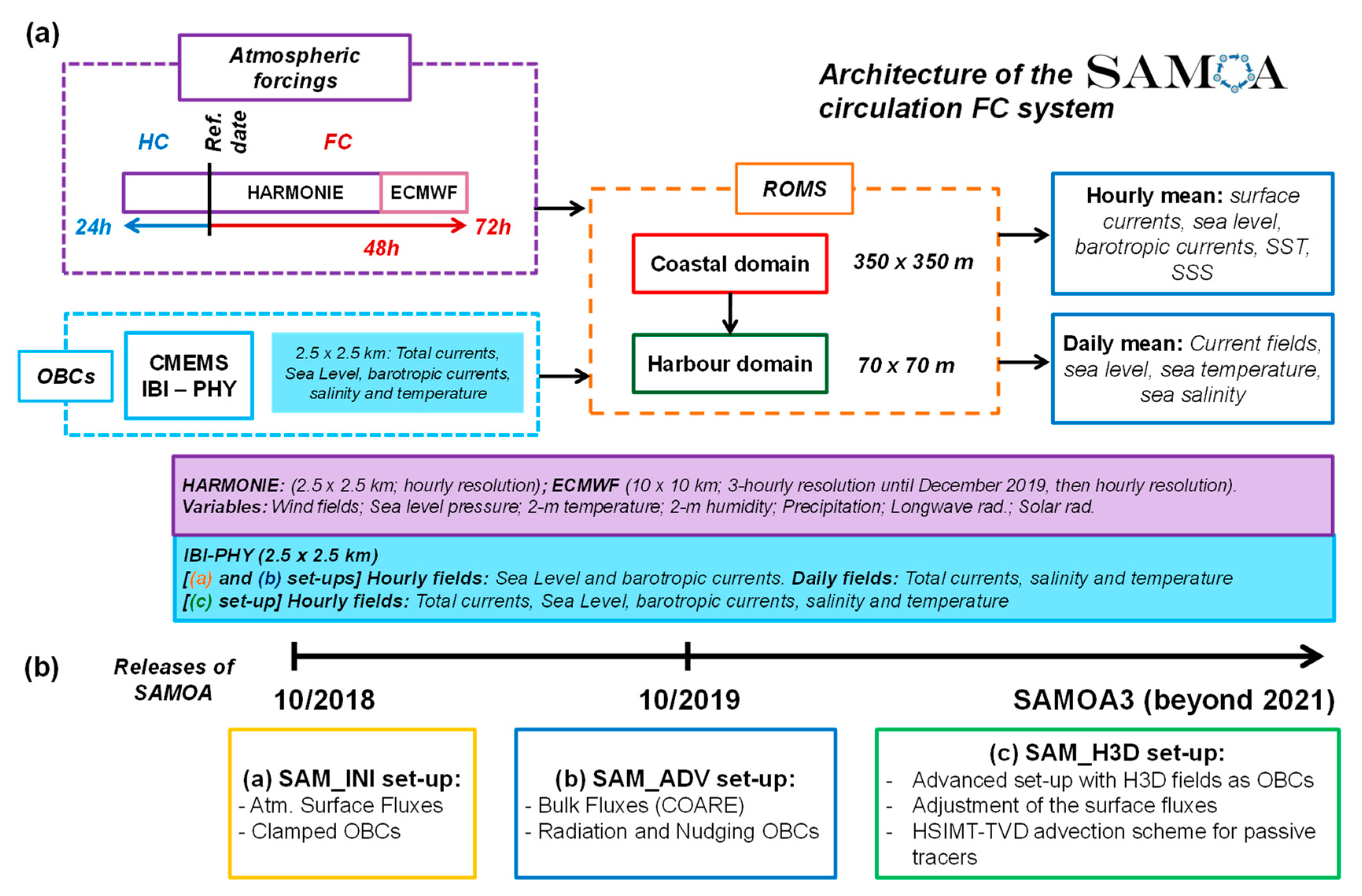
The SAM_INI configuration, analogous to the one used in SAMOA-1, but substituting the former AEMET HIRLAM atmospheric forcing by the new HARMONIE 2.5 km forcing data.

(ii)

The SAM_ADV set-up, focused on upgrading the open boundary condition scheme treatment and the computation of surface atmosphere-ocean fluxes through the COARE 3.0 bulk formula.

(iii)

The SAM_H3D set-up, in which it is proposed (a) the use of the hourly-3D IBI-MFC forecast dataset, (b) the update of the bulk formula for surface fluxes (COARE 3.5), (c) the use of a new advection scheme (HSIMT-TVD) for passive tracers and (d) the reduction of the wind-stresses due to the effect of surface currents.

The protocol proposed to assess these SAMOA model set-up upgrades focuses on evaluating in the Spanish ports the simulation of ocean variables (typically, the sea level, currents, surface temperature and salinity), validating them with available in-situ and remote-sensed observations (from tide gauges, mooring buoys and HF Radar stations). To check model sensitivities, as well as to evaluate the potential added value related to the proposed modifications, each SAMOA model test run is always compared with a control SAMOA run (i.e., the operational version of the SAMOA system at the time of the test), and with the CMEMS IBI_PHY parent solution.

Applying this protocol, it was demonstrated that:

(i)

The three proposed SAMOA tests improve notably the simulation of sea level with respect to the IBI_PHY parent solution, especially at meso- and macro-tidal environments. The SAMOA higher spatial resolution allows to better capture of the harbour geometry and coastal surroundings.

(ii)

The use of the COARE bulk formula (introduced in the SAM_ADV set-up) improved sea surface temperature (SST) metrics respect to SAM_INI; but SAM_H3D outperforms SAM_ADV and the skill is close to the IBI_PHY solution. This SAM_H3D improvement in SST can be explained by (a) improvements in the surface fluxes physics, (b) the use of HSIMT-TVD for passive tracers and especially (c) the overall improvement of the surface circulation fields.

(iii)

This improvement of the circulation fields arises from two factors: (a) the SAM_H3D nesting ensures mass and momentum conservation from the IBI_PHY parent solution (hourly updated) to the SAMOA child grids along boundaries; and (b) SAM_H3D benefits from the high-resolution HARMONIE forcing. These two factors allow proper modelling of joint tidal and wind-induced currents. Consequently, local effects such as in-land wind-jets (case of Tarragona HF radar), and those influenced by topographic gradients exhibit good metrics in SAM_H3D, even slightly better than in IBI_PHY. At the Gran Canaria case, SAM_H3D is the model solution that shows more resemblance with the spatial signature from surface HF radar. However, the Almería case also highlights how the SAM_H3D nesting scheme can propagate errors or spurious circulation features from IBI_PHY into the SAMOA solution.

(iv)

Finally, this contribution summarizes the impact of the incremental model upgrades performed in the SAMOA operational circulation system since 2018. Indeed, two of the SAMOA model set-ups here shown (SAM_INI and SAM_ADV) have been the base for the last two operational SAMOA releases (launched in October 2018 and October 2019, respectively). The SAM_ADV model configuration is the current SAMOA operational set-up, but it is expected to be upgraded in 2022 by the also here tested SAM_H3D one. This contribution demonstrates that the proposed SAM_H3D configuration enhances the current SAMOA solution, especially in terms of surface currents and SST.

6.2. Recommendations for Coastal Forecasting Services and Future SAMOA Perspectives

This contribution has presented the SAMOA circulation system as a downstream service that benefits from Copernicus regional products. The authors recommend the use of products that ensure proper nesting between the parent solution and the local application. In this sense, the use of the hourly-3D IBI-MFC forecast dataset has contributed to improve the circulation and sea temperature fields (as shown in the SAM_H3D set-up). It has been shown, that the error metrics decrease when the boundary conditions have hourly-averaged resolution (be it sea-level, currents, sea temperature and salinity). This product ensures more consistency with the parent solution than the previous SAMOA releases (hourly-averaged sea-level and barotropic currents; but daily-averaged total currents, temperature and salinity).

High resolution atmospheric forcings and the proper air-sea parameterizations have also proven to be relevant in modelling local processes, such as wind-jets. The COARE 3.5 bulk-formula (implemented in SAM_H3D) has shown better skill than COARE 3.0. The HSIMT-TVD scheme contributed to improve sharp gradients in the sea surface temperature solution.

This research has also identified the following future perspectives for the development of SAMOA:

(i)

To improve the modelling of air-sea interaction processes, with focus on surface stresses and heat fluxes.

(ii)

To expand the coastal domains, with the aim of generating intrinsic solutions that are less dependent on limitations from the parent solution (such as its inability to reproduce accurately certain topographic gradients, due to its coarser horizontal resolution).

(iii)

To include wave-driven effects such as (a) the Stokes drift interaction with the currents, (b) wave-induced mixing parameterizations and (c) wind drag coefficients formulas based on the sea-state.

(iv)

To include low-frequency astronomical tide constituents. These low-frequency harmonics are especially relevant in those SAMOA systems located at the Western Mediterranean sub-basin.

(v)

To verify and to correct (if needed) the subinertial transport at specific SAMOA systems, then enhancing the forecast skill under certain synoptic conditions.

(vi)

To couple the SAMOA systems with operational coastal run-off discharge systems.

The joint action of these synergistic developments will reinforce SAMOA leitmotif: a downstream service, fed by Copernicus regional products, that enhances predictive capabilities on local coastal processes at Spanish Port zones.

References

1. European Global Observing Systems (EuroGOOS). Available online: http://eurogoos.eu/ (accessed on 18 January 2022).
2. Schiller, A.; Mourre, B.; Drillet, Y.; Brassington, G. An overview of operational oceanography. In New Frontiers in Operational Oceanography; Chassignet, E., Pascual, A., Tintoré, J., Verron, J., Eds.; GODAE OceanView: Madrid, Spain, 2018; pp. 1–26. [Google Scholar] [CrossRef] [Green Version]
3. Davidson, F.; Alvera-Azcárate, A.; Barth, A.; Brassington, G.B.; Chassignet, E.P.; Clementi, E.; De Mey-Frémaux, P.; Divakaran, P.; Harris, C.; Hernandez, F.; et al. Synergies in Operational Oceanography: The Intrinsic Need for Sustained Ocean Observations. Front. Mar. Sci. 2019, 6, 450. [Google Scholar] [CrossRef] [Green Version]
4. De Mey-Frémaux, P.; Ayoub, N.; Barth, A.; Brewin, R.; Charria, G.; Campuzano, F.; Ciavatta, S.; Cirano, M.; Edwards, C.A.; Federico, I.; et al. Model-Observations Synergy in the Coastal Ocean. Front. Mar. Sci. 2019, 6, 436. [Google Scholar] [CrossRef] [Green Version]
5. EU EuroStat. EuroStat Explaining Statistics: Maritime Ports Freight and Passenger Statistics. 2017. Available online: http://ec.europa.eu/eurostat/statistics-explained/index.php/Maritime_ports_freight_and_passenger_statistics (accessed on 18 January 2022).
6. Álvarez Fanjul, E.; Sotillo, M.G.; Pérez, B.; García-Valdecasas, J.M.; Pérez, S.; Lorente, P.; Rodríguez-Dapena, A.; Martínez, I.; Luna, Y.; Padorno, E.; et al. Operational oceanography at the service of the ports. In New Frontiers in Operational Oceanography; Chassignet, E., Pascual, A., Tintoré, J., Verron, J., Eds.; GODAE OceanView: Madrid, Spain, 2018; pp. 729–736. [Google Scholar] [CrossRef] [Green Version]
7. Sotillo, M.G.; Cerralbo, P.; Lorente, P.; Grifoll, M.; Espino, M.; Sanchez-Arcilla, A.; Álvarez-Fanjul, E. Coastal ocean forecasting in Spanish ports: The SAMOA operational service. J. Oper. Oceanogr. 2019, 13, 37–54. [Google Scholar] [CrossRef]
8. Lellouche, J.-M.; Greiner, E.; Le Galloudec, O.; Garric, G.; Regnier, C. Recent updates to the Copernicus Marine Service global ocean monitoring and forecasting real-time 1/12° high-resolution system. Ocean Sci. 2018, 14, 1093–1126. [Google Scholar] [CrossRef] [Green Version]
9. Lellouche, J.-M.; Le Galloudec, O.; Drévillon, M.; Régnier, C.; Greiner, E.; Garric, G.; Ferry, N.; Desportes, C.; Testut, C.-E.; Bricaud, C.; et al. Evaluation of global monitoring and forecasting systems at Mercator Océan. Ocean Sci. 2013, 9, 57–81. [Google Scholar] [CrossRef] [Green Version]
10. Liu, H.; Lin, P.; Zheng, W.; Luan, Y.; Ma, J.; Ding, M.; Mo, H.; Wan, L.; Ling, T. A global eddy-resolving ocean forecast system in China—LICOM Forecast System (LFS). J. Oper. Oceanogr. 2021, 14, 2781–2799. [Google Scholar] [CrossRef]
11. Bell Michael, J.; Lefebvre, M.; Le Traon, P.Y.; Smith, N.; Wilmer-Becker, K. GODAE The Global Ocean Data Assimilation Experiment. Oceanography 2009, 22, 14–21. [Google Scholar] [CrossRef]
12. Bell, M.J.; Schiller, A.; Le Traon, P.-Y.; Smith, N.R.; Dombrowsky, E.; Wilmer-Becker, K. An introduction to GODAE OceanView. J. Oper. Oceanogr. 2015, 8 (Suppl. 1), s2–s11. [Google Scholar] [CrossRef]
13. Tonani, M.; Balmaseda, M.; Bertino, L.; Blockley, E.; Brassington, G.; Davidson, F.; Drillet, Y.; Hogan, P.; Kuragano, T.; Lee, T.; et al. Status and future of global and regional ocean prediction systems. J. Oper. Oceanogr. 2015, 8 (Suppl. 2), s201–s220. [Google Scholar] [CrossRef] [Green Version]
14. Copernicus Marine Environmental Monitoring Service (CMEMS). Available online: http://marine.copernicus.eu/ (accessed on 18 January 2022).
15. Le Traon, P.Y.; Reppucci, A.; Alvarez Fanjul, E.; Aouf, L.; Behrens, A.; Belmonte, M.; Bentamy, A.; Bertino, L.; Brando, V.E.; Kreiner, M.B.; et al. From observation to information and users: The Copernicus Marine service perspective. Front. Mar. Sci. 2019, 6, 234. [Google Scholar] [CrossRef] [Green Version]
16. Capet, A.; Fernández, V.; She, J.; Dabrowski, T.; Umgiesser, G.; Staneva, J.; Mészáros, L.; Campuzano, F.; Ursella, L.; Nolan, G.; et al. Operational Modeling Capacity in European Seas—An EuroGOOS Perspective and Recommendations for Improvement. Front. Mar. Sci. 2020, 7, 129. [Google Scholar] [CrossRef] [Green Version]
17. Sotillo, M.G.; Cailleau, S.; Lorente, P.; LeVier, B.; Aznar, R.; Reffray, G.; Amo-Baladrón, A.; Chanut, J.; Benkiran, M.; Alvarez-Fanjul, E. The MyOcean IBI Ocean Forecast and Reanalysis Systems: Operational products and roadmap to the future Copernicus Service. J. Oper. Oceanogr. 2015, 8, 63–79. [Google Scholar] [CrossRef]
18. Aznar, R.; Sotillo, M.G.; Cailleau, S.; Lorente, P.; Levier, B.; Amo-Baladrón, A.; Reffray, G.; Álvarez-Fanjul, E. Strengths and weaknesses of the CMEMS forecasted and reanalyzed solutions for the Iberia–Biscay–Ireland (IBI) waters. J. Mar. Syst. 2016, 159, 1–14. [Google Scholar] [CrossRef]
19. Kourafalou, V.H.; De Mey, P.; Staneva, J.; Ayoub, N.; Barth, A.; Chao, Y.; Cirano, M.; Fiechter, J.; Herzfeld, M.; Kurapov, A.; et al. Coastal Ocean Forecasting: Science foundation and user benefits. J. Oper. Oceanogr. 2015, 8 (Suppl. 1), s147–s167. [Google Scholar] [CrossRef]
20. Sotillo, M.G.; Álvarez-Fanjul, E.; Castanedo, S.; Abascal, A.J.; Menendez, J.; Emelianov, M.; Olivella, R.; García-Ladona, E.; Ruiz-Villarreal, M.; Conde, J.; et al. Towards an operational system for oil-spill forecast over Spanish waters: Initial developments and implementation test. Mar. Pollut. Bull. 2008, 56, 686–703. [Google Scholar] [CrossRef]
21. Sánchez-Garrido, J.C.; García-Lafuente, J.; Álvarez-Fanjul, E.; Sotillo, M.G.; de los Santos, F.J. What does cause the collapse of the Western Alboran Gyre? Results of an operational ocean model. Prog. Oceanogr. 2013, 116, 142–153. [Google Scholar] [CrossRef]
22. Sotillo, M.G.; Amo-Baladrón, A.; Padorno, E.; Garcia-Ladona, E.; Orfila, A.; Rodríguez-Rubio, P.; Conti, D.; Jiménez Madrid, J.A.; de los Santos, F.J.; Álvarez Fanjul, E. How is the Surface Atlantic water inflow through the Gibraltar Strait forecasted? A lagrangian validation of operational oceanographic services in the Alboran Sea and the Western Mediterranean. Deep. Sea Res. Part II Top. Stud. Oceanogr. 2016, 133, 100–117. [Google Scholar] [CrossRef] [Green Version]
23. PdE Opendap Catalogue. Available online: https://opendap.puertos.es/thredds/catalog.html (accessed on 18 January 2022).
24. PdE PORTUS Ocean Monitoring & Forecasting System. Available online: https://portus.puertos.es/ (accessed on 18 January 2022).
25. De Dominicis, M.; Pinardi, N.; Zodiatis, G.; Lardner, R. MEDSLIK-II, a Lagrangian marine surface oil spill model for short-term forecasting–Part 1: Theory. Geosci. Model Dev. 2013, 6, 1851–1869. [Google Scholar] [CrossRef] [Green Version]
26. European Union. Directive (EU) 2019/883 of the European Parliament and of the Council of 17 April 2019 on port reception facilities for the delivery of waste from ships, amending Directive 2010/65/EU and repealing Directive 2000/59/EC. Rom. J. Intell. Prop. L. 2019, 151, 116–142. [Google Scholar]
27. Shchepetkin, A.; McWilliams, J.C. The regional oceanic modeling system (ROMS): A split-explicit, free-surface, topography-following-coordinate oceanic model. Ocean Model. 2005, 9, 347–404. [Google Scholar] [CrossRef]
28. ROMS Model Website. Available online: http://www.myroms.org/ (accessed on 18 January 2022).
29. Ryan, A.G.; Regnier, C.; Divakaran, P.; Spindler, T.; Mehra, A.; Smith, G.C.; Davidson, F.; Hernandez, F.; Maksymczuk, J.; Liu, Y. GODAE OceanView Class 4 forecast verification framework: Global ocean inter-comparison. J. Oper. Oceanogr. 2015, 8 (Suppl. 1), s98–s111. [Google Scholar] [CrossRef]
30. Lorente, P.; Sotillo, M.G.; Amo-Baladrón, A.; Aznar, R.; Levier, B.; Aouf, L.; Dabrowski, T.; Pascual, A.; Reffray, G.; Dalphinet, A.; et al. The NARVAL Software Toolbox in Support of Ocean Models Skill Assessment at Regional and Coastal Scales. In Computational Science—ICCS 2019, Proceedings of the 19th International Conference, Faro, Portugal, 12–14 June 2019; Springer: Cham, Switzerland, 2019; Part IV. [Google Scholar] [CrossRef]
31. Bengtsson, L.; Andrae, U.; Aspelien, T.; Batrak, Y.; Calvo, J.; De Rooy, W.; Gleeson, E.; Hansen-Sass, B.; Homleid, M.; Hortal, M.; et al. The HARMONIE-AROME model configuration in the ALADIN-HIRLAM NWP system. Mon. Weather Rev. 2017, 145, 1919–1935. [Google Scholar] [CrossRef]
32. ECMWF, Evolution of the IFS Cycle. 2019. Available online: https://www.ecmwf.int/en/forecasts/documentation-and-support/changes-ecmwf-model (accessed on 9 June 2021).
33. Fairall, C.W.; Bradley, E.F.; Hare, J.E.; Grachev, A.A.; Edson, J.B. Bulk parameterization of air–sea fluxes: Updates and verification for the COARE algorithm. J. Clim. 2003, 16, 571–591. [Google Scholar] [CrossRef]
34. Flather, R.A. A tidal model of the northwest European continental shelf. Mem. Soc. R. Sci. Liege 1976, 6, 141–164. [Google Scholar]
35. Chapman, D.C. Numerical Treatment of Cross-Shelf Open Boundaries in a Barotropic Coastal Ocean Model. J. Phys. Oceanogr. 1985, 15, 1060–1075. [Google Scholar] [CrossRef] [Green Version]
36. Mason, E.; Molemaker, J.; Shchepetkin, A.; Colas, F.; McWilliams, J.C.; Sangrà, P. Procedures for offline grid nesting in regional ocean models. Ocean Model. 2010, 35, 1–15. [Google Scholar] [CrossRef]
37. Marchesiello, P.; McWilliams, J.C.; Shchepetkin, A.F. Open boundary conditions for long-term integration of regional oceanic models. Ocean Model. 2001, 3, 1–20. [Google Scholar] [CrossRef]
38. Wu, H.; Zhu, J. Advection scheme with 3rd high-order spatial interpolation at the middle temporal level and its application to saltwater intrusion in the Changjiang Estuary. Ocean Model. 2010, 33, 33–51. [Google Scholar] [CrossRef]
39. Edson, J.B.; Jampana, V.; Weller, R.A.; Bigorre, S.P.; Plueddemann, A.J.; Fairall, C.; Miller, S.D.; Mahrt, L.; Vickers, D.; Hersbach, H. On the Exchange of Momentum over the Open Ocean. J. Phys. Oceanogr. 2013, 43, 1589–1610. [Google Scholar] [CrossRef] [Green Version]
40. Álvarez Fanjul, E.; de Alfonso, M.; Ruiz, M.I.; López, J.D.; Rodriguez, I. Real time monitoring of Spanish coastal waters: The deep water network. In Elsevier Oceanography Series; Elsevier: Amsterdam, The Netherlands, 2003; Volume 69, pp. 398–402. [Google Scholar]
41. Alfonso, M.; Lopez, J.D.; Alvarez, E.; Ruiz, M.I. Real time buoy data quality control and exploitation. In Proceedings of the The Fifth COPRI International Conference on Ocean Wave Measurement and Analysis (WAVES), Madrid, Spain, 3–7 July 2005; Coasts, Oceans, Ports, and Rivers Institute, American Society of Civil Engineers: Madrid, Spain, 2005. [Google Scholar]
42. Pérez Gómez, B. Design and Implementation of an Operational Sea Level Monitoring and Forecasting System for the Spanish Coast. Ph.D. Thesis, Cantabria University, Santander, Spain, 2014; 242p. [Google Scholar]
43. Roarty, H.; Cook, T.; Hazard, L.; Doug, G.; Harlan, J.; Cosoli, S.; Wyatt, L.; Álvarez-Fanjul, E.; Terrill, E.; Otero, M.; et al. The Global High Frequency Radar Network. Front. Mar. Sci. 2019, 6, 164. [Google Scholar] [CrossRef]
44. Legates, D.R.; McCabe, G.J. Evaluating the use of ‘goodness-of-fit’ measures in hydrologic and hydroclimatic model validation. Water Resour. Res. 1999, 35, 233–241. [Google Scholar] [CrossRef]
45. Legates, D.R.; McCabe, G.J. A refined index of model performance: A rejoinder. Int. J. Climatol. 2013, 33, 1053–1056. [Google Scholar] [CrossRef]
46. Murphy, A.H. Skill Scores Based on the Mean Square Error and Their Relationships to the Correlation Coefficient. Mon. Weather Rev. 1988, 116, 2417–2424. [Google Scholar] [CrossRef]
47. Sotillo, M.G.; Mourre, B.; Mestres, M.; Lorente, P.; Aznar, R.; García-León, M.; Liste, M.; Santana, A.; Espino, M.; Álvarez-Fanjul, E. Evaluation of the operational CMEMS and coastal downstream ocean forecasting services during the storm Gloria (January 2020). Front. Mar. Sci. 2021, 8, 300. [Google Scholar] [CrossRef]
48. Grifoll, M.; Navarro, J.; Pallares, E.; Ràfols, L.; Espino, M.; Palomares, A. Ocean–atmosphere–wave characterisation of a wind jet (Ebro shelf, NW Mediterranean Sea). Nonlinear Processes Geophys. 2016, 23, 143–158. [Google Scholar] [CrossRef] [Green Version]
49. Large, W.G.; Yeager, S.G. Diurnal to decadal global forcing for ocean and sea-ice models: The data sets and flux climatologies, NCAR Technical Note. Natl. Cent. Atmos. Res. 2004, 11, 324–336. [Google Scholar]
50. Brodeau, L.; Barnier, B.; Gulev, S.K.; Woods, C. Climatologically significant effects of some approximations in the bulk parameterizations of turbulent air–sea fluxes. J. Phys. Oceanogr. 2017, 47, 5–28. [Google Scholar] [CrossRef] [Green Version]
51. Pelletier, C.; Lemarié, F.; Blayo, E. Sensitivity analysis and metamodels for the bulk parametrization of turbulent air–sea fluxes. Q. J. R. Meteorol. Soc. 2018, 144, 658–669. [Google Scholar] [CrossRef] [Green Version]
52. Pérez-Gómez, B.; García-León, M.; García-Valdecasas, J.; Clementi, E.; Aranda, C.M.; Pérez-Rubio, S.; Masina, S.; Coppini, G.; Molina-Sánchez, R.; Muñoz-Cubillo, A.; et al. Understanding Sea Level Processes During Western Mediterranean Storm Gloria. Front. Mar. Sci. 2021, 8, 647437. [Google Scholar] [CrossRef]
53. WAMDI Group. The WAM model—A third generation ocean wave prediction model. J. Phys. Oceanogr. 1988, 18, 1775–1810. [Google Scholar] [CrossRef] [Green Version]
54. Lorente, P.; Lin-Ye, J.; García-León, M.; Reyes, E.; Fernandes, M.; Sotillo, M.G.; Espino, M.; Ruiz, M.I.; Gracia, V.; Perez, S.; et al. On the Performance of High Frequency Radar in the Western Mediterranean During the Record-Breaking Storm Gloria. Front. Mar. Sci. 2021, 8, 205. [Google Scholar] [CrossRef]
55. Sotillo, M.G.; Campuzano, F.; Guihou, K.; Lorente, P.; Olmedo, E.; Matulka, A.; Santos, F.; Amo-Baladrón, A.; Novellino, A. River Freshwater Contribution in Operational Ocean Models along the European Atlantic Façade: Impact of a New River Discharge Forcing Data on the CMEMS IBI Regional Model Solution. J. Mar. Sci. Eng. 2021, 9, 401. [Google Scholar] [CrossRef]
Figure 1. 3 Example of Port user-oriented viewing capability through the SAMOA CMA environmental dashboard: (a) 3-days forecast information for wind, waves and currents at Algeciras Bay; Depicted maximum forecasted values and coloured end-user alert symbols (green-yellow-red) following specific user-customized alert thresholds at location of interest for the Port operations; (b): Map of SAMOA high-resolution forecasted surface current field in nearby waters of the Bilbao Port. (c) Example of Oil spill forecast in front of Barcelona Port. Outputs from the PdE Oil Spill forecast service using SAMOA high resolution forecasted currents.
Jmse 10 00149 g001
Figure 2. SAMOA Coastal/Port circulation forecast systems in operations. Green dots: Operational models systems developed within SAMOA1 (2014–2017). Red dots: Operational model systems developed within SAMOA2 (2018–2021). Bathymetry (in meters) is depicted. Note that systems in the Canary Islands are shown in the bottom left corner box (SW limit: 18.5° W, 27.5° N; NE limit: 13.2° W, 29.5° N).
Jmse 10 00149 g002
Figure 3. Architecture of the SAMOA circulation forecast system. (a) Operational scheme, detailing (i) input data sources, including atmospheric forcing and the ocean solution imposed at the Open Boundary Conditions (OBCs), (ii) the numerical core (ROMS) with domain organization, and (iii) delivered products. (b) SAMOA Operational Releases: The timeline shows main releases of this service since 2018 and their most prominent changes. Please note that the acronyms SAM_INI, SAM_ADV and SAM_H3D will be used throughout the text, to name the different model set-up experiments. Likewise with IBI_PHY (the SAMOA parent solution).
Jmse 10 00149 g003
Figure 4. Observed and modelled Sea Surface Temperature (SST) at Gran Canaria PdE EXT mooring buoy (see location in Table 2) in June 2019. Units in Celsius degrees. The dotted red line represents the observations; the solid black line is the parent solution (CMEMS IBI_PHY); the solid blue line is the initial SAMOA set-up (SAM_INI); and the solid green line represents the SAMOA solution obtained with the advanced set-up (SAM_ADV).
Jmse 10 00149 g004
Figure 5. Observed and modelled Sea Surface Temperature (SST) at 3 coastal buoys. (a): Tarragona coast. (b): Bilbao coast. (c): Gran Canaria coast. Period shown: October 2019–October 2020. Units in Celsius degrees. The dotted red line represents the observations; the solid black line is the CMEMS IBI-MFC; the solid blue line is the current operational SAMOA set-up (SAM_ADV); the solid green line is the proposed set-up nested into hourly 3D IBI_PHY data (SAM_H3D). Further information about the buoy stations (location and mooring depth) can be found in Table 2.
Jmse 10 00149 g005
Figure 6. HF Radar vs. model solutions (SAM_H3D and SAM_ADV experiments, together with the Copernicus IBI parent solution) at Tarragona during March 2020. Monthly-averaged surface current field modelled and observed, depicted at subpanels (a) (IBI_PHY)-(d) (SAM_ADV)-(g) (SAM_H3D), joint with (c) (HF Radar), respectively. However, the error metrics subpanels (b,e,f,h,i) are computed from hourly-averaged fields. Model-observation monthly biases for IBI_PHY, SAM_ADV and SAM_H3D are depicted in the central column (subpanels b,e,h); SAM_ADV and SAM_H3D model correlation fields with HF Radar observations are shown in subpanels (f,i). Units in m/s. The red rectangle in subpanels (ac) the SAMOA coastal domain. Red dots at subpanel (c) represent locations where time series metrics are computed (summarized in Table 5).
Jmse 10 00149 g006
Figure 7. HF Radar vs. model solutions (SAM_H3D and SAM_ADV experiments, together with the Copernicus IBI_PHY parent solution) at Gran Canaria during September 2020. Monthly-averaged surface current field modelled and observed, depicted at subpanels (a) (IBI_PHY)-(d) (SAM_ADV)-(g) (SAM_H3D), joint with (c) (HF Radar), respectively. However, the error metrics subpanels (b,e,f,h,i) are computed from hourly-averaged fields. Model-observation monthly biases for IBI_PHY, SAM_ADV and SAM_H3D are depicted in the central column (subpanels b,e,h); SAM_ADV and SAM_H3D model correlation fields with HF Radar observations are shown in subpanels (f,i). Units in m/s. The red rectangle in subpanels (ac) the SAMOA coastal domain. Red dots at subpanel (c) represent locations where time series metrics are computed (summarized in Table 5).
Jmse 10 00149 g007