Acoustic Wave Propagation in a Borehole with a Gas Hydrate-Bearing Sediment

Abstract

A knowledge of wave propagation in boreholes with gas hydrate-bearing sediments, a typical three-phase porous medium, is of great significance for better applications of acoustic logging information on the exploitation of gas hydrate. To study the wave propagation in such waveguides based on the Carcione–Leclaire three-phase theory, according to the equations of motion and constitutive relations, a staggered-grid finite-difference time-domain (FDTD) scheme and a real axis integration (RAI) algorithm in a two-dimensional (2D) cylindrical coordinate system are proposed. In the FDTD scheme, the partition method is used to solve the stiff problem, and the nonsplitting perfect matched layer (NPML) scheme is extended to solve the problem of the false reflection waves from the artificial boundaries of the computational region. In the RAI algorithm, combined with six boundary conditions, the displacement potentials of waves are studied to calculate the borehole acoustic wavefields. The effectiveness is verified by comparing the results of the two algorithms. On this basis, the acoustic logs within a gas hydrate-bearing sediment are investigated. In particular, the wave field in a borehole is analyzed and the amplitude of a Stoneley wave under different hydrate saturations is studied. The results indicate that the attenuation coefficient of the Stoneley wave increases with the increase of gas hydrate saturation. The acoustic responses in a borehole embedded in a horizontally stratified hydrate formation are also simulated by using the proposed FDTD scheme. The result shows that the amplitude of the Stoneley wave from the upper interface is smaller than that from the bottom interface.

1. Introduction

Natural gas hydrate is globally widespread in continental margin sediments and permafrost regions, it has been recognized as a potential energy source in the 21st century [1,2]. The exploration and development technology of natural gas hydrate has been a research hotspot in recent years [3,4,5,6,7]. Acoustic logging is one of the promising technologies in the interpretation of formations parameters underground [5,8], where the velocity from acoustic well logs can be used to distinguish gas hydrate layers along the depth of the borehole. Recent research shows that the attenuation of the first arrival can be used to estimate gas hydrate saturation [9], the precision of the result, however, cannot be guaranteed [8]. To solve the problem and enrich the applications of borehole acoustic logging data in gas-hydrate production, investigations on wave propagation in the fluid-filled borehole surrounded by a gas hydrate formation are essential.

In fact, natural gas hydrate-bearing sediments are typical three-phase porous media (solid grain, gas hydrate, and water), which implies a particular topological configuration, namely the one where solid grain and gas hydrate form two continuous and interpenetrating solid matrices. Consequently, studies of wave propagation in this complex environment become increasingly important to obtain more detailed reservoir information. Leclaire proposed the percolation theory based on Biot’s theory and analyzed the acoustic wave propagation in frozen porous media such as frozen soil or permafrost [10]. The theory predicts three compressional and two shear waves are produced when an acoustic wave propagates in frozen porous media. However, Leclaire assumed that there was no direct contact between solid grains and ice. On this basis, Carcione et al. put forward a Biot-type three-phase theory of wave propagation in frozen porous media (three-phase porous media) that allows for the interaction between the solid grain frame and pore solid, which is named the Carcione–Leclaire three-phase theory [11]. The Carcione–Leclaire theory predicts three compressional and two shear waves in a three-phase porous medium: the first kind of compressional (P1), shear (S1) waves, the second kind of compressional (P2), shear (S2) waves, and the third kind of compressional (P3) wave. Up to date, much work has been done to study the characteristics of gas hydrate-bearing sediments [12,13,14,15,16,17,18]. However, there is almost no research on the wave propagation in a borehole surrounded by a hydrate formation, therefore, how to better use the acoustic well logging information to evaluate the parameters of hydrate formation lacks sufficient theoretical guidance.

RAI and FDTD are two effective methods to simulate the acoustic logs of porous media. Rosenbaum [19] first applied Biot’s theory [20,21,22,23,24,25] of porous media to the study of acoustic logging in a fluid-saturated porous formation and used the RAI method to simulate the full waveform of the borehole excited by a monopole source, which is the beginning of the theoretical study on acoustic logging in porous media. On this basis, several RAI algorithms have been applied to simulate the acoustic logging in a fluid-saturated porous formation, which is a valid method to deal with the borehole acoustic wavefield of a homogeneous medium [26,27,28,29,30,31,32,33,34,35]. For non-axisymmetric boreholes or inhomogeneous porous media, the RAI has limitations in simulating wave propagating problems. As a complement, the FDTD method can deal with the problem of heterogeneity [36]. Guan and Hu [37,38] proposed a parameter averaging technique to deal with the interface of a discontinuous medium and applied it to the numerical simulation of the wave propagation in fluid-saturated porous media. They used the NPML technique [39] to eliminate the false reflected waves from the model boundaries in numerical simulations of wave propagation. Yan [40] et.al numerically simulate the acoustic fields excited by a point source in the borehole surrounded by a porous formation using the 3D staggered grid stress–velocity finite difference method. Ou [41] used the FDTD algorithm to simulate the wave propagation in a borehole within a porous medium and studied the characteristics of the Stoneley wave reflection. These studies show that much research has been performed on the acoustic logs with a two-phase porous medium. However, few attempts have studied the problems related to borehole wave propagations with a three-phase porous medium.

In this paper, to model the acoustic responses excited by an axisymmetric point source on the borehole axis of a gas hydrate-bearing sediment (three-phase porous medium), we propose both a RAI algorithm and a 2D FDTD scheme. In the RAI algorithm based on the Carcione–Leclaire three-phase theory [11], we construct the displacement potentials of three compressional waves and two shear waves of three phases (solid grain frame, gas hydrate, and pore fluid) in the frequency wavenumber domain. In addition, the boundary conditions of the borehole wall of gas hydrate-bearing sediments are given. On these bases, combined with the equations of motion and constitutive relations, the borehole acoustic field of this multiphase porous medium is obtained. In the FDTD scheme, we use a partition method [11,42,43] to solve the stiff problem. Moreover, to truncate the computational region, the NPML scheme is extended to solve the problem of the false reflection waves from the artificial boundaries of the computational region. In addition, we use the proposed FDTD algorithm to describe the spatial distribution of the acoustic field and the waveforms of the monopole acoustic responses in a gas hydrate-bearing sediment. Further, to explore the influence of gas hydrate saturation on Stoneley wave, we simulate waveforms in the borehole with different gas hydrate saturations and calculate the attenuation coefficients. Finally, we simulate the acoustic responses in a horizontally stratified gas hydrate-bearing sediment with the proposed FDTD algorithm. The main contribution of this paper is to construct and simulate the borehole acoustic fields of natural gas hydrate-bearing sediments, which expand the knowledge of borehole acoustics in three-phase media. The research findings can provide a theoretical basis and guidance in applying acoustic logging information for the exploration and evaluation of natural gas hydrate.

2. Carcione–Leclaire Three-Phase Theory

According to the Carcione–Leclaire three-phase theory [11], combined with the constitutive relations and equations of motion, the first-order velocity–stress equations in a gas hydrate-bearing sediment can be obtained:

$${\sigma }_{ij}^{(1)}=(K_1{\theta }_1+C_{12}{\theta }_2+C_{13}{\theta }_3){\delta }_{ij}+2{\mu }_1{d}_{ij}^{(1)}+{\mu }_{13}{d}_{ij}^{(3)},$$

(1)

$${\sigma }^{(2)}=C_{12}{\theta }_1+K_2{\theta }_2+C_{23}{\theta }_3,$$

(2)

$${\sigma }_{ij}^{(3)}=(K_3{\theta }_3+C_{23}{\theta }_2+C_{13}{\theta }_1){\delta }_{ij}+2{\mu }_3{d}_{ij}^{(3)}+{\mu }_{13}{d}_{ij}^{(1)},$$

(3)

where ${\sigma }_{ij}$ is a stress component of the solids; $\sigma$ represents the stress of the fluid (here is water); the subscripts and superscripts 1, 2, and 3 denote the solid grains; pore fluid and gas hydrate, respectively; $K_1$, $K_2$, and $K_3$ refer to the bulk moduli; ${\mu }_1$, ${\mu }_3$ and ${\mu }_{13}$ are the shear moduli; $C_{12}$ denotes the grain–fluid elastic coupling coefficient; $C_{23}$ is the fluid–hydrate elastic coupling coefficient; $C_{13}$ represents the grain–hydrate elastic coupling coefficient; and ${\theta }_m$, $d_{ij}$ define the strain tensors: ${\theta }_m={ϵ}_{ii}^{(m)}$, $d_{ij}^{(m)}={ϵ}_{ij}^{(m)}-{\delta }_{ij}{\theta }_m/3$. $\delta$ is the Kronecker symbol.

The equations of motion [11] can be expressed as

$${\sigma }_{ij,j}^{(1)}={\rho }_{11}{\dot{v}}_i^{(1)}+{\rho }_{12}{\dot{v}}_i^{(2)}+{\rho }_{13}{\dot{v}}_i^{(3)}-b_{12}\left(v_i^{(2)}-v_i^{(1)}\right)-b_{13}\left(v_i^{(3)}-v_i^{(1)}\right),$$

(4)

$${\sigma }_{,j}^{(2)}={\rho }_{12}{\dot{v}}_i^{(1)}+{\rho }_{22}{\dot{v}}_i^{(2)}+{\rho }_{23}{\dot{v}}_i^{(3)}+b_{12}\left(v_i^{(2)}-v_i^{(1)}\right)+b_{23}\left(v_i^{(2)}-v_i^{(3)}\right),$$

(5)

$${\sigma }_{ij,j}^{(3)}={\rho }_{13}{\dot{v}}_i^{(1)}+{\rho }_{23}{\dot{v}}_i^{(2)}+{\rho }_{33}{\dot{v}}_i^{(3)}-b_{23}\left(v_i^{(2)}-v_i^{(3)}\right)+b_{13}\left(v_i^{(3)}-v_i^{(1)}\right),$$

(6)

where ${\rho }_{11}$, ${\rho }_{22}$ and ${\rho }_{33}$ represent the mass densities of the effective solid grain, effective fluid, and effective hydrate, respectively; ${\rho }_{12}$, ${\rho }_{13}$ and ${\rho }_{23}$ refer to the coupling mass densities; $b_{12}$, $b_{13}$ and $b_{23}$ denote the friction coefficients; and ${\dot{v}}_i^{(m)}$ is the temporal derivative of the particle velocity. Equations (4)–(6) can be rewritten as

$$\dot{V}=\gamma \Pi ,$$

(7)

where

$$\dot{V}={\left(v_i^{\left(1\right)},v_i^{\left(2\right)},v_i^{\left(3\right)}\right)}^{\mathrm{T}},\mathbf{\gamma }={⟮\begin{array}{ccc}{\rho }_{11}& {\rho }_{12}& {\rho }_{13}\\ {\rho }_{21}& {\rho }_{22}& {\rho }_{23}\\ {\rho }_{31}& {\rho }_{32}& {\rho }_{33}\end{array}⟯}^{-1},\Pi =\left(\begin{array}{c}{\sigma }_{ij,j}^{\left(1\right)}+b_{12}(v_i^{\left(2\right)}-v_i^{\left(1\right)})+b_{13}(v_i^{\left(3\right)}-v_i^{\left(1\right)}),\hfill \\ {\sigma }_{,i}^{\left(2\right)}-b_{12}(v_i^{\left(2\right)}-v_i^{\left(1\right)})-b_{23}(v_i^{\left(2\right)}-v_i^{\left(3\right)}),\hfill \\ {\sigma }_{ij,j}^{\left(3\right)}+b_{23}(v_i^{\left(2\right)}-v_i^{\left(3\right)})-b_{13}(v_i^{\left(3\right)}-v_i^{\left(1\right)})\hfill \end{array}\right).$$

In this manner, the following equations of motion are obtained, which are conducive to the establishing of the numerical simulation method:

$${\dot{v}}_i^{(1)}={\gamma }_{11}{\mathrm{\Pi }}_1+{\gamma }_{12}{\mathrm{\Pi }}_2+{\gamma }_{13}{\mathrm{\Pi }}_3,$$

(8)

$${\dot{v}}_i^{(2)}={\gamma }_{21}{\mathrm{\Pi }}_1+{\gamma }_{22}{\mathrm{\Pi }}_2+{\gamma }_{23}{\mathrm{\Pi }}_3,$$

(9)

$${\dot{v}}_i^{(3)}={\gamma }_{31}{\mathrm{\Pi }}_1+{\gamma }_{32}{\mathrm{\Pi }}_2+{\gamma }_{33}{\mathrm{\Pi }}_3,$$

(10)

where ${\gamma }_{ij}$ and ${\mathrm{\Pi }}_i$ are the elements in the matrices $\gamma$ and $\mathrm{\Pi }$. Equations (1)–(3) and (8)–(10) constitute the first-order velocity–stress equations for wave propagation in gas hydrate bearing-sediments based on the Carcione–Leclaire theory.

Carcione and Quiroga-Goode discussed the eigenvalues of the propagation matrix of Biot’s acoustic equations in a low-frequency range [42]. Zhao applied the partition method to the staggered high-order finite-difference method [43]. Here, the same method is employed in our work because of the existence of the friction coefficients $b_{12}$, $b_{23}$ and $b_{13}$ [11,44]. The stiff part can be solved analytically, then the non-stiff part of the velocity–stress equations is treated by the staggered-grid finite-difference method. In this manner, the problem of the small time step caused by the existence of a friction coefficient is avoided.

The stiff part of the velocity–stress differential equations can be written in the matrix form as

$$\dot{V}=AV,$$

(11)

where

$$\begin{array}{cc}\hfill & A_{11}=b_{12}\left({\gamma }_{12}-{\gamma }_{11}\right)+b_{13}\left({\gamma }_{13}-{\gamma }_{11}\right),A_{12}=b_{12}\left({\gamma }_{11}-{\gamma }_{12}\right)+b_{23}\left({\gamma }_{13}-{\gamma }_{12}\right),\hfill \\ \hfill & A_{13}=b_{23}\left({\gamma }_{12}-{\gamma }_{13}\right)+b_{13}\left({\gamma }_{11}-{\gamma }_{13}\right),A_{21}=b_{12}\left({\gamma }_{22}-{\gamma }_{12}\right)+b_{13}\left({\gamma }_{23}-{\gamma }_{12}\right),\hfill \\ \hfill & A_{22}=b_{23}\left({\gamma }_{23}-{\gamma }_{22}\right)+b_{12}\left({\gamma }_{12}-{\gamma }_{22}\right),A_{23}=b_{23}\left({\gamma }_{22}-{\gamma }_{23}\right)+b_{13}\left({\gamma }_{12}-{\gamma }_{23}\right),\hfill \\ \hfill & A_{31}=b_{12}\left({\gamma }_{23}-{\gamma }_{13}\right)+b_{13}\left({\gamma }_{33}-{\gamma }_{13}\right),A_{32}=b_{12}\left({\gamma }_{13}-{\gamma }_{23}\right)+b_{23}\left({\gamma }_{33}-{\gamma }_{23}\right),\hfill \\ \hfill & A_{33}=b_{23}\left({\gamma }_{23}-{\gamma }_{33}\right)+b_{13}\left({\gamma }_{13}-{\gamma }_{33}\right).\hfill \end{array}$$

In the following discussion, the treatment of a porous medium found in Ref. [44] is used for our case. The analytical solution of Equation (11) in a 2D situation can be expressed as

$$V(t)=\exp (A\mathsf{\Delta }t)V(t-1),$$

(12)

where

$$\begin{array}{l}{\xi }_1=\frac{1}{2}\left[\mathrm{tr}(A)-\sqrt{{[\mathrm{tr}(A)]}^2-4E}\right], {\xi }_2=\mathrm{tr}(A)-{\xi }_1,\\ E=A_{13}{A}_{21}-A_{11}{A}_{23}-A_{13}{A}_{31}+A_{23}{A}_{31}+A_{11}{A}_{33}-A_{21}{A}_{33}.\\ \exp (A\mathsf{\Delta }t)=I_3-\frac{1-e^{{\zeta }_1\mathsf{\Delta }t}}{{\zeta }_1}A+\left[\frac{{\left(1-e^{{\zeta }_1\mathsf{\Delta }t}\right)}_1}{{\zeta }_1\left({\zeta }_2-{\zeta }_1\right)}-\frac{\left(1-e^{{\zeta }_2\mathsf{\Delta }t}\right){\zeta }_1}{{\zeta }_2\left({\zeta }_2-{\zeta }_1\right)}\right]A\cdot \left(A-{\zeta }_1{I}_3\right),\cdots \\ {\xi }_1=\frac{1}{2}\left[\mathrm{tr}(A)-\sqrt{{[\mathrm{tr}(A)]}^2-4E}\right], {\xi }_2=\mathrm{tr}(A)-{\xi }_1,\end{array}$$

$E=A_{13}{A}_{21}-A_{11}{A}_{23}-A_{13}{A}_{31}+A_{23}{A}_{31}+A_{11}{A}_{33}-A_{21}{A}_{33}$. ${\xi }_1$ and ${\xi }_2$ are two eigenvalues of $\exp (S\mathsf{\Delta }t)$.

A matrix form is used for the non-stiff part of the velocity–stress differential equations, i.e.,

$$\dot{V}=\gamma B,$$

(13)

where $B={({\sigma }_{ij,j}^{(1)},{\sigma }_{,i}^{(2)},{\sigma }_{ij,j}^{(3)})}^{\mathrm{{\rm T}}}$.

3. Finite Difference Scheme

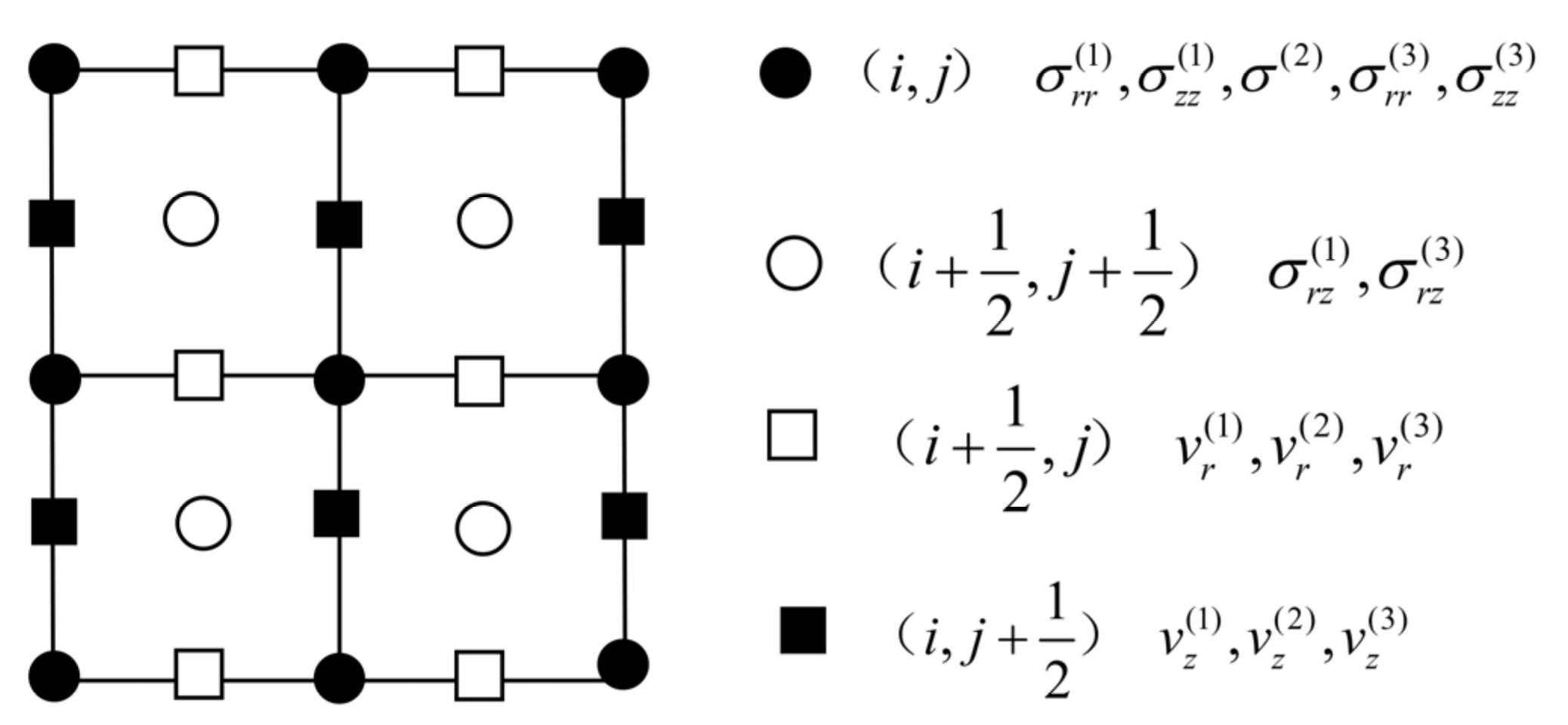
3.1. Discretization of Equations in the Carcione–Leclaire Three-Phase Theory

Figure 1 presents a schematic diagram of the acoustic logging model. A fluid-filled borehole is embedded in an unbounded three-phase porous medium (gas hydrate-bearing sediment). With a cylindrical coordinate system (r, z, $\theta$), the borehole axis lies along the central axis z of the cylinder, the monopole acoustic source is located at the center of the borehole which is placed at the origin of the coordinate system, the squares represent the receivers. As the medium is axisymmetric, all field quantities are independent of the $\theta$-coordinate. The borehole radius a is 0.1 m, ${\rho }_f$ denotes the fluid (water) density, and $v_f$ represents the fluid (water) velocity.

First, Equations (1)–(3) in a 2D axisymmetric cylindrical coordinate system can be rewritten as

$$\begin{array}{cc}\hfill & \frac{\partial }{\partial t}\left[\begin{array}{c}{\sigma }_{rr}^{\left(1\right)}\\ {\sigma }_{\theta \theta }^{\left(1\right)}\\ {\sigma }_{zz}^{\left(1\right)}\\ {\sigma }_{rz}^{\left(1\right)}\end{array}\right]\hfill \\ \hfill & =\left[\begin{array}{cccccc}{C}_1\frac{\partial }{\partial r}+\frac{D_1}{r}& D_1\frac{\partial }{\partial z}& C_{12}⟮\frac{\partial }{\partial r}+\frac{1}{r}⟯& C_{12}\frac{\partial }{\partial z}& E\frac{\partial }{\partial r}+\frac{F}{r}& F\frac{\partial }{\partial z}\\ \frac{C_1}{r}+D_1\frac{\partial }{\partial r}& D_1\frac{\partial }{\partial z}& C_{12}⟮\frac{\partial }{\partial r}+\frac{1}{r}⟯& C_{12}\frac{\partial }{\partial z}& \frac{E}{r}+F\frac{\partial }{\partial r}& F\frac{\partial }{\partial z}\\ D_1⟮\frac{\partial }{\partial r}+\frac{1}{r}⟯& C_1\frac{\partial }{\partial z}& C_{12}⟮\frac{\partial }{\partial r}+\frac{1}{r}⟯& C_{12}\frac{\partial }{\partial z}& F⟮\frac{\partial }{\partial r}+\frac{1}{r}⟯& E\frac{\partial }{\partial z}\\ {\mu }_1\frac{\partial }{\partial z}& {\mu }_1\frac{\partial }{\partial r}& 0& 0& \frac{1}{2}{\mu }_{13}\frac{\partial }{\partial z}& \frac{1}{2}{\mu }_{13}\frac{\partial }{\partial r}\end{array}\right]\left[\begin{array}{c}{v}_r^{\left(1\right)}\\ v_z^{\left(1\right)}\\ v_r^{\left(2\right)}\\ v_z^{\left(2\right)}\\ v_r^{\left(3\right)}\\ v_z^{\left(3\right)}\end{array}\right],\hfill \end{array}$$

(14)

$$\begin{array}{l}\frac{\partial {\sigma }^{(2)}}{\partial t}=C_{12}(\frac{\partial v_r^{(1)}}{\partial r}+\frac{v_r^{(1)}}{r}+\frac{\partial v_z^{(1)}}{\partial z})+K_2(\frac{\partial v_r^{(2)}}{\partial r}+\frac{v_r^{(2)}}{r}+\frac{\partial v_z^{(2)}}{\partial z})\\ \hspace{1em}\hspace{1em}\hspace{1em}+C_{23}(\frac{\partial v_r^{(3)}}{\partial r}+\frac{v_r^{(3)}}{r}+\frac{\partial v_z^{(3)}}{\partial z}),\hfill \end{array}$$

(15)

$$\begin{array}{cc}\hfill & \frac{\partial }{\partial t}\left[\begin{array}{c}{\sigma }_{rr}^{\left(3\right)}\\ {\sigma }_{\theta \theta }^{\left(3\right)}\\ {\sigma }_{zz}^{\left(3\right)}\\ {\sigma }_{rz}^{\left(3\right)}\end{array}\right]\hfill \\ \hfill & =\left[\begin{array}{cccccc}E\frac{\partial }{\partial r}+\frac{F}{r}& F\frac{\partial }{\partial z}& C_{23}⟮\frac{\partial }{\partial r}+\frac{1}{r}⟯& C_{23}\frac{\partial }{\partial z}& C_2\frac{\partial }{\partial r}+\frac{D_2}{r}& D_2\frac{\partial }{\partial z}\\ \frac{E}{r}+F\frac{\partial }{\partial r}& F\frac{\partial }{\partial z}& C_{23}⟮\frac{\partial }{\partial r}+\frac{1}{r}⟯& C_{23}\frac{\partial }{\partial z}& \frac{C_2}{r}+D_2\frac{\partial }{\partial r}& D_2\frac{\partial }{\partial z}\\ F⟮\frac{\partial }{\partial r}+\frac{1}{r}⟯& E\frac{\partial }{\partial z}& C_{23}⟮\frac{\partial }{\partial r}+\frac{1}{r}⟯& C_{23}\frac{\partial }{\partial z}& D_2⟮\frac{\partial }{\partial r}+\frac{1}{r}⟯& C_2\frac{\partial }{\partial z}\\ \frac{1}{2}{\mu }_{13}\frac{\partial }{\partial z}& \frac{1}{2}{\mu }_{13}\frac{\partial }{\partial r}& 0& 0& {\mu }_3\frac{\partial }{\partial z}& {\mu }_3\frac{\partial }{\partial r}\end{array}\right]\left[\begin{array}{c}{v}_r^{\left(1\right)}\\ v_z^{\left(1\right)}\\ v_r^{\left(2\right)}\\ v_z^{\left(2\right)}\\ v_r^{\left(3\right)}\\ v_z^{\left(3\right)}\end{array}\right],\hfill \end{array}$$

(16)

$$\begin{array}{l}{C}_1=K_1+\frac{4}{3}{\mu }_1, D_1=K_1-\frac{2}{3}{\mu }_1, C_2=K_3+\frac{4}{3}{\mu }_3, \\ D_2=K_3-\frac{2}{3}{\mu }_3, E=C_{13}+\frac{2}{3}{\mu }_{13}, F=C_{13}-\frac{1}{3}{\mu }_{13},\end{array}$$

(17)

where ${\sigma }_{rr}$, ${\sigma }_{\theta \theta }$, ${\sigma }_{zz}$ and ${\sigma }_{rz}$ are the components of the bulk stress tensor.

We define the following intermediate vector as the input for the staggered-grid finite-difference algorithm:

$W=(v_r^{(1)\prime },v_z^{(1)\prime },v_r^{(2)\prime },v_z^{(2)\prime },v_r^{(3)\prime },v_z^{(3)\prime },{\sigma }_{rr}^{(1)},{\sigma }_{\theta \theta }^{(1)},{\sigma }_{zz}^{(1)},{\sigma }_{rz}^{(1)},{\sigma }^{(2)},{\sigma }_{rr}^{(3)},{\sigma }_{\theta \theta }^{(3)},{\sigma }_{zz}^{(3)},{\sigma }_{rz}^{(3)})$. The non-stiff part in a 2D axisymmetric cylindrical coordinate system can be written as

$$\begin{array}{cc}\hfill & \frac{\partial }{\partial t}\left[\begin{array}{c}{v}_r^{\left(1\right)}\\ v_z^{\left(1\right)}\\ v_r^{\left(2\right)}\\ v_z^{\left(2\right)}\\ v_r^{\left(3\right)}\\ v_z^{\left(3\right)}\end{array}\right]=\frac{\partial }{\partial t}\left[\begin{array}{c}{v}_r^{{\left(1\right)}^{\prime }}\\ v_z^{{\left(1\right)}^{\prime }}\\ v_r^{{\left(2\right)}^{\prime }}\\ v_z^{{\left(2\right)}^{\prime }}\\ v_r^{{\left(3\right)}^{\prime }}\\ v_z^{{\left(3\right)}^{\prime }}\end{array}\right]+\left[\begin{array}{cccc}{\gamma }_{11}\left(\frac{\partial }{\partial r}+\frac{1}{r}\right)& -\frac{{\gamma }_{11}}{r}& 0& \frac{{\gamma }_{11}\partial }{\partial z}\\ 0& 0& \frac{{\gamma }_{11}\partial }{\partial z}& {\gamma }_{11}\left(\frac{\partial }{\partial r}+\frac{1}{r}\right)\\ {\gamma }_{21}\left(\frac{\partial }{\partial r}+\frac{1}{r}\right)& -\frac{{\gamma }_{21}}{r}& 0& \frac{{\gamma }_{21}\partial }{\partial z}\\ 0& 0& \frac{{\gamma }_{21}\partial }{\partial z}& {\gamma }_{21}\left(\frac{\partial }{\partial r}+\frac{1}{r}\right)\\ {\gamma }_{31}\left(\frac{\partial }{\partial r}+\frac{1}{r}\right)& -\frac{{\gamma }_{31}}{r}& 0& \frac{{\gamma }_{31}\partial }{\partial z}\\ 0& 0& \frac{{\gamma }_{31}\partial }{\partial z}& {\gamma }_{31}\left(\frac{\partial }{\partial r}+\frac{1}{r}\right)\end{array}\right.\hfill \\ \hfill & \left.\begin{array}{ccccc}\frac{{\gamma }_{12}\partial }{\partial r}& {\gamma }_{13}\left(\frac{\partial }{\partial r}+\frac{1}{r}\right)& -\frac{{\gamma }_{13}}{r}& 0& \frac{{\gamma }_{13}\partial }{\partial z}\\ \frac{{\gamma }_{12}\partial }{\partial z}& 0& 0& \frac{{\gamma }_{13}\partial }{\partial z}& {\gamma }_{13}\left(\frac{\partial }{\partial r}+\frac{1}{r}\right)\\ \frac{{\gamma }_{22}\partial }{\partial r}& {\gamma }_{23}\left(\frac{\partial }{\partial r}+\frac{1}{r}\right)& -\frac{{\gamma }_{23}}{r}& 0& \frac{{\gamma }_{23}\partial }{\partial z}\\ \frac{{\gamma }_{22}\partial }{\partial z}& 0& 0& \frac{{\gamma }_{23}\partial }{\partial z}& {\gamma }_{23}\left(\frac{\partial }{\partial r}+\frac{1}{r}\right)\\ \frac{{\gamma }_{32}\partial }{\partial r}& {\gamma }_{33}\left(\frac{\partial }{\partial r}+\frac{1}{r}\right)& -\frac{{\gamma }_{33}}{r}& 0& \frac{{\gamma }_{33}\partial }{\partial z}\\ \frac{{\gamma }_{32}\partial }{\partial z}& 0& 0& \frac{{\gamma }_{33}\partial }{\partial z}& {\gamma }_{33}\left(\frac{\partial }{\partial r}+\frac{1}{r}\right)\end{array}\right]\left[\begin{array}{c}{\sigma }_{rr}^{\left(1\right)}\\ {\sigma }_{\theta \theta }^{\left(1\right)}\\ {\sigma }_{zz}^{\left(1\right)}\\ {\sigma }_{rz}^{\left(1\right)}\\ {\sigma }^{\left(2\right)}\\ {\sigma }_{rr}^{\left(3\right)}\\ {\sigma }_{\theta \theta }^{\left(3\right)}\\ {\sigma }_{zz}^{\left(3\right)}\\ {\sigma }_{rz}^{\left(3\right)}\end{array}\right],\hfill \end{array}$$

(18)

where $v_r^{(1)}$ and $v_z^{(1)}$, $v_r^{(2)}$ and $v_z^{(2)}$, $v_r^{(3)}$ and $v_z^{(3)}$ refer to the components of the particle-velocity vector of solid grain frame, fluid and gas hydrate, respectively.

To implement a 2D finite-difference algorithm for the solutions of Equations (14)–(16) and (18), all quantities of the stress and velocity components should be discretized in staggered grids. We discretize the velocities and stresses using the staggered-grid finite-difference algorithm. The staggered-grid finite-difference form of the non-stiff part in a 2D axisymmetric cylindrical coordinate system can be expressed as (Here we only give the staggered-grid finite-difference schemes for the solid grain frame including particle velocity and stress components, which is similar to those of pore fluid and hydrate)

$$\begin{array}{l}{v}_{r(i+1/2,j)}^{(1)(n+1/2)}=v_r^{(1)}{}^{\prime }+\mathsf{\Delta }t[{\gamma }_{11}(D_r{\sigma }_{rr(i+1/2,j)}^{(1)(n)}+\frac{{{\displaystyle \sigma }}_{rr(i+1/2,j)}^{(1)(n)}-{{\displaystyle \sigma }}_{\theta \theta (i+1/2,j)}^{(1)(n)}}{r}\\ \hspace{1em}\hspace{1em}\hspace{1em}\hspace{1em}+D_z{\sigma }_{rz(i+1/2,j)}^{(1)(n)})+{\gamma }_{12}{D}_r{\sigma }_{(i,j+1/2)}^{(2)(n)}+{\gamma }_{13}(D_r{\sigma }_{rr(i+1/2,j)}^{(3)(n)}\\ \hspace{1em}\hspace{1em}\hspace{1em}\hspace{1em}+\frac{{\sigma }_{rr(i+1/2,j)}^{(3)(n)}-{\sigma }_{\theta \theta (i+1/2,j)}^{(3)(n)}}{r}+D_z{\sigma }_{rz(i+1/2,j)}^{(3)(n)})],\end{array}$$

(19)

$$\begin{array}{l}{v}_{z(i,j+1/2)}^{(1)(n+1/2)}=v_z^{(1)}{}^{\prime }+\mathsf{\Delta }t[{\gamma }_{11}(D_r{\sigma }_{rz(i,j+1/2)}^{(1)(n)}+\frac{{{\displaystyle \sigma }}_{rz(i,j+1/2)}^{(1)(n)}}{r}+D_z{\sigma }_{zz(i,j+1/2)}^{(1)(n)})\\ \hspace{1em}\hspace{1em}\hspace{1em}\hspace{1em}+{\gamma }_{12}{D}_z{\sigma }_{(i,j+1/2)}^{(2)(n)}+{\gamma }_{13}(D_r{\sigma }_{rz(i,j+1/2)}^{(3)(n)}+\frac{{\sigma }_{rz(i,j+1/2)}^{(3)(n)}}{r}\\ \hspace{1em}\hspace{1em}\hspace{1em}\hspace{1em}+D_z{\sigma }_{zz(i,j+1/2)}^{(3)(n)})],\end{array}$$

(20)

$$\begin{array}{l}{\sigma }_{rr(i,j)}^{(1)(n+1)}={\sigma }_{rr(i,j)}^{(1)(n)}+\mathsf{\Delta }t[C_1{D}_r{v}_{r(i,j)}^{(1)(n+1/2)}+D_1\frac{v_{r(i,j)}^{(1)(n+1/2)}}{r}+D_1{D}_z{v}_{z(i,j)}^{(1)(n+1/2)}\\ \hspace{1em}\hspace{1em}\hspace{1em}\hspace{1em}+C_{12}(D_r{v}_{r(i,j)}^{(2)(n+1/2)}+\frac{{{\displaystyle v}}_{r(i,j)}^{(2)(n+1/2)}}{r}+D_z{v}_{z(i,j)}^{(2)(n+1/2)})+E{D}_r{v}_{r(i,j)}^{(3)(n+1/2)}\\ \hspace{1em}\hspace{1em}\hspace{1em}\hspace{1em}+F\frac{v_{r(i,j)}^{(3)(n+1/2)}}{r}+F{D}_z{v}_{z(i,j)}^{(3)(n+1/2)}],\end{array}$$

(21)

$$\begin{array}{l}{\sigma }_{\theta \theta (i,j)}^{(1)(n+1)}={\sigma }_{\theta \theta (i,j)}^{(1)(n)}+\mathsf{\Delta }t[C_1\frac{{{\displaystyle v}}_{r(i,j)}^{(1)(n+1/2)}}{r}+D_1{D}_r{v}_{r(i,j)}^{(1)(n+1/2)}+D_1{D}_z{v}_{z(i,j)}^{(1)(n+1/2)}\\ \hspace{1em}\hspace{1em}\hspace{1em}\hspace{1em}+C_{12}(D_r{v}_{r(i,j)}^{(2)(n+1/2)}+\frac{{{\displaystyle v}}_{r(i,j)}^{(2)(n+1/2)}}{r}+D_z{v}_{z(i,j)}^{(2)(n+1/2)})+E\frac{{{\displaystyle v}}_{r(i,j)}^{(3)(n+1/2)}}{r}\\ \hspace{1em}\hspace{1em}\hspace{1em}\hspace{1em}+F{D}_r{v}_{r(i,j)}^{(3)(n+1/2)}+F{D}_z{v}_{z(i,j)}^{(3)(n+1/2)}],\end{array}$$

(22)

$$\begin{array}{l}{\sigma }_{zz(i,j)}^{(1)(n+1)}={\sigma }_{zz(i,j)}^{(1)(n)}+\mathsf{\Delta }t[C_1{D}_z{v}_{z(i,j)}^{(1)(n+1/2)}+D_1\frac{v_{r(i,j)}^{(1)(n+1/2)}}{r}+D_1{D}_r{v}_{r(i,j)}^{(1)(n+1/2)}\\ \hspace{1em}\hspace{1em}\hspace{1em}\hspace{1em}+C_{12}(D_r{v}_{r(i,j)}^{(2)(n+1/2)}+\frac{{{\displaystyle v}}_{r(i,j)}^{(2)(n+1/2)}}{r}+D_z{v}_{z(i,j)}^{(2)(n+1/2)})+E{D}_z{v}_{z(i,j)}^{(3)(n+1/2)}\\ \hspace{1em}\hspace{1em}\hspace{1em}\hspace{1em}+F\frac{v_{r(i,j)}^{(3)(n+1/2)}}{r}+F{D}_r{v}_{r(i,j)}^{(3)(n+1/2)}],\end{array}$$

(23)

$$\begin{array}{l}{\sigma }_{rz(i+1/2,j+1/2)}^{(1)(n+1)}={\sigma }_{rz(i+1/2,j+1/2)}^{(1)(n)}+\mathsf{\Delta }t[{\mu }_1(D_z{v}_{r(i+1/2,j+1/2)}^{(1)(n+1/2)}+D_r{v}_{z(i+1/2,j+1/2)}^{(1)(n+1/2)})\\ \hspace{1em}\hspace{1em}\hspace{1em}\hspace{1em}\hspace{1em}\hspace{1em}+\frac{1}{2}{\mu }_{13}(D_z{v}_{r(i+1/2,j+1/2)}^{(3)(n+1/2)}+D_r{v}_{z(i+1/2,j+1/2)}^{(3)(n+1/2)})],\end{array}$$

(24)

where n denotes the time; the subscripts i, j indicate the spatial position r, z of the field quantities, respectively; $\mathsf{\Delta }t$ is the time interval; $D_r$ and $D_z$ are discretized differential operators in $r$ and $z$ directions, respectively. In the 2D case, the distribution of the field quantities in the staggered-grid finite-difference method is shown in Figure 2.

NPML is used to eliminate the false reflection generated by artificial boundaries. In this work, the solid grain frame is taken as an example to analyze the FDTD algorithm for the first-order velocity–stress equations after using the NPML scheme. For the particle velocity components, we have

$$\begin{array}{cc}\hfill & v_{r(i+1/2,j)}^{\left(1\right)(n+1/2)}=v{{}_r^{\left(1\right)}}^{{}^{\prime }}+\mathsf{\Delta }t\left[{\gamma }_{11}\right(D_r{\sigma }_{rr(i+1/2,j)}^{\left(1\right)\left(n\right)}+P_{rrr}^{\left(1\right)\left(n\right)}+\frac{{\sigma }_{rr(i+1/2,j)}^{\left(1\right)\left(n\right)}-{\sigma }_{\theta \theta (i+1/2,j)}^{\left(1\right)\left(n\right)}}{r}\hfill \\ \hfill & \hspace{1em}\hspace{1em}\hspace{1em}\hspace{1em}+Q_{r\theta }^{\left(1\right)\left(n\right)}+D_z{\sigma }_{rz(i+1/2,j)}^{\left(1\right)\left(n\right)}+P_{rzz}^{\left(1\right)\left(n\right)})+{\gamma }_{12}(D_r{\sigma }_{(i,j+1/2)}^{\left(2\right)\left(n\right)}\hfill \\ \hfill & \hspace{1em}\hspace{1em}\hspace{1em}\hspace{1em}+P_{rrr}^{\left(2\right)\left(n\right)})+{\gamma }_{13}(D_r{\sigma }_{rrr(i+1/2,j)}^{\left(3\right)\left(n\right)}+P_{rrr}^{\left(3\right)\left(n\right)}+\frac{{\sigma }_{rr(i+1/2,j)}^{\left(3\right)\left(n\right)}-{\sigma }_{\theta \theta (i+1/2,j)}^{\left(3\right)\left(n\right)}}{r}\hfill \\ \hfill & \hspace{1em}\hspace{1em}\hspace{1em}\hspace{1em}+Q_{r\theta }^{\left(3\right)\left(n\right)}+D_z{\sigma }_{rz(i+1/2,j)}^{\left(3\right)\left(n\right)}+P_{rzz}^{\left(3\right)\left(n\right)}\left)\right],\hfill \end{array}$$

(25)

$$\begin{array}{cc}\hfill & v_{z(i,j+1/2)}^{\left(1\right)(n+1/2)}=v{{}_z^{\left(1\right)}}^{{}^{\prime }}+\mathsf{\Delta }t\left[{\gamma }_{11}\right(D_r{\sigma }_{rz(i,j+1/2)}^{\left(1\right)\left(n\right)}+P_{rzr}^{\left(1\right)\left(n\right)}+\frac{{\sigma }_{rz(i,j+1/2)}^{\left(1\right)\left(n\right)}}{r}\hfill \\ \hfill & \hspace{1em}\hspace{1em}\hspace{1em}\hspace{1em}+Q_{rz}^{\left(1\right)\left(n\right)}+D_z{\sigma }_{zz(i,j+1/2)}^{\left(1\right)\left(n\right)}+P_{zzz}^{\left(1\right)\left(n\right)})+{\gamma }_{12}(D_z{\sigma }_{(i,j+1/2)}^{\left(2\right)\left(n\right)}\hfill \\ \hfill & \hspace{1em}\hspace{1em}\hspace{1em}\hspace{1em}+P_{zzz}^{\left(2\right)\left(n\right)})+{\gamma }_{13}(D_r{\sigma }_{rz(i,j+1/2)}^{\left(3\right)\left(n\right)}+P_{rzr}^{\left(3\right)\left(n\right)}+\frac{{\sigma }_{rz(i,j+1/2)}^{\left(3\right)\left(n\right)}}{r}\hfill \\ \hfill & \hspace{1em}\hspace{1em}\hspace{1em}\hspace{1em}+Q_{rz}^{\left(3\right)\left(n\right)}+D_z{\sigma }_{zz(i,j+1/2)}^{\left(3\right)\left(n\right)}+P_{zzz}^{\left(3\right)\left(n\right)}\left)\right]\hfill \end{array}$$

(26)

where

$$P_{rrr}^n=e^{-{\mathsf{\Omega }}_r\mathsf{\Delta }t}{P}_{rrr}^{n-1}-\frac{1}{2}{\mathsf{\Omega }}_r\mathsf{\Delta }t\left[e^{-{\mathsf{\Omega }}_r\mathsf{\Delta }t}\frac{\partial {\sigma }_{rr}^{n-1}}{\partial r}+\frac{\partial {\sigma }_{rr}^n}{\partial r}\right],$$

(27)

$$P_{zzz}^n=e^{-{\mathsf{\Omega }}_z\mathsf{\Delta }t}{P}_{zzz}^{n-1}-\frac{1}{2}{\mathsf{\Omega }}_z\mathsf{\Delta }t\left[e^{-{\mathsf{\Omega }}_z\mathsf{\Delta }t}\frac{\partial {\sigma }_{zz}^{n-1}}{\partial z}+\frac{\partial {\sigma }_{zz}^n}{\partial z}\right],$$

(28)

$$P_{rzr}^n=e^{-{\mathsf{\Omega }}_r\mathsf{\Delta }t}{P}_{rzr}^{n-1}-\frac{1}{2}{\mathsf{\Omega }}_r\mathsf{\Delta }t\left[e^{-{\mathsf{\Omega }}_r\mathsf{\Delta }t}\frac{\partial {\sigma }_{rz}^{n-1}}{\partial r}+\frac{\partial {\sigma }_{rz}^n}{\partial r}\right],$$

(29)

$$P_{rzz}^n=e^{-{\mathsf{\Omega }}_{\mathrm{z}}\mathsf{\Delta }t}{P}_{rzz}^{n-1}-\frac{1}{2}{\mathsf{\Omega }}_z\mathsf{\Delta }t\left[e^{-{\mathsf{\Omega }}_z\mathsf{\Delta }t}\frac{\partial {\sigma }_{rz}^{n-1}}{\partial z}+\frac{\partial {\sigma }_{rz}^n}{\partial z}\right],$$

(30)

$$Q_{r\theta }^n=e^{-{\overline{\mathsf{\Omega }}}_r\mathsf{\Delta }t}{Q}_{r\theta }^{n-1}-\frac{1}{2}{\overline{\mathsf{\Omega }}}_r\mathsf{\Delta }t\left[e^{-{\overline{\mathsf{\Omega }}}_r\mathsf{\Delta }t}\left({\sigma }_{rr}^{n-1}-{\sigma }_{\theta \theta }^{n-1}\right)+{\sigma }_{rr}^n-{\sigma }_{\theta \theta }^n\right],$$

(31)

$$Q_{rz}^n=e^{-{\overline{\mathsf{\Omega }}}_r\mathsf{\Delta }t}{Q}_{rz}^{n-1}-\frac{1}{2}{\overline{\mathsf{\Omega }}}_r\mathsf{\Delta }t\left[e^{-{\overline{\mathsf{\Omega }}}_r\mathsf{\Delta }t}{\sigma }_{rz}^{n-1}+{\sigma }_{rz}^n\right],$$

(32)

$${\mathsf{\Omega }}_p\left(p\right)=-\frac{V_{\mathrm{pml}}\ln \alpha }{L}⟮a\frac{p}{L}+b\frac{p^2}{L^2}⟯,$$

(33)

$${\overline{\mathsf{\Omega }}}_r\left(r\right)=\frac{1}{r}{\displaystyle {\int }_0^r{\mathsf{\Omega }}_r(r\prime )dr\prime },$$

(34)

where $L$ is the width of the PML, $\alpha ={10}^{-6}$ is a predefined level of wave absorption, and the coefficients $a=0.25$ and $b=0.75$ are used.

Similar to the processing of Equations (25) and (26), Equations (21)–(24) can be discretized as

$$\begin{array}{cc}\hfill & {\sigma }_{rr(i,j)}^{\left(1\right)(n+1)}={\sigma }_{rr(i,j)}^{\left(1\right)\left(n\right)}+\mathsf{\Delta }t[C_1(D_r{v}_{r(i,j)}^{\left(1\right)(n+1/2)}+P_{rr}^{\left(1\right)(n+1/2)})+D_1(\frac{{{\displaystyle v}}_{r(i,j)}^{\left(1\right)(n+1/2)}}{r}\hfill \\ \hfill & \hspace{1em}\hspace{1em}\hspace{1em}\hspace{1em}+Q_r^{\left(1\right)(n+1/2)})+D_1(D_z{v}_{z(i,j)}^{\left(1\right)(n+1/2)}+P_{zz}^{\left(1\right)(n+1/2)})+C_{12}(D_r{v}_{r(i,j)}^{\left(2\right)(n+1/2)}\hfill \\ \hfill & \hspace{1em}\hspace{1em}\hspace{1em}\hspace{1em}+P_{rr}^{\left(2\right)(n+1/2)}+\frac{{{\displaystyle v}}_{r(i,j)}^{\left(2\right)(n+1/2)}}{r}+Q_r^{\left(2\right)(n+1/2)}+D_z{v}_{z(i,j)}^{\left(2\right)(n+1/2)}+P_{zz}^{\left(2\right)(n+1/2)})\hfill \\ \hfill & \hspace{1em}\hspace{1em}\hspace{1em}\hspace{1em}+E(D_r{v}_{r(i,j)}^{\left(3\right)(n+1/2)}+P_{rr}^{\left(3\right)(n+1/2)})+F(\frac{{{\displaystyle v}}_{r(i,j)}^{\left(3\right)(n+1/2)}}{r}+Q_r^{\left(3\right)(n+1/2)})\hfill \\ \hfill & \hspace{1em}\hspace{1em}\hspace{1em}\hspace{1em}+F(D_z{v}_{z(i,j)}^{\left(3\right)(n+1/2)}+P_{zz}^{\left(3\right)(n+1/2)})],\hfill \end{array}$$

(35)

$$\begin{array}{cc}\hfill & {\sigma }_{\theta \theta (i,j)}^{\left(1\right)(n+1)}={\sigma }_{\theta \theta (i,j)}^{\left(1\right)\left(n\right)}+\mathsf{\Delta }t[C_1(\frac{{{\displaystyle v}}_{r(i,j)}^{\left(1\right)(n+1/2)}}{r}+Q_r^{\left(1\right)(n+1/2)})+D_1(D_r{v}_{r(i,j)}^{\left(1\right)(n+1/2)}\hfill \\ \hfill & \hspace{1em}\hspace{1em}\hspace{1em}\hspace{1em}+P_{rr}^{\left(1\right)(n+1/2)})+D_1(D_z{v}_{z(i,j)}^{\left(1\right)(n+1/2)}+P_{zz}^{\left(1\right)(n+1/2)})+C_{12}(D_r{v}_{r(i,j)}^{\left(2\right)(n+1/2)}\hfill \\ \hfill & \hspace{1em}\hspace{1em}\hspace{1em}\hspace{1em}+P_{rr}^{\left(2\right)(n+1/2)}+\frac{{{\displaystyle v}}_{r(i,j)}^{\left(2\right)(n+1/2)}}{r}+Q_r^{\left(2\right)(n+1/2)}+D_z{v}_{z(i,j)}^{\left(2\right)(n+1/2)}+P_{zz}^{\left(2\right)(n+1/2)})\hfill \\ \hfill & \hspace{1em}\hspace{1em}\hspace{1em}\hspace{1em}+E(\frac{{{\displaystyle v}}_{r(i,j)}^{\left(3\right)(n+1/2)}}{r}+Q_r^{\left(3\right)(n+1/2)})+F(D_r{v}_{r(i,j)}^{\left(3\right)(n+1/2)}+P_{rr}^{\left(3\right)(n+1/2)})\hfill \\ \hfill & \hspace{1em}\hspace{1em}\hspace{1em}\hspace{1em}+F(D_z{v}_{z(i,j)}^{\left(3\right)(n+1/2)}+P_{zz}^{\left(3\right)(n+1/2)})],\hfill \end{array}$$

(36)

$$\begin{array}{cc}\hfill & {\sigma }_{zz(i,j)}^{\left(1\right)(n+1)}={\sigma }_{zz(i,j)}^{\left(1\right)\left(n\right)}+\mathsf{\Delta }t[C_1(D_z{v}_{z(i,j)}^{\left(1\right)(n+1/2)}+P_{zz}^{\left(1\right)(n+1/2)}\hfill \\ \hfill & \hspace{1em}\hspace{1em}\hspace{1em}\hspace{1em}+D_1(\frac{{{\displaystyle v}}_{r(i,j)}^{\left(1\right)(n+1/2)}}{r}+Q_r^{\left(1\right)(n+1/2)})+D_1(D_r{v}_{r(i,j)}^{\left(1\right)(n+1/2)}\hfill \\ \hfill & \hspace{1em}\hspace{1em}\hspace{1em}\hspace{1em}+P_{rr}^{\left(1\right)(n+1/2)})+C_{12}(D_r{v}_{r(i,j)}^{\left(2\right)(n+1/2)}+P_{rr}^{\left(2\right)(n+1/2)}\hfill \\ \hfill & \hspace{1em}\hspace{1em}\hspace{1em}\hspace{1em}+\frac{{{\displaystyle v}}_{r(i,j)}^{\left(2\right)(n+1/2)}}{r}+Q_r^{\left(2\right)(n+1/2)}+D_z{v}_{z(i,j)}^{\left(2\right)(n+1/2)}+P_{zz}^{\left(2\right)(n+1/2)})\hfill \\ \hfill & \hspace{1em}\hspace{1em}\hspace{1em}\hspace{1em}+E(D_z{v}_{z(i,j)}^{\left(3\right)(n+1/2)}+P_{zz}^{\left(3\right)(n+1/2)})+F(\frac{{{\displaystyle v}}_{r(i,j)}^{\left(3\right)(n+1/2)}}{r}\hfill \\ \hfill & \hspace{1em}\hspace{1em}\hspace{1em}\hspace{1em}+Q_r^{\left(3\right)(n+1/2)})+F(D_r{v}_{r(i,j)}^{\left(3\right)(n+1/2)}+P_{rr}^{\left(3\right)(n+1/2)}],\hfill \end{array}$$

(37)

$$\begin{array}{l}{\sigma }_{rz(i+1/2,j+1/2)}^{(1)(n+1)}={\sigma }_{rz(i+1/2,j+1/2)}^{(1)(n)}+\mathsf{\Delta }t[{\mu }_1(D_z{v}_{r(i+1/2,j+1/2)}^{(1)(n+1/2)}+P_{rz}^{(1)(n+1/2)}\\ \hspace{1em}\hspace{1em}\hspace{1em}\hspace{1em}+D_r{v}_{z(i+1/2,j+1/2)}^{(1)(n+1/2)}+P_{zr}^{(1)(n+1/2)})+\frac{1}{2}{\mu }_{13}(D_z{v}_{r(i+1/2,j+1/2)}^{(3)(n+1/2)}\\ \hspace{1em}\hspace{1em}\hspace{1em}\hspace{1em}+P_{rz}^{(3)(n+1/2)}+D_r{v}_{z(i+1/2,j+1/2)}^{(3)(n+1/2)}+P_{zr}^{(3)(n+1/2)})],\end{array}$$

(38)

where

$$P_{rr}^{n+1/2}=e^{-{\mathsf{\Omega }}_r\mathsf{\Delta }t}{P}_{rr}^{n-1/2}-\frac{1}{2}{\mathsf{\Omega }}_r\mathsf{\Delta }t\left[e^{-{\mathsf{\Omega }}_r\mathsf{\Delta }t}\frac{\partial v_r^{n-1/2}}{\partial r}+\frac{\partial v_r^{n+1/2}}{\partial r}\right],$$

(39)

$$P_{zz}^{n+1/2}=e^{-{\mathsf{\Omega }}_z\mathsf{\Delta }t}{P}_{zz}^{n-1/2}-\frac{1}{2}{\mathsf{\Omega }}_z\mathsf{\Delta }t\left[e^{-{\mathsf{\Omega }}_z\mathsf{\Delta }t}\frac{\partial v_z^{n-1/2}}{\partial z}+\frac{\partial v_z^{n+1/2}}{\partial z}\right],$$

(40)

$$P_{zr}^{n+1/2}=e^{-{\mathsf{\Omega }}_r\mathsf{\Delta }t}{P}_{zr}^{n-1/2}-\frac{1}{2}{\mathsf{\Omega }}_r\mathsf{\Delta }t\left[e^{-{\mathsf{\Omega }}_r\mathsf{\Delta }t}\frac{\partial v_z^{n-1/2}}{\partial r}+\frac{\partial v_z^{n+1/2}}{\partial r}\right],$$

(41)

$$P_{rz}^{n+1/2}=e^{-{\mathsf{\Omega }}_z\mathsf{\Delta }t}{P}_{rz}^{n-1/2}-\frac{1}{2}{\mathsf{\Omega }}_z\mathsf{\Delta }t\left[e^{-{\mathsf{\Omega }}_z\mathsf{\Delta }t}\frac{\partial v_r^{n-1/2}}{\partial z}+\frac{\partial v_r^{n+1/2}}{\partial z}\right],$$

(42)

$$Q_r^{n+1/2}=e^{-{\overline{\mathsf{\Omega }}}_r\mathsf{\Delta }t}{Q}_r^{n-1/2}-\frac{1}{2}{\overline{\mathsf{\Omega }}}_r\mathsf{\Delta }t\left[e^{-{\overline{\mathsf{\Omega }}}_r\mathsf{\Delta }t}{v}_z^{n-1/2}+v_z^{n+1/2}\right],$$

(43)

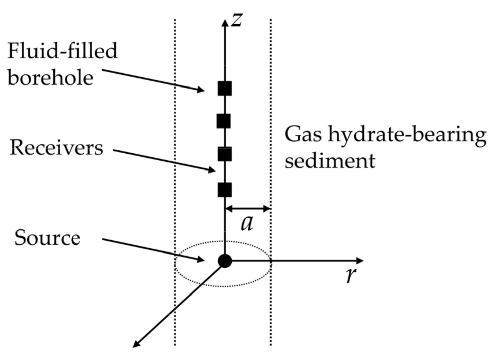
3.2. Discretization of the Equations in the Borehole and Borehole Wall

To unify the equations of acoustic wave propagation in both the outer three-phase porous medium and the inner fluid in the borehole, the limits of certain field quantities and medium parameters in the three-phase porous medium are set to obtain the equations for the fluid. In this limiting case, the stresses of the solid grain frame phase and the gas hydrate phase in the first-order velocity–stress equations of the three-phase porous medium are zero. The parameters in the Carcione–Leclaire three-phase theory change to

$$\begin{array}{l}\varphi =1,\\ K_1=K_3=0,\\ K_2=K_f,\\ C_{12}=C_{23}=C_{13}=0,\\ {\mu }_1={\mu }_{13}={\mu }_3=0,\\ {\rho }_{11}={\rho }_{12}={\rho }_{13}={\rho }_{33}={\rho }_{23}=0,\\ {\rho }_{22}={\rho }_f.\end{array}$$

(44)

In addition, according to the wave equations in fluid, it can be directly defined

$$\begin{array}{l}\exp (A_{11}\mathsf{\Delta }t)=\exp (A_{12}\mathsf{\Delta }t)=\exp (A_{13}\mathsf{\Delta }t)\\ =\exp (A_{21}\mathsf{\Delta }t)=\exp (A_{22}\mathsf{\Delta }t)=\exp (A_{23}\mathsf{\Delta }t)\\ =\exp (A_{31}\mathsf{\Delta }t)=\exp (A_{32}\mathsf{\Delta }t)=\exp (A_{33}\mathsf{\Delta }t)=0,\\ {\gamma }_{11}={\gamma }_{13}={\gamma }_{21}={\gamma }_{23}={\gamma }_{31}={\gamma }_{33}=0,\\ {\gamma }_{12}={\gamma }_{22}={\gamma }_{32}=\frac{1}{{\rho }_f}.\end{array}$$

(45)

Therefore, the equations of a three-phase porous medium degenerate into governing equations in the fluid.

4. RAI Algorithm

In the frequency wavenumber domain, the acoustic field in the borehole can be expressed as

$$\phi (r,k,\omega )=\frac{\mathrm{i}F}{{\rho }_f{\omega }^2}\left[K_0^{}\left({\alpha }_{f}r\right)\right.\left.+A(k,\omega )I_0\left({\alpha }_{f}r\right)\right],$$

(46)

where F denotes the frequency of the source; A is an undetermined coefficient, which can be regarded as the reflection coefficient of the wellbore; $K_0$ and $I_0$ are Bessel functions; r refers to the radial wave number of the fluid.

The acoustic field in a three-phase porous medium can be expressed by the displacements of solid grain frame $u_1$, pore fluid $u_2$ and gas hydrate $u_3$. The three displacements produced by a point source can be written as

$$\begin{array}{l}{u}_1=\nabla {\phi }_1+\nabla \times \nabla \times ({\eta }_1\widehat{z}),\\ u_2=\nabla {\phi }_2+\nabla \times \nabla \times ({\eta }_2\widehat{z}),\\ u_3=\nabla {\phi }_3+\nabla \times \nabla \times ({\eta }_3\widehat{z}),\end{array}$$

(47)

where ${\phi }_m$ and ${\eta }_m$ represent the displacements of compressional waves (P1, P2 and P3) and shear waves (S1 and S2), respectively. The subscripts $m$ = 1, 2, 3 refer to the solid grain frame, pore fluid and hydrate, respectively. The displacement potentials of the compressional waves in the frequency wave number domain can be expressed as

$$\begin{array}{l}{\phi }_1(r,k,\omega )=\frac{iF}{2{\rho }_f{\omega }^2}[B_1{K}_0({\alpha }_{P1}r)+C_1{K}_0({\alpha }_{P2}r)+D_1{K}_0({\alpha }_{P3}r)],\\ {\phi }_2(r,k,\omega )=\frac{iF}{2{\rho }_f{\omega }^2}[B_2{K}_0({\alpha }_{P1}r)+C_2{K}_0({\alpha }_{P2}r)+D_2{K}_0({\alpha }_{P3}r)],\\ {\phi }_3(r,k,\omega )=\frac{iF}{2{\rho }_f{\omega }^2}[B_3{K}_0({\alpha }_{P1}r)+C_3{K}_0({\alpha }_{P2}r)+D_3{K}_0({\alpha }_{P3}r)],\end{array}$$

(48)

where $B_m$, $C_m$ and $D_m$ are the undetermined amplitudes of the three compressional waves, respectively; ${\alpha }_{P1}$, ${\alpha }_{P2}$ and ${\alpha }_{P3}$ are the radial wave numbers of the three compressional waves, respectively. Moreover, in the frequency wavenumber domain, the displacement potentials of shear waves are given as

$$\begin{array}{l}{\eta }_1(r,k,\omega )=\frac{iF}{2{\rho }_f{\omega }^2}[E_1{K}_0({\alpha }_{S1}r)+F_1{K}_0({\alpha }_{S2}r)],\\ {\eta }_2(r,k,\omega )=\frac{iF}{2{\rho }_f{\omega }^2}[E_2{K}_0({\alpha }_{S1}r)+F_2{K}_0({\alpha }_{S2}r)],\\ {\eta }_3(r,k,\omega )=\frac{iF}{2{\rho }_f{\omega }^2}[E_3{K}_0({\alpha }_{S1}r)+F_3{K}_0({\alpha }_{S2}r)],\end{array}$$

(49)

where $E_m$ and $F_m$ are the undetermined amplitudes of the two shear waves, respectively; ${\alpha }_{S1}$ and ${\alpha }_{S2}$ are the radial wave numbers of the two shear waves, respectively.

In the above formulas, $A$, $B_m$, $C_m$, $D_m$, $E_m$ and $F_m$ are undetermined coefficients, which are determined by the boundary conditions of the borehole wall. Assuming that there is a relationship between the compressional wave displacement of each phase:

$${\phi }_2=l_1{\phi }_1=l_2{\phi }_3,$$

(50)

then we can obtain

$$\begin{array}{l}{B}_2=l_{11}{B}_1,C_2=l_{12}{C}_1,D_2=l_{13}{D}_1,\\ B_3=\frac{l_{11}}{l_{21}}{B}_1,C_3=\frac{l_{12}}{l_{22}}{C}_1,D_3=\frac{l_{13}}{l_{23}}{D}_1.\end{array}$$

(51)

Assuming that there is a relationship between the shear wave displacement of each phase:

$${\eta }_2=l_3{\eta }_1=l_4{\eta }_3,$$

(52)

then we can get

$$\begin{array}{l}{E}_2=l_{31}{E}_1,F_2=l_{32}{F}_1,\\ E_3=\frac{l_{31}}{l_{41}}{E}_1,F_3=\frac{l_{32}}{l_{42}}{F}_1.\end{array}$$

(53)

The boundary conditions studied in this paper are the open hole boundary conditions, which can be written as

$$\begin{array}{l}{u}_{rin}=u_{rsout}+u_{rhout}+w,\\ -{\varphi }_s{P}_{fin}={\sigma }_{rrsout},\\ -{\varphi }_h{P}_{fin}={\sigma }_{rrhout},\\ P_{fin}=P_{fout},\\ {\tau }_{rzsout}=0,\\ {\tau }_{rzhout}=0,\end{array}$$

(54)

where the subscripts in and out refer to inside and outside the borehole wall, respectively, and the subscripts s, f, and h denote solid grains, pore fluid, and hydrate, respectively. The first equation represents the continuity of fluid flow in the normal direction of the borehole wall. The second and the third equations show that the pressure of fluid in the well in the normal direction of the borehole wall is equal to the normal stress of the unit body in the gas hydrate formation outside the well in the normal direction of the borehole wall. The fourth equation represents that the pressure of the fluid in the well in the normal direction of the interface should be equal to that of the unit body in the porous formation outside the well. The fifth and sixth equations represent the continuity of shear stresses in the tangential direction of the borehole wall. $w_p$ and $w_s$ are the flowing displacement of the compressional and shear wave, which can be expressed as

$$w_P={\varphi }_f(u_2-(1-I)u_1-I{u}_3)={\varphi }_f(l_1-(1-I)-I\frac{l_1}{l_2})u_1,$$

(55)

$$w_S={\varphi }_f(u_2-(1-I)u_1-I{u}_3)={\varphi }_f(l_3-(1-I)-I\frac{l_3}{l_4})u_1,$$

(56)

where ${\varphi }_s$, ${\varphi }_f$ and ${\varphi }_h$ refer to the volume fraction of solid grains, pore fluid, and gas hydrate, respectively. $I=\frac{{\varphi }_h}{{\varphi }_h+{\varphi }_s}$, ${\varphi }_s+{\varphi }_f+{\varphi }_h=1$, ${\varphi }_f+{\varphi }_h=\varphi$. The number of boundary conditions is equal to the number of undetermined coefficients in the medium inside and outside the well. The following linear equations can be obtained by combining the displacement of the compressional and shear wave potentials and the boundary conditions of each phase

$$\left(\begin{array}{cccccc}{m}_{11}& m_{12}& m_{13}& m_{14}& m_{15}& m_{16}\\ m_{21}& m_{22}& m_{23}& m_{24}& m_{25}& m_{26}\\ m_{31}& m_{32}& m_{33}& m_{34}& m_{35}& m_{36}\\ m_{41}& m_{42}& m_{43}& m_{44}& m_{45}& m_{46}\\ m_{51}& m_{52}& m_{53}& m_{54}& m_{55}& m_{56}\\ m_{61}& m_{62}& m_{63}& m_{64}& m_{65}& m_{66}\end{array}\right)\left(\begin{array}{c}{A}_1\\ B_1\\ C_1\\ D_1\\ E_1\\ F_1\end{array}\right)=\left(\begin{array}{c}{b}_1\\ b_2\\ b_3\\ b_4\\ 0\\ 0\end{array}\right).$$

(57)

The specific solving process of each parameter in matrix M is shown in Appendix A. The reflection coefficient A in the borehole is given by

$$A=\frac{\left(\begin{array}{cccccc}{b}_1& m_{12}& m_{13}& m_{14}& m_{15}& m_{16}\\ b_2& m_{22}& m_{23}& m_{24}& m_{25}& m_{26}\\ b_{31}& m_{32}& m_{33}& m_{34}& m_{35}& m_{36}\\ b_4& m_{42}& m_{43}& m_{44}& m_{45}& m_{46}\\ 0& m_{52}& m_{53}& m_{54}& m_{55}& m_{56}\\ 0& m_{62}& m_{63}& m_{64}& m_{65}& m_{66}\end{array}\right)}{\left|M\right|}.$$

(58)

By substituting Equation (58) into Equation (46), the actual waveform received in the time domain can be obtained by the double Fourier transform.

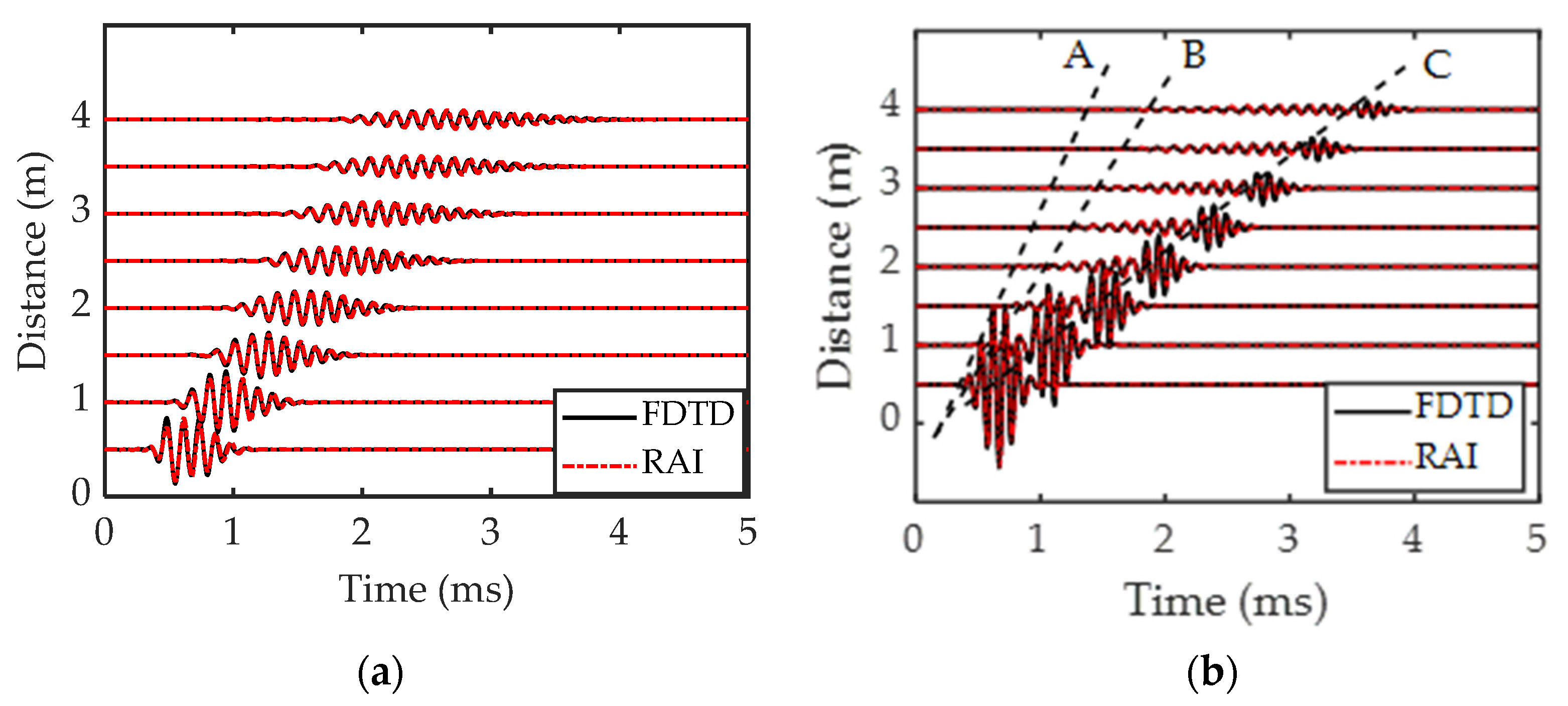
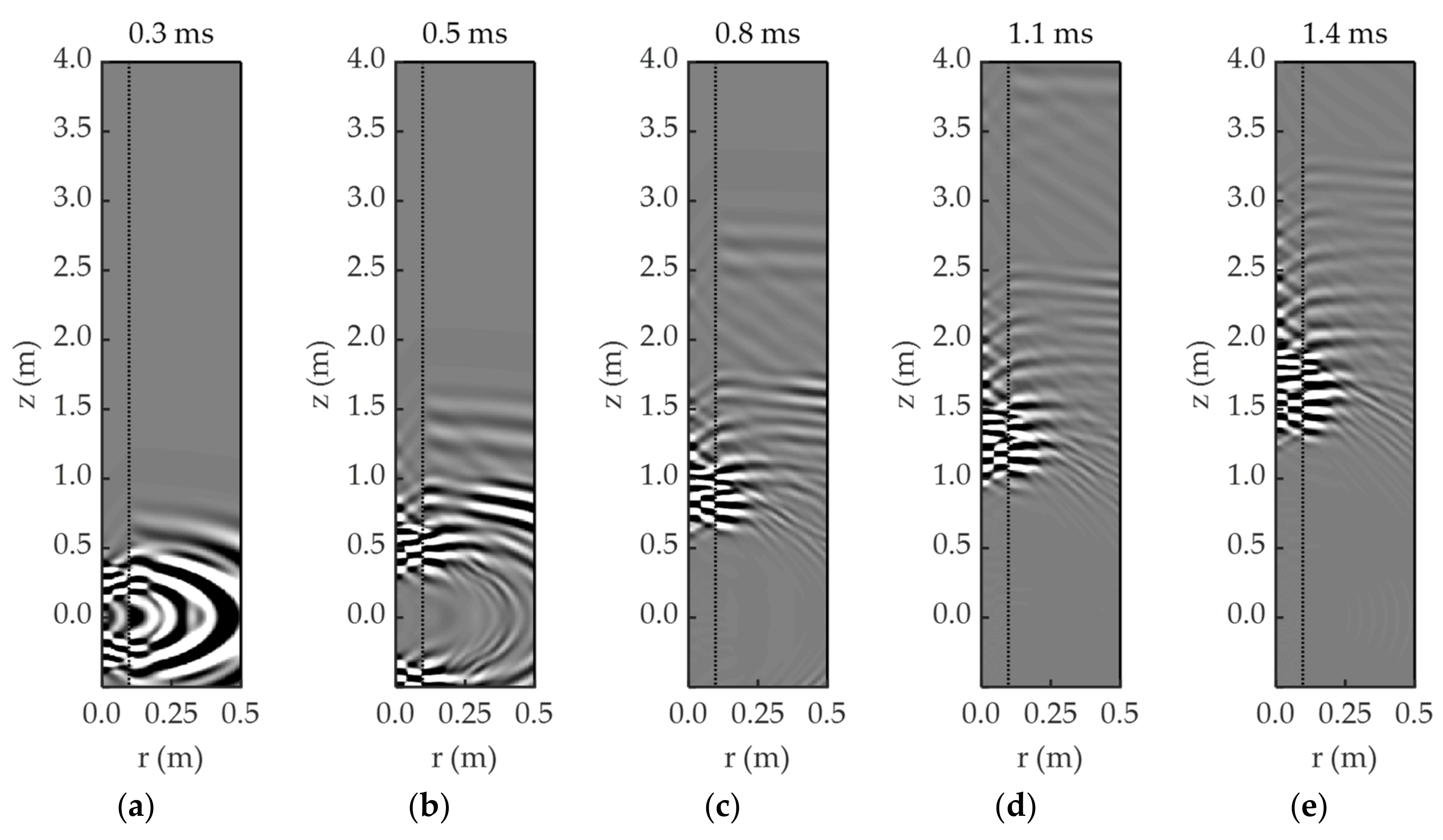
5. Numerical Modeling

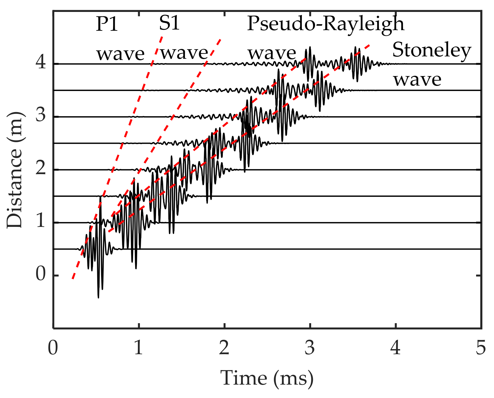
5.1. Homogeneous Three-Phase Porous Media

Figure 3 gives the simulated waveforms of the FDTD and the RAI method at different locations from z = 0.5 m to z = 4 m with different source dominant frequencies 6 kHz and 10 kHz in the gas hydrate formation. The physical parameters of the gas hydrate-bearing sediment are given in

Table 1. Physical parameters of the model.

Parameter	Value
Grain density (kg/m3)	2650
Fluid density (kg/m3)	1000
Gas hydrate density (kg/m3)	900
Grain bulk modulus (GPa)	38.7
Fluid bulk modulus (GPa)	2.25
Gas hydrate bulk modulus (GPa)	8.85
Gas hydrate shear modulus (GPa)	3.32
Grain frame permeability ${\kappa }_{so}$ (m2)	1.07 × 10−13
Gas hydrate frame permeability ${\kappa }_{ho}$ (m2)	5 × 10−4

. The acoustic source pulse width T_c = 0.5 ms is employed in our simulation. The radius of the borehole is 0.1 m. In our FDTD scheme, the time step is $2\times {10}^{-4}$ ms and the space steps in the r and z directions are both chosen as $5\times {10}^{-4}$ m. The radial length of the model is 0.5 m, while the axial length is 4.0 m. The width L of the NPML region is 0.5 m. The source pulse function s(t) used in this paper is expressed as

$$s(t)=\left\{\begin{array}{c}\frac{1}{2}\left[1+\cos \frac{2\pi }{T_c}⟮t-\frac{T_c}{2}⟯\right]\cos 2\pi f_0⟮t-\frac{T_c}{2}⟯, 0\le \mathrm{t}\le T_c\\ 0 , t>T_c\hfill \end{array}\right.,$$

(59)

where $f_0$ refers to the center frequency of the source, and t denotes the time. Figure 3b shows that there are three different wave groups of the waveforms: the first kind of compressional (P1) wave (A), the first kind of shear (S1) wave (B), and the Stoneley wave (C). The amplitude of the P1 wave is small, while the S1 wave and Stoneley wave are more evident. As depicted in Figure 3, the FDTD algorithm simulations (black solid lines) agree well with the RAI solutions (red dash-dot lines) at different locations from z = 0.5 m to z = 4 m. Because of the discrete Fourier transform of the RAI method and the discrete FDTD grids, there are small differences in the amplitudes of the waveforms of the two methods [41].

As an example of using the finite-difference scheme proposed above, we simulate the acoustic field in a wellbore surrounded by a three-phase porous medium. The wave field distribution at instants of 0.3, 0.5, 0.8, 1.1, and 1.4 ms is displayed in Figure 4. The black dotted line represents the borehole wall. To identify different wave groups in the wave field, a domain frequency $f_0$= 20 kHz and a shorter pulse width $T_c$ = 0.2 ms are employed in our simulation. The time and space steps are consistent with those in Figure 3. Figure 4a–e shows that there is no evident wave reflection from the outer boundaries, which indicates that the wave field is well absorbed in the NPML. In Figure 4a, we can observe the fastest pulse in the formation is the P1 wave and then the S1 wave. When the direct wave propagates to the borehole wall, part of the energy propagates outward, forming the refraction waves. Because there is no friction between the solid grain and the gas hydrate and the viscosity of the pore fluid is $1.8\times {10}^{-3}$ Pa·s, four waves exist in the gas hydrate formation: two compressional waves (P1 and P2) and two shear waves (S1 and S2) [44]. As indicated in Figure 4, the energy of the Stoneley wave is mainly concentrated near the interface of the borehole wall, which is the same as that in a two-phase porous medium [37]. With the increase of time, the amplitude of the Stoneley wave attenuates. Furthermore, the compressional head wave in the borehole can also be observed.

Figure 5 gives the simulated waveforms with a dominant frequency $f_0$ = 20 kHz and a pulse width $T_c$ = 0.2 ms, the frequency range is 10 kHz–30 kHz. Figure 5 shows that there exist four different wave groups of the waveforms: the first kind of compressional (P1) wave, the first kind of shear (S1) wave, the pseudo-Rayleigh wave, and the Stoneley wave. The amplitudes of the pseudo-Rayleigh wave and Stoneley wave are much larger than those of the P1 and S1 waves. Because of the different physical characteristics of each component, there is a certain difference among the propagation velocities of the four waves. The pseudo-Rayleigh wave is a kind of interface wave, and its low-frequency cutoff velocity is usually the velocity of the S1 wave, and the velocity difference between the pseudo-Rayleigh wave and S1 wave is small. As can be observed in Figure 5, with the increase of the distance between the receiver and the source, the amplitudes of the four modes become smaller. The relative motion between the viscous fluid and the solid phase of the three-phase porous media causes viscous dissipation and dissipation of wave energy, the four waves are attenuated in the process of propagation. Moreover, P2 and S2 waves are not observed in the wave field because of their small amplitudes and large attenuation along the axis of the well.

The estimation of gas hydrate saturation in a hydrate reservoir is a key index in hydrate exploration. The P1-wave velocity and attenuation were used to evaluate hydrate saturation in previous studies [45,46]. However, there is no research on the analysis of the Stoneley wave in gas hydrate reservoirs. The Stoneley wave is usually used to evaluate the permeability of fluid-saturated porous media. Here, we further investigate the waveforms in the borehole with different gas hydrate saturations (Figure 6) with the domain frequency $f_0$ = 10 kHz. Gas hydrate saturations of 0.4, 0.5, and 0.6 are considered. From Figure 6, it can be observed that the variation of the Stoneley wave amplitude with gas hydrate saturation is larger than those of the P1 wave and the S1 wave. Further, with the increase of hydrate saturation, the velocity of the Stoneley wave is almost unchanged, while the amplitude of the Stoneley wave decreases significantly. Under the condition of the same gas hydrate saturation, with the increase of the source-receiver distance, the Stoneley wave attenuates, and its amplitude decreases. Further, the attenuation coefficient of the Stoneley wave is calculated at different gas hydrate saturations. The amplitude of Stoneley wave A [47] can be expressed as

$$A={\left(\frac{{\displaystyle \sum _{i=1}^M{(W_i)}^2}}{M}\right)}^{\frac{1}{2}},$$

(60)

where M is sampling numbers; $W_i$ denotes the amplitude of the sampling point i. The attenuation coefficient of the Stoneley wave [47] is given by

$${\alpha }_{ST}=\frac{2\lg (A_n/A_m)}{(m-n)d_s},$$

(61)

where $A_n$ and $A_m$ represent the amplitudes of the received waveforms of the n-th and the m-th receivers, respectively; $d_s$ is the receiver spacing. After calculation, we find that when values of the hydrate saturation are 0.4, 0.5, and 0.6, the attenuation coefficients of the Stoneley wave are 0.35, 0.52, and 0.87, respectively. The results indicate that the attenuation coefficient of the Stoneley wave increases with the increase of gas hydrate saturation. Thus, we can use the attenuation of the Stoneley wave to estimate the gas hydrate saturation of the reservoir.

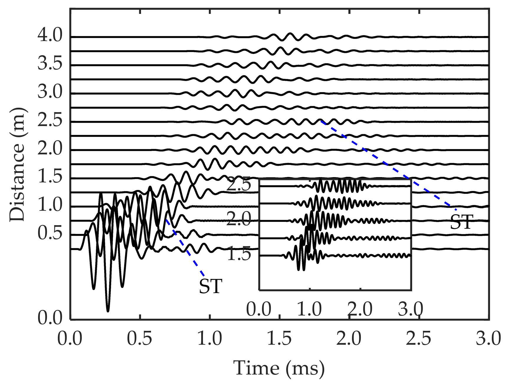
5.2. Horizontally Stratified Three-Phase Porous Medium

Presented in Figure 7 is a schematic diagram of a horizontally stratified medium across a borehole on the r–z plan. The borehole is filled with water. As shown in Figure 7, there are three layers in the formation around the borehole, the layer between 1.0 m and 2.5 m is the gas hydrate-bearing sediment, the other two layers are elastic media. The parameters of the gas hydrate formation are consistent with those shown in Table 1, while the parameters in the other two elastic layers are the same as those of the solid grains in the hydrate formation. Fluid–hydrate, solid–hydrate, and fluid–solid interfaces exist in this model. We use the FDTD algorithm combined with the parameter averaging technique to simulate the wave propagation in the borehole. Shown in Figure 8 is the wave-field distribution at instants of 0.5, 1.0, 1.5, and 2.0 ms. The interfaces are marked with two blue lines. In our simulation, the source has a center frequency and a pulse width of $f_0$ = 10 kHz and a pulse width $T_c$ = 0.5 ms, the frequency range is 6 kHz–14 kHz. The time and space steps are consistent with those in the homogeneous three-phase medium. In the figure, no evident wave reflection is observed from the outer boundaries, indicating that the wave-field is well absorbed in the NPMLs. As indicated in Figure 8, the energy of the Stoneley wave is reflected at the interface. Figure 9 displays the waveforms at different locations along the borehole. In Figure 9, the two blue lines indicate the reflected Stoneley waves at the two interfaces. It can be seen that the amplitude of the Stoneley wave from the upper interface is smaller than that from the bottom interface. This is because most of the wave energy is attenuated in the interlayer and transmitted from the interface. Further, because the layers of 0 m–1.0 m and 2.5 m–4.0 m are two identical elastic media while the interlayer of 1.0 m–2.5 m is a gas hydrate-bearing sediment, it can be seen from the waveforms that the velocity of the Stoneley wave is the same when the distance between the receiver and the source is within 1 m and between 2.5 m and 4 m. Besides, when the distance between the receiver and the source is between 1.0 m and 2.5 m, the velocity of the Stoneley wave is obviously smaller than the other two cases.

6. Conclusions

To extract hydrate information from acoustic data, we have developed both an RAI and a velocity–stress FDTD algorithm with a nonsplitting perfect matched layer to simulate acoustic wave propagation in the borehole surrounded by a gas hydrate-bearing sediment. The proposed FDTD algorithm can also be applied for simulations of acoustic logs in a heterogeneous three-phase porous medium. Clearly reflected Stoneley waves generated from the upper and lower interfaces of the different media can be observed in the waveforms. The above work can enrich our understanding of wave propagation in the borehole surrounded by a gas hydrate formation and provide a theoretical foundation for the exploration and development of hydrate.

References

1. Ruppel, C. Tapping methane hydrates for unconventional natural gas. Elements 2007, 3, 193–199. [Google Scholar] [CrossRef]
2. Boswell, R. Is gas hydrate energy within reach. Science 2009, 325, 957–958. [Google Scholar] [CrossRef] [PubMed]
3. Chong, Z.R.; Yang, S.H.B.; Babu, P.; Linga, P.; Li, X.S. Review of natural gas hydrates as an energy resource: Prospects and challenges. Appl. Energy 2016, 162, 1633–1652. [Google Scholar] [CrossRef]
4. Sadeq, D.; Alef, K.; Iglauer, S.; Lebedev, M.; Barifcani, A. Compressional wave velocity of hydrate-bearing Bernheimer sediments with varying pore fillings. Int. J. Hydrogen Energy 2018, 43, 23193–23200. [Google Scholar] [CrossRef]
5. Liu, T.; Liu, X.; Zhu, T. Joint analysis of P-wave velocity and resistivity for morphology identification and quantification of gas hydrate. Mar. Pet. Geol. 2019, 112, 104036–104048. [Google Scholar] [CrossRef]
6. Yuan, Q.M.; Kong, L.; Xu, R.; Zhao, Y.P. A state-dependent constitutive model for gas hydrate-bearing sediments considering cementing effect. J. Mar. Sci. Eng. 2020, 8, 621. [Google Scholar] [CrossRef]
7. Mahabadi, N.; Dai, S.; Seol, Y.; Jang, J. Impact of hydrate saturation on water permeability in hydrate-bearing sediments. J. Pet. Sci. Eng. 2019, 174, 696–703. [Google Scholar] [CrossRef]
8. Lee, M.W.; Waite, W.F. Estimating pore-space gas hydrate saturations from well log acoustic data. Geochem. Geophys. Geosyst. 2008, 9, Q07008. [Google Scholar] [CrossRef] [Green Version]
9. Ding, J.P.; Cheng, Y.F.; Deng, F.C.; Yang, C.L.; Sun, H.; Li, Q.C.; Song, B.G. Experimental study on dynamic acoustic characteristics of natural gas hydrate sediments at different depths. Int. J. Hydrogen Energy 2020, 45, 26877–26889. [Google Scholar] [CrossRef]
10. Leclaire, P.; Cohen-Tenooudji, F.; Puente, J. Extension of Biot’s theory of wave propagation to frozen porous media. J. Acoust. Soc. Am. 1994, 96, 3753–3768. [Google Scholar] [CrossRef] [Green Version]
11. Carcione, J.M.; Seriani, G. Wave simulation in frozen porous media. J. Comput. Phys. 2001, 170, 676–695. [Google Scholar] [CrossRef] [Green Version]
12. Malinverno, A.; Kastner, M.; Torres, M.E.; Wortmann, U.G. Gas hydrate occurrence from pore fluid chlorinity and downhole logs in a transect across the northern Cascadia margin (Integrated Ocean Drilling Program Expedition 311). J. Geophys. Res. Solid Earth 2008, 113, B08103. [Google Scholar] [CrossRef]
13. Liu, L.; Jiang, G.S.; Ning, F.L.; Yu, Y.B.; Zhang, L.; Tu, Y.Z. Well logging in gas hydrate-bearing sediment: A review. Adv. Mater. Res. 2012, 524–527, 1660–1670. [Google Scholar] [CrossRef]
14. Carcione, J.M.; Gei, D. Gas-hydrate concentration estimated from P- and S-wave velocities at the Mallik 2L-38 research well, Mackenzie Delta. J. Appl. Geophys. 2014, 56, 73–78. [Google Scholar] [CrossRef]
15. Yan, C.L.; Cheng, Y.F.; Li, M.L.; Han, Z.Y.; Zhang, H.W.; Li, Q.C.; Teng, F.; Ding, J.P. Mechanical experiments and constitutive model of natural gas hydrate reservoirs. Int. J. Hydrogen Energy 2017, 42, 19810–19818. [Google Scholar] [CrossRef]
16. Bei, K.Q.; Xu, T.F.; Shang, S.H.; Wei, Z.L.; Yuan, Y.L.; Tian, H.L. Numerical modeling of gas migration and hydrate formation in heterogeneousmarine sediments. J. Mar. Sci. Eng. 2019, 7, 348. [Google Scholar] [CrossRef] [Green Version]
17. Nair, V.C.; Prasad, S.K.; Sangwai, J.S. Characterization and Rheology of Krishna-Godavari basin Sediments. Mar. Pet. Geol. 2019, 110, 275–286. [Google Scholar] [CrossRef]
18. Kumari, A.; Balomajumder, C.; Arora, A.; Dixit, G.; Gomari, S.R. Physio-Chemical and Mineralogical Characteristics of Gas Hydrate-Bearing Sediments of the Kerala-Konkan, Krishna-Godavari, and Mahanadi Basins. J. Mar. Sci. Eng. 2021, 9, 808. [Google Scholar] [CrossRef]
19. Rosenbaum, J.H. Synthetic microseismograms: Logging in porous formations. Geophysics 1974, 39, 14–32. [Google Scholar] [CrossRef]
20. Biot, M.A. General theory of three-dimensional consolidation. J. Appl. Phys. 1941, 12, 155–164. [Google Scholar] [CrossRef]
21. Biot, M.A. Theory of propagation of elastic waves in a fluid-saturated porous solid, I-low frequency range. J. Acoust. Soc. Am. 1956, 28, 168–178. [Google Scholar] [CrossRef]
22. Biot, M.A. Theory of propagation of elastic waves in a fluid-saturated porous solid, II-higher-frequency range. J. Acoust. Soc. Am. 1956, 28, 179–191. [Google Scholar] [CrossRef]
23. Biot, M.A.; Willis, D.G. The elastic coefficients of the theory of consolidation. J. Appl. Mech. 1957, 24, 594–601. [Google Scholar] [CrossRef]
24. Biot, M.A. Mechanics of deformation and acoustic propagation in porous media. J. Appl. Phys. 1962, 33, 1482–1498. [Google Scholar] [CrossRef]
25. Biot, M.A. Generalized theory of acoustic propagation in porous dissipative media. J. Acoust. Soc. Am. 1962, 34, 1254–1264. [Google Scholar] [CrossRef]
26. Wang, K.X.; Dong, Q.D. Theoretical analysis and calculation of sound field in an oil well surrounded by a permeable formation. Acta Pet. Sin. 1986, 7, 59–69. [Google Scholar] [CrossRef]
27. Wang, K.X.; White, J.E.; Wu, X.Y. P-wave coupling to hole in Biot solid. Acta Geophys. Sin. 1996, 39, 103–113. [Google Scholar]
28. Schmitt, D.P. Effects of radial layering when logging in saturated porous formations. J. Acoust. Soc. Am. 1988, 84, 2200–2214. [Google Scholar] [CrossRef]
29. He, X. Mode Waves in a Fluid-Filled Borehole Embedded in a Porous Formation. Master’s Thesis, Harbin Institute of Technology, Harbin, China, 2006. [Google Scholar]
30. Xu, N. Simulation of Acoustic Fields and Inversion of Permeability from Attenuation of Stoneley Waves in Permeable Borehole. Master’s Thesis, Jilin University, Jilin, China, 2011. [Google Scholar]
31. Wang, S.L. Study on Permeability Inversion by Using Dipole Acoustic Logging Data. Master’s Thesis, School of Geosciences China University of Petroleum (EastChina), Qingdao, China, 2011. [Google Scholar]
32. Xu, X.K.; Chen, X.L.; Fan, Y.R.; Li, X.; Liu, M.J.; Hu, H.C. Influence factors of Stoneley wave and permeability inversion of formation. J. China Univ. Pet. 2012, 36, 97–104. [Google Scholar] [CrossRef]
33. Liu, X.E.; Sun, X.F. On inversion method of the flexural wave permeability. Well Logging Technol. 2014, 38, 674–677. [Google Scholar]
34. Xu, X.K.; Fan, Y.R.; Zhai, Y.; Wang, S.L.; Liu, M.J. Influence factors analysis of flexural wave permeability inversion in low porosity and low permeability reservior. Well Logging Technol. 2017, 41, 400–404. [Google Scholar]
35. Zhang, M.Y. Study on the Influence of Viscous Pore Fluid Stress on Body Waves in Porous Media and Borehole Waves. Master’s Thesis, Harbin Institute of Technology, Harbin, China, 2020. [Google Scholar]
36. Kristek, J.; Moczo, P.; Chaljub, E.; Kristekova, M. An orthorhombic representation of a heterogeneous medium for the finite-difference modelling of seismic wave propagation. Geophys. J. Int. 2017, 208, 1250–1264. [Google Scholar] [CrossRef]
37. Guan, W.; Hu, H.; He, X. Finite-difference modeling of the monopole acoustic logs in a horizontally stratified porous formation. J. Acoust. Soc. Am. 2009, 125, 1942–1950. [Google Scholar] [CrossRef] [PubMed]
38. Guan, W.; Hu, H. The parameter averaging technique in finite-difference modeling of elastic waves in combined structures with solid, fluid and porous subregions. Commun. Comput. Phys. 2011, 10, 695–715. [Google Scholar] [CrossRef]
39. Wang, T.; Tang, X.M. Finite-difference modeling of elastic wave propagation: A nonsplitting perfectly matched layer approach. Geophysics 2003, 68, 1749–1755. [Google Scholar] [CrossRef]
40. Yan, S.G.; Xie, F.L.; Gong, D.; Zhang, C.G.; Zhang, B.X. Borehole acoustic fields in porous formation with tilted thin fracture. Chin. J. Geophys. 2015, 58, 307–313. [Google Scholar] [CrossRef]
41. Ou, W.; Wang, Z. Simulation of Stoneley wave reflection from porous formation in borehole using FDTD method. Geophys. J. Int. 2019, 217, 2081–2096. [Google Scholar] [CrossRef]
42. Carcione, J.M.; Quiroga-Goode, G. Some aspects of the physics and numerical modeling of Biot compressional waves. J. Comput. Acoust. 1995, 3, 261–272. [Google Scholar] [CrossRef]
43. Zhao, H.; Wang, X.; Chen, H. A method of solving the stiffness problem in Biot’s poroelastic equations using a staggered high-order finite-difference. Chin. Phys. 2006, 15, 2819–2827. [Google Scholar] [CrossRef]
44. Lin, L.; Zhang, X.; Wang, X. Theoretical analysis and numerical simulation of acoustic waves in gas hydrate-bearing sediments. Chin. Phys. B 2021, 30, 024301. [Google Scholar] [CrossRef]
45. Zhang, R.; Li, H.; Wen, P.; Zhang, B. The velocity dispersion and attenuation of marine hydrate-bearing sediments. Chin. J. Geophys. 2016, 59, 539–550. [Google Scholar]
46. Lin, L.; Zhang, X.; Wang, X. Wave propagation characteristics in gas hydrate-bearing sediments and estimation of hydrate saturation. Energies 2021, 14, 804. [Google Scholar] [CrossRef]
47. Mu, Y.; Zhang, L.; Luo, S.; Wu, Y.; Cui, W.; Miao, X.; Mu, H. Permeability evaluation of carbonate reservoirs through Stoneley wave energies analysis. Well Logging Technol. 2019, 43, 386–390. [Google Scholar]
Figure 1. Schematic diagram of the acoustic logging model. The fluid-filled borehole is embedded in a three-phase porous medium. The borehole radius a is 0.1 m. The monopole acoustic source and the receivers are along the borehole axis, and the source is located at the origin of the cylindrical coordinate system.
Jmse 10 00235 g001
Figure 2. Distribution of the field components in the staggered-grid finite-difference algorithm in cylindrical coordinates.
Jmse 10 00235 g002
Figure 3. Comparisons between the FDTD and the RAI methods of the simulated waveforms of the acoustic logs in a gas hydrate formation. The center frequency of the source is (a) 6 kHz, (b) 10 kHz.
Jmse 10 00235 g003
Figure 4. Simulation of the wave field distribution at five instants of (a) 0.3 ms, (b) 0.5 ms, (c) 0.8 ms, (d) 1.1 ms, and (e) 1.4 ms of the acoustic logs in the gas hydrate-bearing sediment. The source is located at the origin. The dominant frequency of the source is 20 kHz.
Jmse 10 00235 g004
Figure 5. Simulated waveforms of the acoustic logs in a gas hydrate formation. The center frequency of the source is 20 kHz.
Jmse 10 00235 g005
Figure 6. Simulated waveforms of the acoustic logs in a gas hydrate formation of different gas hydrate saturations. Gas hydrate saturation of 0.4, 0.5, and 0.6 are considered. The center frequency of the source is 10 kHz.
Jmse 10 00235 g006
Figure 7. Schematic diagram of a horizontal stratified three-phase porous medium (gas hydrate-bearing sediment) across a borehole on the r-z plan.
Jmse 10 00235 g007
Figure 8. Simulation of the wave-eld distribution at four instants of (a) 0.5 ms, (b) 1.0 ms, (c) 1.5 ms, and (d) 2.0 ms of the acoustic logs in the horizontally stratified three-phase porous medium. The source is located at 0.5 m. The dominant frequency of the source is 10 kHz. The layer between 1.5 m and 3.0 m is the gas hydrate-bearing sediment. The other two layers are two elastic formations.
Jmse 10 00235 g008
Figure 9. Waveforms at different locations along the borehole of the acoustic logs in a horizontally stratified three-phase porous medium (gas hydrate-bearing sediment). The longitudinal axis is the distance from the receiver to the source.
Jmse 10 00235 g009