
Modelling the Effect of ‘Roller Dynamics’ on Storm Erosion: Sylt, North Sea


Abstract
:1. Introduction
2. Study Area
2.1. Background
2.2. Field Data
3. Methodology
3.1. Model Setup
3.1.1. Modelling Tools
- (a)
- Delft3D (D3D)
- (b)
- XBeach (XB)
3.1.2. Roller Model
- (a)
- Beta (β)
- (b)
- Gamdis
- (c)
- F_lam
3.1.3. Model Domains and Boundary Forcing
3.1.4. Simulations
3.2. Analysis
- (a)
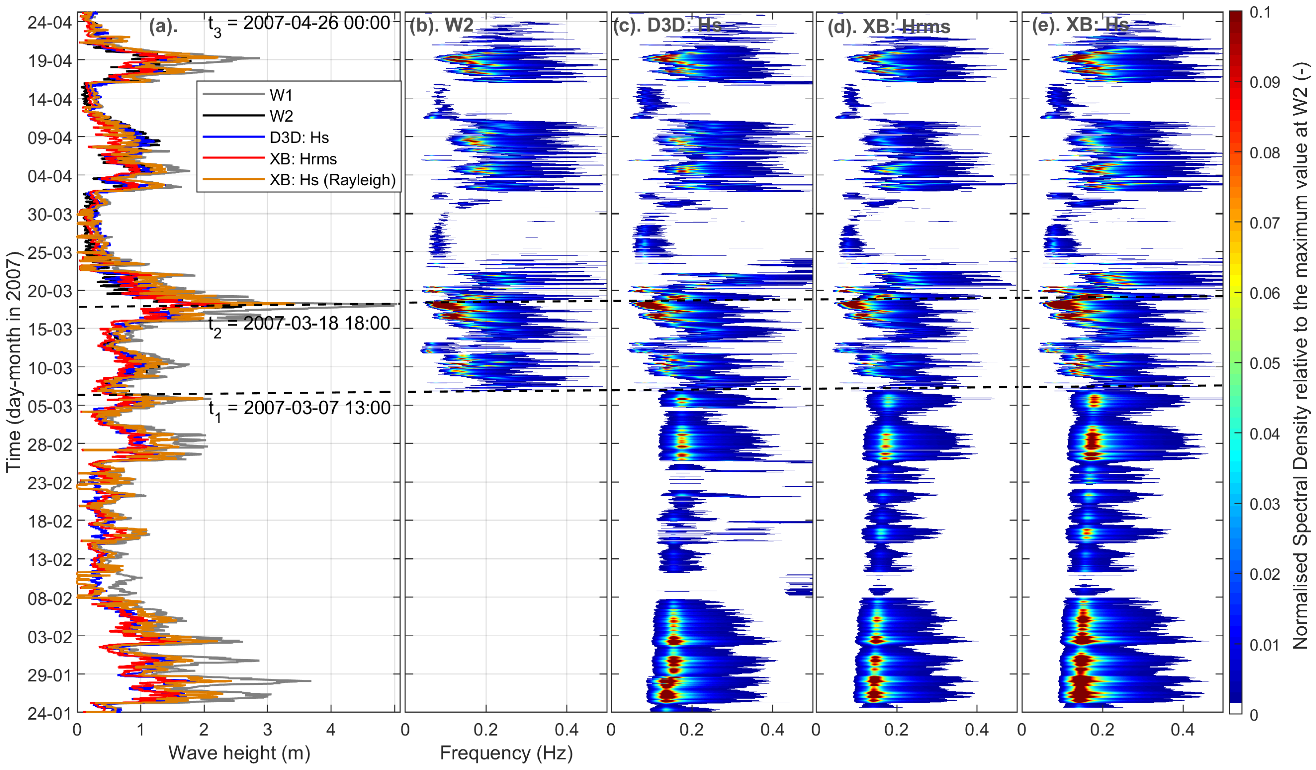
- Wave spectral density
- (b)
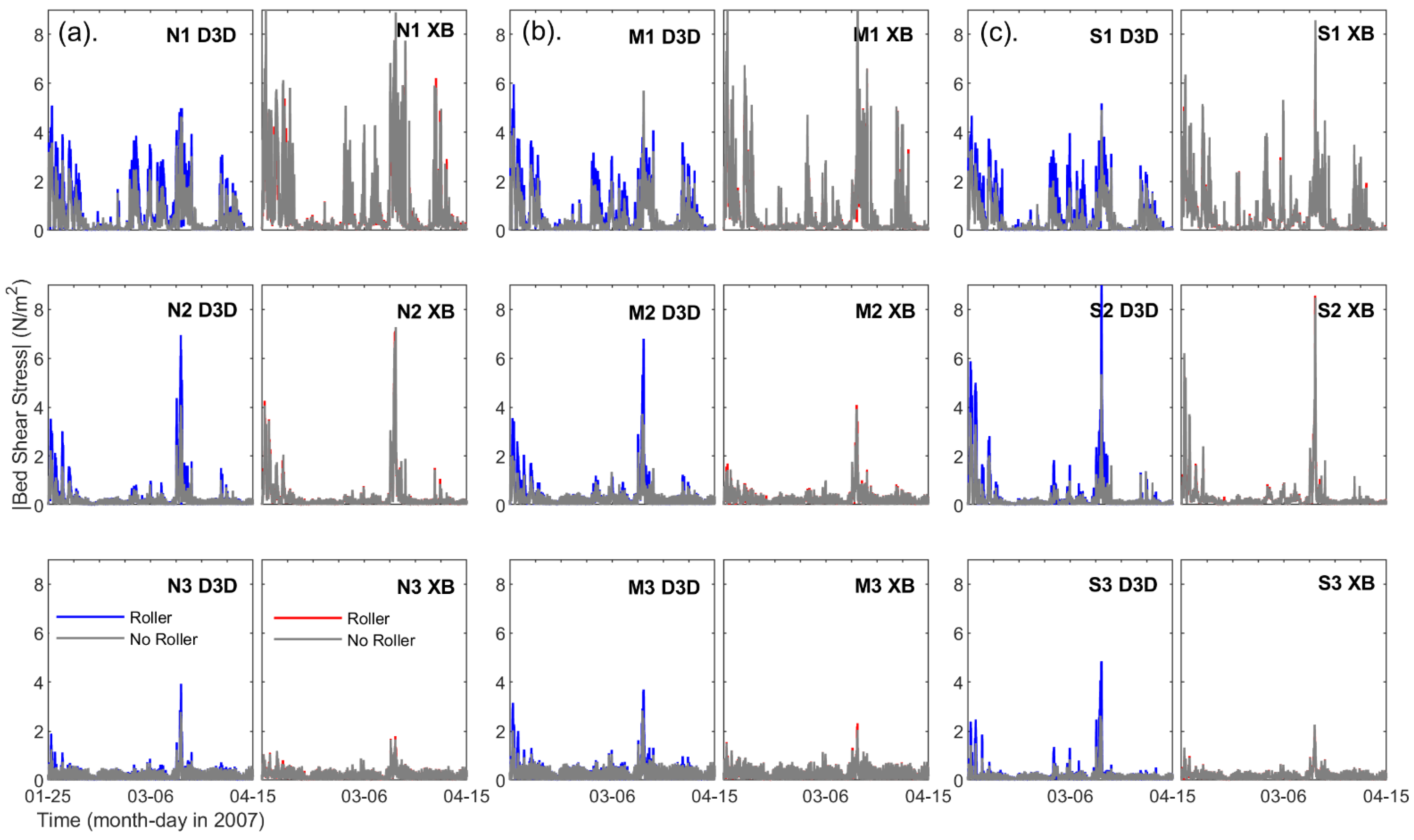
- Effective bed shear stress
- (c)
- Statistical parameters
4. Results
4.1. Model Skill
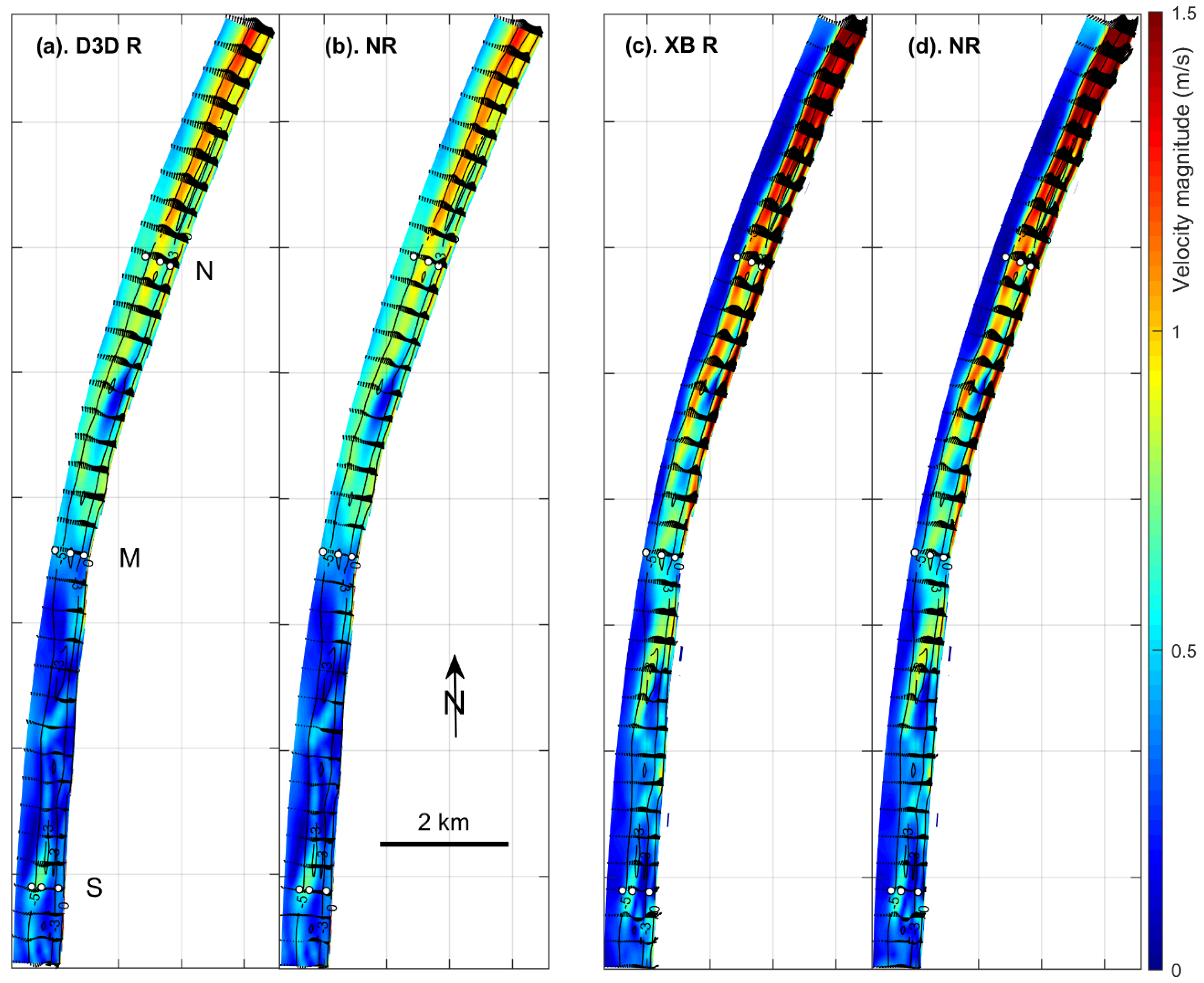
4.2. Hydrodynamics
4.3. Storm Erosion
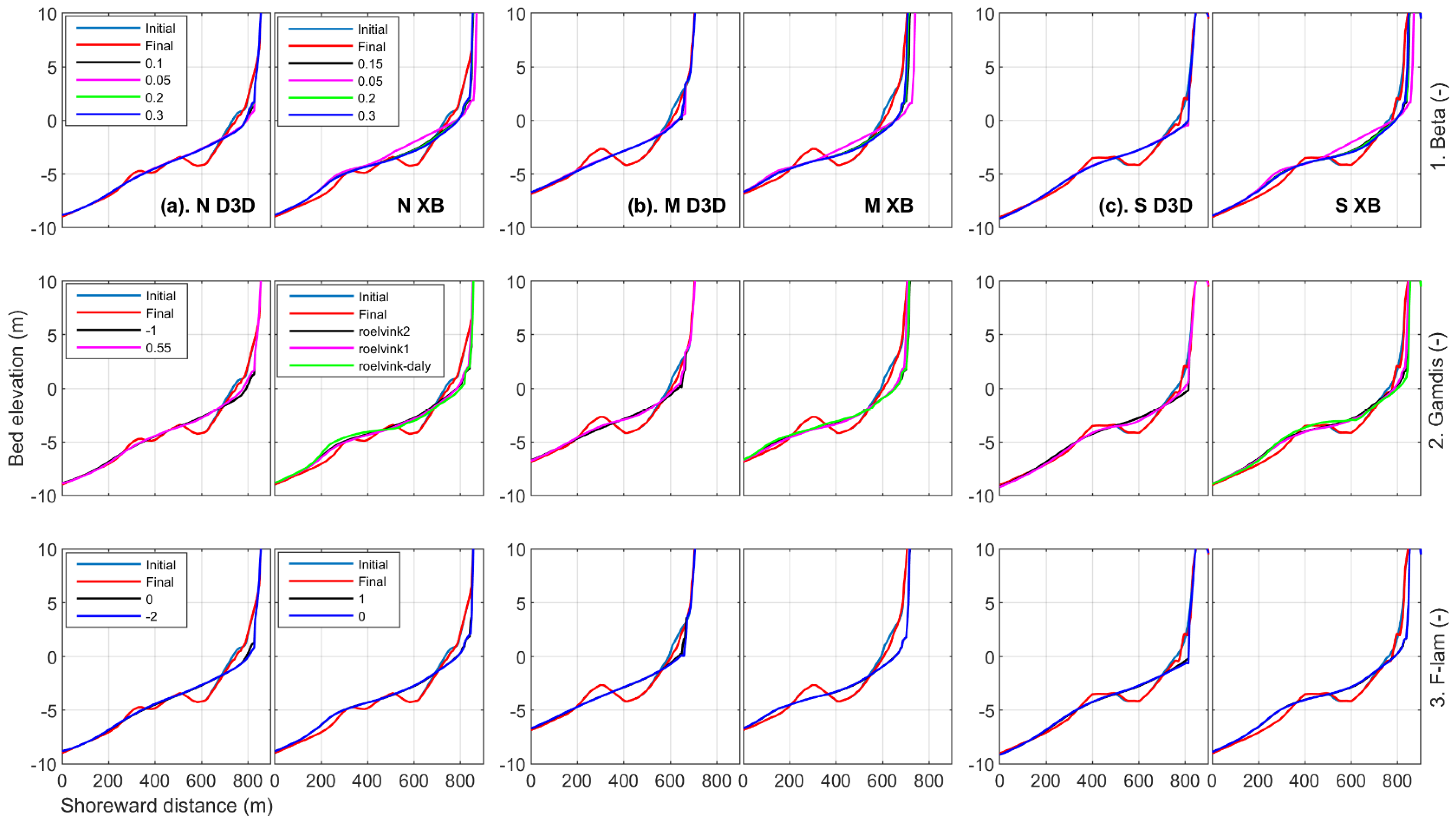
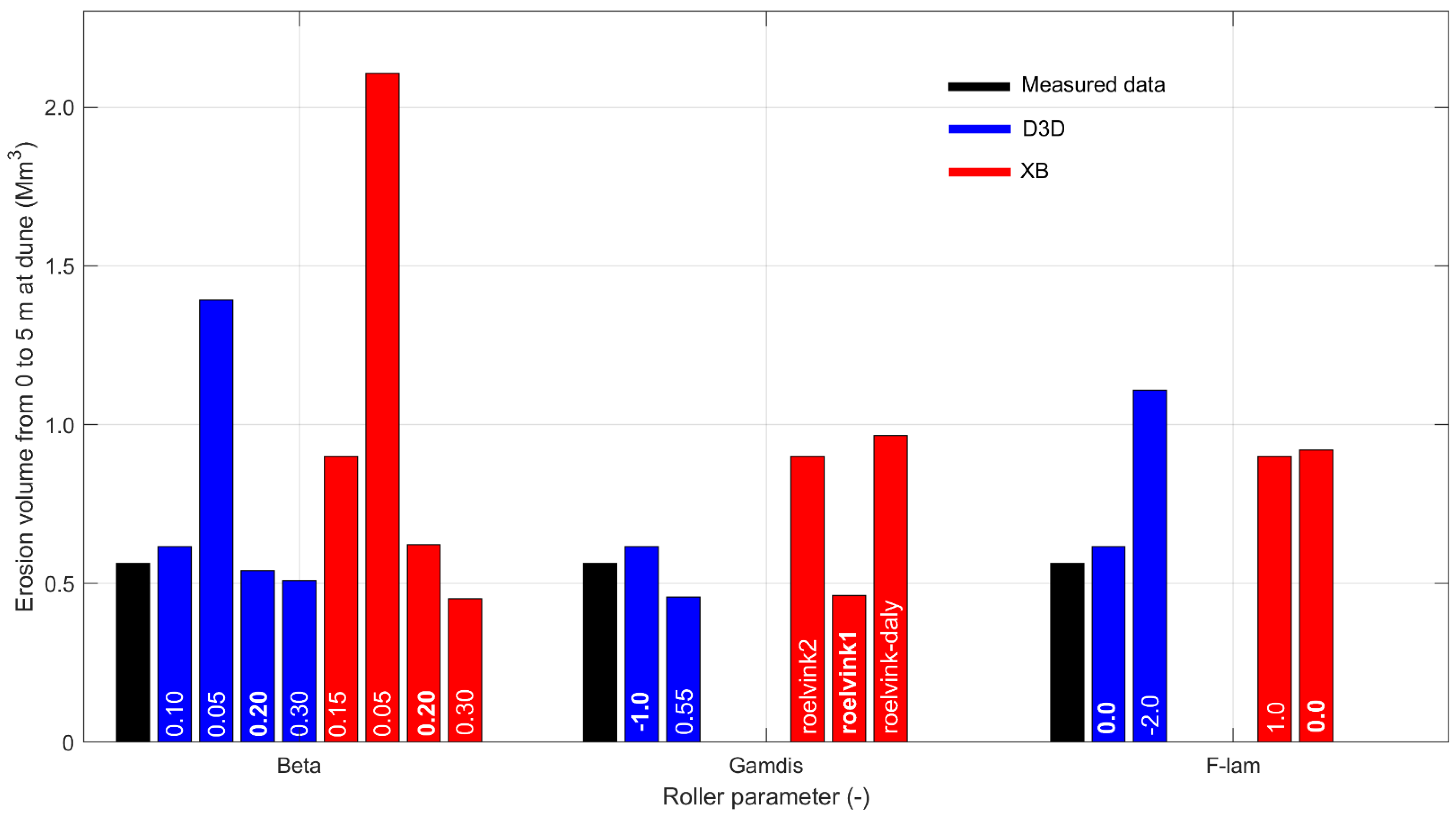
4.3.1. Sensitivity of Storm Erosion to Roller Dynamics
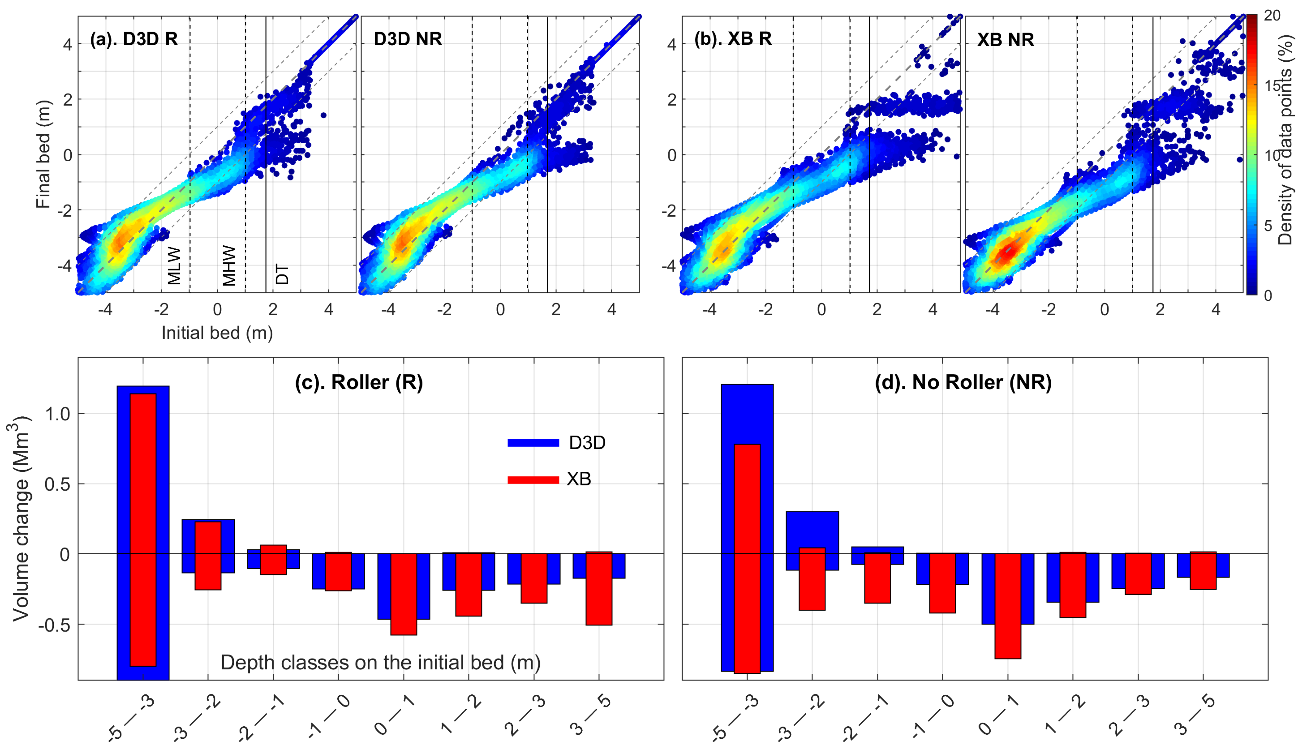
4.3.2. Roller Effect on Storm Erosion
5. Discussion
5.1. Hydrodynamics
5.2. Sensitivity of Roller Parameters
5.3. Roller Effect on Storm Erosion
5.4. Model Applications
6. Conclusions
Author Contributions
Funding
Institutional Review Board Statement
Informed Consent Statement
Data Availability Statement
Acknowledgments
Conflicts of Interest
Appendix A

| Process | Delft3D | XBeach | |
|---|---|---|---|
| Hydrodynamics | Wave model | Stationary (SWAN), Non-Stationary (Roller) | Non-Stationary (Surfbeat) |
| Wave from model nesting | ✓ | × | |
| Short-wave at boundary | ✓ | ✓ | |
| Long-wave at boundary | × | ✓ | |
| Short-wave spectrum | Jonswap | Jonswap | |
| Lateral wave boundary | × | wavecrest | |
| Wave computation | Direction/frequency | Direction domain only | |
| Wave breaking index | 0.73 (SWAN), −1 (Roller) | roelvink1 | |
| Lateral flow boundary | Neumann | Neumann | |
| Wave current interaction | ✓ | ✓ | |
| Bed friction—flow | C = 55 m1/2/s | 55 m1/2/s | |
| Bed friction—wave: SWAN | 0.067 m2/s−3 | × | |
| Bed friction—wave: Roller (fw) | 0 | 0 | |
| Roller dissipation coefficient (αrol) | 1 | 1 | |
| Time step | 6 s | CFL = 0.7 | |
| Communication with wave | 30 min | in-build | |
| Min. depth for Undertow (hmin) | × | 0.2 m | |
| Horizontal eddy viscosity | 0.1 m2/s | 0.1 m2/s | |
| Horizontal eddy diffusivity | 1.0 m2/s | 1.0 m2/s | |
| Sediment transport | Bed Sediment | Single fraction (300 µm) | Single fraction (300 µm) |
| Sediment layer | 5 m | 5 m | |
| Transport formula | Soulsby-Van Rijn | Soulsby-Van Rijn | |
| Bed slope | αbs = 1, αbn = 1.5 | roelvink_total | |
| Effect of wave Asymmetry | fsusw = 1, fbedw = 1 | fAs = 0.1 | |
| Effect of wave Skewness | × | fSk = 0.1 | |
| Morphological changes | Morphological acceleration | morfac = 1 | morfac = 1 |
| morfac option | × | 1 | |
| Avalanching | wetslope = 0.3 | wetslope = 0.3, dryslope = 1 | |
| Avalanching time | 1 day | × | |
| Dry Cell erosion (ThetSD) | 1 | - | |
References
- Harley, M.D.; Ciavola, P. Managing local coastal inundation risk using real-time forecasts and artificial dune placements. Coast. Eng. 2013, 77, 77–90. [Google Scholar] [CrossRef]
- Dissanayake, P.; Brown, J.; Sibbertsen, P.; Winter, C. Using a two-step framework for the investigation of storm impacted beach and dune erosion. Coast. Eng. 2021, 168, 103939. [Google Scholar] [CrossRef]
- Kron, W. Coasts: The high-risk areas of the world. Nat. Hazards 2013, 66, 1363–1382. [Google Scholar] [CrossRef]
- Dissanayake, P.; Brown, J.; Wisse, P.; Karunarathna, H. Effect of storm clustering on beach and dune evolution. Mar. Geol. 2015, 370, 63–75. [Google Scholar] [CrossRef]
- Huang, S.Y.; Yen, J.Y.; Wu, B.L.; Shih, N.W. Field observations of sediment transport across the rocky coast of east Taiwan: Impacts of extreme waves on the coastal morphology by Typhoon Soudelor. Mar. Geol. 2020, 421, 106088. [Google Scholar] [CrossRef]
- McGranahan, G.; Balk, D.; Anderson, B. The rising tide: Assessing the risks of climate change and human settlements in low elevation coastal zones. Environ. Urban 2007, 19, 17–37. [Google Scholar] [CrossRef]
- Neumann, B.; Vafeidis, A.T.; Zimmermann, J.; Nicholls, R.J. Future coastal population growth and exposure to sea-level rise and coastal flooding—A global assessment. PLoS ONE 2015, 10, e0131375. [Google Scholar] [CrossRef] [Green Version]
- De Jong, F.; Bakker, J.F.; van Berkel, C.J.M.; Dankers, N.M.J.A.; Dahl, K.; Gätje, C.; Marencic, H.; Potel, P. Wadden Sea Quality Status Report, 1999; Wadden Sea Ecosystem No. 9; Common Wadden Sea Secretariat, Trilateral Monitoring and Assessment Group, Quality Status Report Group: Wilhelmshaven, Germany, 1999. [Google Scholar]
- Sallenger, A. Storm impact scale for barrier islands. J. Coast. Res. 2000, 16, 890–895. [Google Scholar]
- Roelvink, D.; McCall, R.; Mehvar, S.; Nederhoff, K. Improving predictions of swash dynamics in XBeach: The role of groupiness and incident-band runup. Coast. Eng. 2018, 134, 103–123. [Google Scholar] [CrossRef]
- Roelvink, D.; Reniers, A.; van Dongeren, A.; van Thiel de Vries, J.; McCall, R.; Lescinski, J. Modelling storm impacts on beaches, dunes and barrier islands. Coast. Eng. 2009, 56, 1133–1152. [Google Scholar] [CrossRef]
- Lesser, G.; Roelvink, J.A.; van Kester, J.A.T.M.; Stelling, G.S. Development and validation of a three-dimensional morphological model. Coast. Eng. 2004, 51, 883–915. [Google Scholar] [CrossRef]
- Hsu, Y.L.; Dykes, J.D.; Allard, R.A. Evaluation of Delft3D Performance in Nearshore Flows; MS 39529-5004, NRL/MR/7320-06-8984; Naval Research Laboratory: Stennis Space Center, Hancock, MI, USA, 2006. [Google Scholar]
- Hsu, Y.L.; Dykes, J.D.; Allard, R.A. Validation Test Report for Delft3D; MS 39529-5004, NRL/MR/7320-08-9079; Naval Research Laboratory: Stennis Space Center, Hancock, MI, USA, 2008. [Google Scholar]
- Giardino, A.; Van der Werf, J.; Van Ormondt, M. Simulating Coastal Morphodynamics with Delft3D: Case Study Egmond aan Zee, Deltares Delft Hydraulics; 1200635-005; Deltares: Delft, The Netherlands, 2010. [Google Scholar]
- Smallegan, S.M.; Irish, J.L.; Van Dongeren, A.R.; Den Bieman, J.P. Morphological response of a sandy barrier island with a buried seawall during Hurricane Sandy. Coast. Eng. 2016, 110, 102–110. [Google Scholar] [CrossRef] [Green Version]
- Kalligeris, N.; Smit, P.B.; Ludka, B.C.; Guza, R.T.; Gallien, T.W. Calibration and assessment of process-based numerical models for beach profile evolution in southern California. Coast. Eng. 2020, 158, 103650. [Google Scholar] [CrossRef] [Green Version]
- Blossier, B.; Bryan, K.R.; Daly, C.J.; Winter, C. Spatial and temporal scales of shoreline morphodynamics derived from video camera observations for the island of Sylt, German Wadden Sea. Geo Mar. Lett. 2017, 37, 111–123. [Google Scholar] [CrossRef]
- Dissanayake, P.; Winter, C. Modelling the coastline orientation on storm erosion at the Sylt island, North Sea. In Proceedings of the Virtual Conference of Coastal Engineering, Sydney, Australia, 6–9 October 2020; Volume 36, p. 20. [Google Scholar]
- Ahrendt, K. Expected effect of climate change of Sylt island: Results from a multidisciplinary German project. Clim. Res. 2001, 18, 141–146. [Google Scholar] [CrossRef]
- Chu, K.; Winter, C.; Hebbeln, D.; Schulz, M. Improvement of morphodynamic modelling of tidal channel migration by nudging. Coast. Eng. 2013, 77, 1–13. [Google Scholar] [CrossRef]
- Van Ormondt, M.; Nelson, T.R.; Hapke, C.J.; Roelvink, D. Morphodynamic modelling of the wilderness breach, Fire Island, New York. Part I: Model set-up and validation. Coast. Eng. 2020, 157, 103621. [Google Scholar] [CrossRef]
- Stelling, G.S. On the construction of computational methods for shallow water flow problem. In Rijkswaterstaat Communications; Governing Printing Office: Hague, The Netherlands, 1984; Volume 35. [Google Scholar]
- Stelling, G.S.; Lendertse, J.J. Approximation of Convective Processes by Cyclic ACI methods. In Proceedings of the 2nd ASCE Conference on Estuarine and Coastal Modelling, Tampa, FL, USA, 13–15 November 1991. [Google Scholar]
- Booij, N.; Ris, R.C.; Holthuijsen, L.H. A third-generation wave model for coastal regions, Part I, Model description and validation. J. Geophys. Res. 1999, 104, 7649–7666. [Google Scholar] [CrossRef] [Green Version]
- Soulsby, R. Dynamics of marine sands, A manual for practical applications. Oceanogr. Lit. Rev. 1997, 9, 947. [Google Scholar]
- Holthuijsen, L.H.; Booij, N.; Herbers, T.H.C. A prediction model for stationary short-crested waves in shallow water with ambient currents. Coast. Eng. 1989, 13, 23–54. [Google Scholar] [CrossRef]
- Stelling, G.S.; Duinmeijer, S.P.A. A staggered conservative scheme for every Froude number in rapidly varied shallow water flows. Int. J. Numer. Methods Fluids 2003, 43, 1329–1354. [Google Scholar] [CrossRef]
- Ruggiero, P.; Walstra, D.J.R.; Gelfenbaum, G.; van Ormondt, M. Seasonal-scale nearshore morphological evolution: Field observations and numerical modeling. Coast. Eng. 2009, 56, 1153–1172. [Google Scholar] [CrossRef]
- Roelvink, J.A. Dissipation in random wave groups incident on a beach. Coast. Eng. 1993, 19, 127–150. [Google Scholar] [CrossRef]
- Brière, C.; Walstra, D.J.R. Modelling of Bar Dynamics; Report Z4099; WLlDelft Hydraulics: Delft, The Netherlands, 2006. [Google Scholar]
- Ruessink, B.G.; Walstra, D.J.R.; Southgate, H.N. Calibration and verification of a parametric wave model on barred beaches. Coast. Eng. 2003, 48, 139–149. [Google Scholar] [CrossRef]
- Daly, C.; Roelvink, J.A.; Van Dongeren, A.R.; Van Thiel de Vries, J.S.M.; McCall, R.T. Short wave breaking effects on low frequency waves. In Proceedings of the 32th International Conference on Coastal Engineering, Shanghai, China, 30 June–5 July 2010; pp. 1–13. [Google Scholar]
- Roelvink, J.A.; Meijer, T.J.G.P.; Houwman, K.; Bakker, R.; Spanhoff, R. Field validation and application of a coastal profile model. In Proceedings of the Coastal Dynamics Conference, Gdansk, Poland, 4–8 September 1995; pp. 818–828. [Google Scholar]
- Walstra, D.J.R.; Van Ormondt, M.; Roelvink, J.A. Shoreface Nourishment Scenarios; WL|Delft Hydraulics Report Z3748.21; Deltares: Delft, The Netherlands, 2004. [Google Scholar]
- Dissanayake, D.M.P.K. Modelling Morphological Response of Large Tidal Inlet Systems to Sea Level Rise; Taylor & Francis Group, CRC Press/Balkema: Leiden, The Netherlands, 2011; ISBN 978-0-415-62100-7. [Google Scholar]
- Dissanayake, P.; Yates, M.L.; Suanez, S.; Floc’h, F.; Krämer, K. Climate Change impacts on coastal wave dynamics at Vougot Beach, France. J. Mar. Sci. Eng. 2021, 9, 1009. [Google Scholar] [CrossRef]
- Donelan, M.A.; Hamilton, H.; Hui, W.H. Directional spectra of wind-generated waves. Philos. Trans. R. Soc. Lond. A 1985, 315, 509–562. [Google Scholar]
- Hasselmann, K.; Barnett, T.P.; Bouws, F.; Carlson, H.; Cartwright, D.E.; Enke, K.; Ewing, J.A.; Gienapp, H.; Hasselmann, D.E.; Krusemann, P.; et al. Measurements of Windwave Growth and Swell Decay during the Joint North Sea Wave Project (JONSWAP); Deutches Hydrographisches Institut, A8: Hamburg, Germany, 1973; pp. 1–95. [Google Scholar]
- Goda, Y. Random Seas and Design of Maritime Structures, Advanced series on Ocean Engineering 33, 3rd ed.; World Scientific: Jokohama, Japan, 2010. [Google Scholar]
- Fredsøe, J. Turbulent boundary layer in wave-current interaction. J. Hydraul. Eng. 1984, 110, 1103–1120. [Google Scholar] [CrossRef]
- Ruessink, B.G.; Miles, J.R.; Feddersen, F.; Guza, R.T.; Elgar, S. Modeling the alongshore current on barred beaches. J. Geophys. Res. 2001, 106, 451–463. [Google Scholar] [CrossRef]
- Krause, P.; Boyle, D.P.; Bäse, F. Comparison of different efficiency criteria for hydrological model assessment. Adv. Geosci. 2005, 5, 89–97. [Google Scholar] [CrossRef] [Green Version]
- Walstra, D.J.R. Unibest-TC User Guide. Report Z2897; WLlDelft Hydraulics: Delft, The Netherlands, 2000. [Google Scholar]
- Boyd, S.C.; Weaver, R.J. Replacing a third-generation wave model with a fetch based parametric solver in coastal estuaries. Estuar. Coast. Shelf Sci. 2021, 251, 107192. [Google Scholar] [CrossRef]
- Giardino, A.; Brière, C.; Van der Werf, J. Morphological Modelling of Bar Dynamics with Delft3D, the Quest for Optimal Parameter Settings; 1202345-000; Deltare: Delft, The Netherlands, 2011. [Google Scholar]
- Dissanayake, D.M.P.K.; Ranasinghe, R.; Roelvink, J.A. The morphological response of large tidal inlet/basin systems to relative sea level rise. Climate Change 2012, 113, 253–276. [Google Scholar] [CrossRef] [Green Version]
- Elmilady, H.; Van der Wegen, M.; Roelvink, D.; Van der Spek, A. Morphodynamic Evolution of a Fringing Sandy Shoal: From Tidal Levees to Sea Level Rise. JGR Earth Surface 2020, 125, e2019JF005397. [Google Scholar] [CrossRef]


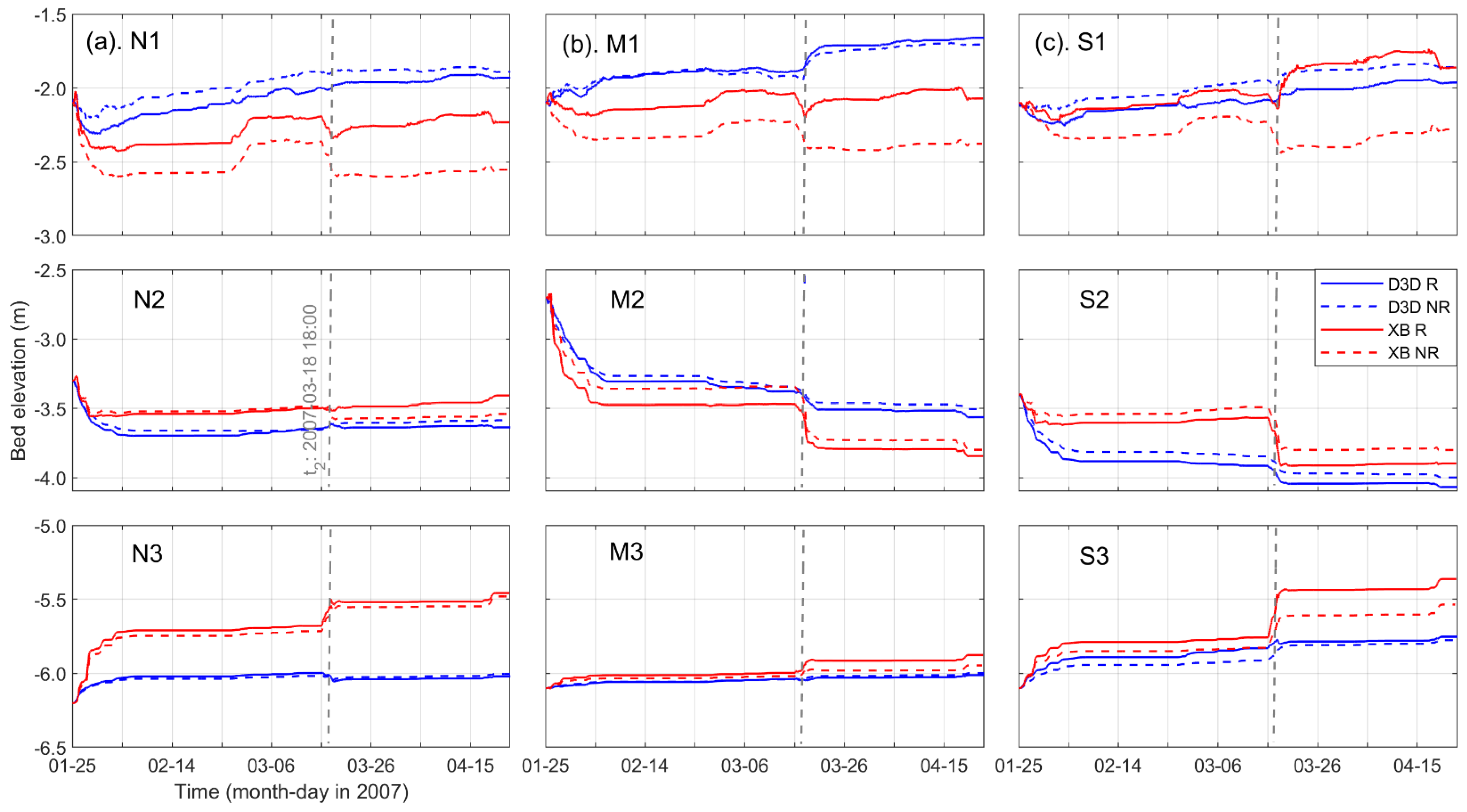
| Location | Distance from MSL (m) | Depth (m) | |
|---|---|---|---|
| North (N) | N1 | 58 | 2.1 |
| N2 | 233 | 3.3 | |
| N3 | 481 | 6.2 | |
| Middle (M) | M1 | 67 | 2.1 |
| M2 | 285 | 2.7 | |
| M3 | 531 | 6.1 | |
| South (S) | S1 | 86 | 2.1 |
| S2 | 356 | 3.4 | |
| S3 | 513 | 6.1 | |
| Physical Process | D3D | XB | |||
|---|---|---|---|---|---|
| R | NR | R | NR | ||
| Short-wave | ✓ | ✓ | ✓ | ✓ | |
| Long-wave from offshore | × | × | ✓ | ✓ | |
| Long-wave effect from short wave breaking (roller model) | ✓ | × | ✓ | × | |
| Wave computation | Directional-Domain | ✓ | ✓ | ✓ | ✓ |
| Frequency-Domain | ✓ | ✓ | × | × | |
| Undertow | × | × | ✓ | ✓ | |
| Avalanching | ✓ | ✓ | ✓ | ✓ | |
| Model Domain | Spatial Extent (Cross Shore × Alongshore in km) | Grid Nodes | Range of Grid Resolution (Cross Shore × Alongshore in m) |
|---|---|---|---|
| apex-grid | 9.8 × 15 | 15,120 | 4–200 × 190–300 |
| west-grid | 10.2 × 38 | 7857 | 8–400 × 400–600 |
| Scenario | D3D | XB | No. of Simulations | |||
|---|---|---|---|---|---|---|
| R | NR | R | NR | |||
| Hydrodynamics only | ✓ | ✓ | ✓ | ✓ | 4 | |
| Sensitivity analysis | Beta | 0.10 | 0.15 | 8 | ||
| 0.05 | 0.05 | |||||
| 0.20 | 0.20 | |||||
| 0.30 | 0.30 | |||||
| Gamdis | −1 | roelvink2 | 5 | |||
| 0.55 | roelvink1 | |||||
| roelvink_daly | ||||||
| F_lam | 0 | 1 | 4 | |||
| −2 | 0 | |||||
| Beach and dune erosion | ✓ | ✓ | ✓ | ✓ | 4 | |
| Source | Wave Height | Wave Spectral Density (SD) | ||
|---|---|---|---|---|
| R2 (-) | RMSE (m) | ∑SD (kJ/m2/Hz) | µ (-) | |
| Observations (Hs) | - | - | 8.99 | - |
| D3D (Hs) | 0.91 | 0.14 | 8.67 | −0.03 |
| XB (Hrms) | 0.83 | 0.21 | 6.47 | −0.27 |
| XB (Hs) | 0.83 | 0.26 | 12.95 | 0.45 |
| Location | <Wave Height> (m) | <|Velocity|> (m/s) | <|Bed Shear Stress|> (m/s) | ||||||||||||
|---|---|---|---|---|---|---|---|---|---|---|---|---|---|---|---|
| D3D Hs | XB Hrms | XB Hs | D3D | XB | D3D | XB | |||||||||
| R | NR | R | NR | R | NR | R | NR | R | NR | R | NR | R | NR | ||
| North (N) | N1 | 0.71 | 0.78 | 0.65 | 0.65 | 0.92 | 0.92 | 0.30 | 0.25 | 0.26 | 0.28 | 0.74 | 0.54 | 0.81 | 0.90 |
| N2 | 0.79 | 0.87 | 0.68 | 0.68 | 0.96 | 0.96 | 0.20 | 0.18 | 0.15 | 0.15 | 0.32 | 0.24 | 0.32 | 0.32 | |
| N3 | 0.89 | 0.97 | 0.68 | 0.68 | 0.96 | 0.96 | 0.21 | 0.20 | 0.18 | 0.18 | 0.24 | 0.22 | 0.22 | 0.22 | |
| Middle (M) | M1 | 0.69 | 0.78 | 0.66 | 0.66 | 0.94 | 0.94 | 0.29 | 0.24 | 0.23 | 0.24 | 0.66 | 0.48 | 0.67 | 0.71 |
| M2 | 0.76 | 0.88 | 0.67 | 0.67 | 0.95 | 0.95 | 0.22 | 0.20 | 0.19 | 0.19 | 0.38 | 0.29 | 0.28 | 0.27 | |
| M3 | 0.90 | 0.99 | 0.70 | 0.70 | 0.99 | 0.99 | 0.25 | 0.24 | 0.23 | 0.23 | 0.33 | 0.29 | 0.29 | 0.29 | |
| South (S) | S1 | 0.66 | 0.70 | 0.66 | 0.66 | 0.93 | 0.93 | 0.28 | 0.23 | 0.19 | 0.20 | 0.66 | 0.45 | 0.57 | 0.59 |
| S2 | 0.78 | 0.84 | 0.68 | 0.68 | 0.96 | 0.96 | 0.20 | 0.18 | 0.15 | 0.15 | 0.35 | 0.25 | 0.31 | 0.31 | |
| S3 | 0.85 | 0.91 | 0.69 | 0.68 | 0.97 | 0.97 | 0.18 | 0.17 | 0.16 | 0.16 | 0.20 | 0.16 | 0.19 | 0.19 | |
| Roller Parameter | D3D | XB | ||||||
|---|---|---|---|---|---|---|---|---|
| Value | N | M | S | Value | N | M | S | |
| Beta | 0.10 | 1.69 | 0.96 | 1.69 | 0.15 | 1.78 | 2.18 | 1.46 |
| 0.05 | 1.83 | 1.14 | 1.79 | 0.05 | 1.97 | 2.35 | 1.55 | |
| 0.20 | 1.54 | 0.88 | 1.65 | 0.20 | 1.75 | 2.17 | 1.41 | |
| 0.30 | 1.51 | 0.90 | 1.63 | 0.30 | 1.73 | 2.15 | 1.43 | |
| Gamdis | −1 | 1.69 | 0.96 | 1.69 | roelvink2 | 1.78 | 2.18 | 1.46 |
| 0.55 | 1.34 | 0.67 | 1.26 | roelvink1 | 1.66 | 1.92 | 1.24 | |
| roelvink_daly | 2.01 | 2.17 | 1.77 | |||||
| F_lam | 0 | 1.69 | 0.96 | 1.69 | 1 | 1.78 | 2.18 | 1.46 |
| −2 | 1.93 | 1.32 | 1.90 | 0 | 1.77 | 2.20 | 1.44 | |
| Roller Parameter | Value | |
|---|---|---|
| D3D | XB | |
| Beta | 0.20 | 0.20 |
| Gamdis | −1.0 | roelvink1 |
| F_lam | 0.0 | 0.0 |
| Depth Class (m) | D3D | XB |
|---|---|---|
| −5 to −3 | 0.18 | −0.06 |
| −3 to −2 | 0.15 | −0.36 |
| −2 to −1 | 0.31 | −0.58 |
| −1 to 0 | 0.11 | −0.38 |
| 0 to 1 | −0.06 | −0.22 |
| 1 to 2 | −0.22 | −0.02 |
| 2 to 3 | −0.05 | 0.21 |
| 3 to 5 | 0.13 | 0.97 |
Publisher’s Note: MDPI stays neutral with regard to jurisdictional claims in published maps and institutional affiliations. |
© 2022 by the authors. Licensee MDPI, Basel, Switzerland. This article is an open access article distributed under the terms and conditions of the Creative Commons Attribution (CC BY) license (https://creativecommons.org/licenses/by/4.0/).
Share and Cite
Dissanayake, P.; Brown, J. Modelling the Effect of ‘Roller Dynamics’ on Storm Erosion: Sylt, North Sea. J. Mar. Sci. Eng. 2022, 10, 305. https://doi.org/10.3390/jmse10030305
Dissanayake P, Brown J. Modelling the Effect of ‘Roller Dynamics’ on Storm Erosion: Sylt, North Sea. Journal of Marine Science and Engineering. 2022; 10(3):305. https://doi.org/10.3390/jmse10030305
Chicago/Turabian StyleDissanayake, Pushpa, and Jennifer Brown. 2022. "Modelling the Effect of ‘Roller Dynamics’ on Storm Erosion: Sylt, North Sea" Journal of Marine Science and Engineering 10, no. 3: 305. https://doi.org/10.3390/jmse10030305
APA StyleDissanayake, P., & Brown, J. (2022). Modelling the Effect of ‘Roller Dynamics’ on Storm Erosion: Sylt, North Sea. Journal of Marine Science and Engineering, 10(3), 305. https://doi.org/10.3390/jmse10030305