A Multi-Proxy Approach to Reconstruct Hypoxia on the NW Black Sea Shelf over the Holocene

Abstract

Coastal hypoxia is a worldwide concern. Even though seasonal hypoxia has been reported on the northwestern Black Sea shelf since the 1970s, little is known about oxygenation in this area over the Holocene. With a multiproxy approach, this work aimed to detect potential hypoxic events in two gravity cores. Our results demonstrate that the most common proxies of hypoxia are irrelevant for the Black Sea coastal environment. For instance, the Ammonia-Elphidium index appears to be inappropriate. We assume a salinity bias due to the influence of freshwater inputs. Likely, the redox sensitivity of vanadium is obscured by the dominant supply of detrital elements. However, the size distribution of framboidal pyrites gives clear indications of the oxygenation of the water column. Indeed, the absence of framboidal pyrites in the core located at the Danube mouth suggests permanent oxic conditions over the last 2 ka. On the contrary, in the core located in the Odessa Bay, the two observed ranges of pyrite sizes evidence an alternation between anoxic (mean diameter 3–6 ± 1–2 µm) and hypoxic or oxic (mean diameter 6–10 ± 3–5 µm) conditions in bottom waters over the last 7 ka. Therefore, this proxy reveals different oxygenation levels for these proximal sites.

1. Introduction

In the global ocean, dissolved oxygen plays an essential role in aerobic respiration and thus in ecosystem equilibrium, biodiversity preservation and organic matter degradation. Moreover, oxygen interacts with biogeochemical cycles. Currently, ocean deoxygenation is a growing concern: decreasing oxygen concentration in different types of marine environments affects fisheries and consequently the economy and food safety. The increase in oxygen loss is attributed to climatic warming and excessive nutrient discharges to the coastal area [1]. The decline in oxygen concentration concerns mainly the oxygen minimum zones (OMZs), fjords, coastal areas and restricted marine basins such as the Baltic Sea or the Black Sea. In situ measurements of oxygen concentration show an increase in the size of areas affected by oxygen depletion and in the duration of these low-oxygen conditions [1].

There are different terms used to define the levels of deoxygenation. Anoxia refers to the total absence of oxygen, while the term hypoxia is used when the oxygen level is sufficiently low to badly affect most organisms. As the tolerance of each species is different, a threshold of 2 mg L⁻¹ of oxygen (63 µmol L⁻¹) has been chosen [1,2]. Hypoxia can occur at variable frequencies and durations [3], but is seasonal in half of the documented cases [2].

Studies of the Black Sea deep basin have often focused on the establishment and intensity of anoxia [4,5,6] as well as on the oscillations of the chemocline separating oxygenated surface waters from anoxic and hydrogen sulphide-rich waters [7]. They have shown that the edge of the shelf can be submerged by anoxic water from the deep basin [8,9]. Although the long-term evolution of shelf oxygenation is not known, seasonal hypoxia has been recorded on the northwestern Black Sea shelf since the 1970s [10]. This shelf (<100 m deep) extends over 127,000 km² and receives large inputs of freshwater and nutrients via the Danube, the Dniestr, the Bug and the Dniepr [11], stimulating local primary production. During winter and spring, shelf bottom waters are well oxygenated due to the vertical mixing by storms and strong winds. In early summer, a thermal stratification (i.e., thermocline) sets in, and bottom waters are separated from surface waters. Below the thermocline, the oxic degradation of organic matter consumes oxygen along the stratified season, eventually reaching hypoxic or anoxic conditions by the end of summer or early autumn [12,13]. Although the current seasonal hypoxia is well studied, little is known about the occurrence of hypoxic events on the Black Sea shelf during the Holocene.

This work aims to reconstruct the history of oxygenation on the shelf using sedimentary cores. As the recent seasonal hypoxia was reported to develop, particularly near the coast [12], two coastal sites were chosen for this study. The oxygenation level of past bottom waters can be estimated with proxies, i.e., indicators influenced by the oxygen level and preserved in the sediment. Several biological, sedimentological and geochemical proxies have been proposed in the literature (see [14] for a review): the preserved remains of benthic and planktonic organisms (e.g., foraminifera), the sedimentary features (e.g., laminations), the chemistry and mineralogy of the sediment (e.g., sulphides and redox-sensitive trace elements), the pigments and lipid biomarkers, the organic C, N and their isotopic values. In this work, we tested some of the proxies (Figure 1) to detect past periods of oxygen depletion potentially recorded in the sediments of the NW Black Sea shelf. In the following section, the proxies selected in this study are first briefly reviewed. Then, the two studied sedimentary cores are described, and their age-depth models are presented. Results obtained from the different proxies are exposed. We finally discussed the usefulness of the different proxies in the context of the Black Sea shelf.

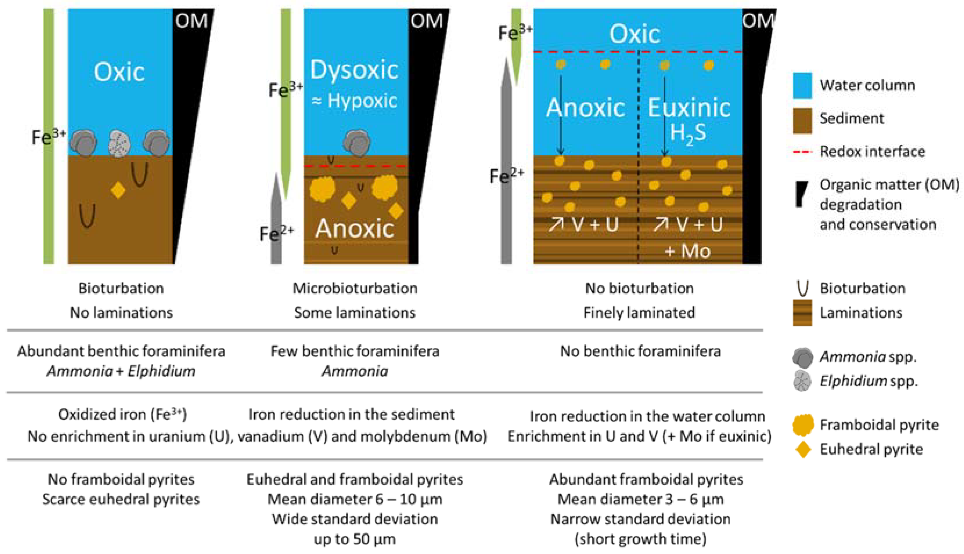
2. Potential Proxies for Bottom Water Oxygen Level

The following biological, geochemical and mineralogical proxies have been used in the literature to infer the oxygen level of bottom waters and were tested in this work. Among the proposed proxies, none is able to detect seasonal hypoxia given that a sediment sample corresponds to an average of several years and geochemical exchanges between the sediment and the overlying water occur continuously through sedimentation, bioturbation and benthic fluxes. Moreover, the sediment is affected by diagenesis and compaction after its deposition. Other parameters, for example, the sediment input, rate and resuspension, salinity variations and water stratification, might influence the proxies. In this study, the oxygenation level inferred from proxies was divided into four categories (Figure 1): oxic (well-oxygenated), dysoxic (moderate oxygen depletion, considered here as a synonym of hypoxic), anoxic (no oxygen) and euxinic (no oxygen with the presence of hydrogen sulphide).

2.1. Biological Proxy: Benthic Foraminifera

Organisms have different sensitivities with respect to oxygen depletion, and their identification in the sediment can indicate the evolution of the oxygen level over time. For example, Rabalais et al. [21] and Sen Gupta et al. [16] observed a relationship between oxygen content and foraminifera assemblage on the Gulf of Mexico shelf. Consequently, Sen Gupta et al. [16] developed the Ammonia-Elphidium index (here referred to as the A-E index). Ammonia species are known to be more resistant to oxygen restriction than most of the other foraminifera species and, in particular, those of the genus Elphidium (Figure 1). Thus, the A-E index allows one to identify the hypoxic events in shallow marine environments. The two genera are observed in large numbers in the Black Sea [22].

We use the A-E index proposed by Sen Gupta et al. [16]:

$$\mathrm{A}-\mathrm{E} \mathrm{index}=\left(\frac{{\mathrm{N}}_{\mathrm{A}}}{{\mathrm{N}}_{\mathrm{A}}+{ \mathrm{N}}_{\mathrm{E}}}\right)\times 100,$$

(1)

where N_A is the number of individuals from the genus Ammonia and N_E is the number of individuals from the genus Elphidium.

2.2. Sedimentological Proxies

The preservation of laminations indicates weak or even absent bioturbation by benthic organisms [14,15]. In the case of oxygen depletion in bottom waters, benthic organisms are less abundant or even absent under anoxic conditions. Thus, Zillén et al. [15] used laminated intervals in sediment cores from the Baltic Sea to detect past periods of hypoxia (Figure 1).

2.3. Geochemical Proxies

Organic matter content should be higher in the case of hypoxia (Figure 1) because the lack of oxygen leads to a high preservation of organic matter that is not degraded [17]. For example, in the Baltic Sea, hypoxic periods are characterised by peaks of organic carbon content (C_org, 5 to 10% and up to 15% in modern sediments) and oxic intervals by lower C_org content (2 to 3%) [23,24,25].

Redox-sensitive elements are used as geochemical proxies of hypoxia which corresponds to a reducing environment. In this work, trace metal enrichment and iron redox-state were investigated.

First, authigenic enrichment of redox-sensitive trace metals occurs under reducing conditions. In particular, vanadium (V) and uranium (U) are often used as proxies to detect anoxic conditions and molybdenum (Mo) to detect euxinic bottom waters [18].

Second, iron (Fe) is a redox-sensitive element. The oxidised iron (Fe III) is insoluble, while the reduced iron (Fe II) is soluble. Initially, iron is eroded and transported towards adjacent basins with detrital elements, such as aluminium (Al), silicon (Si), potassium (K) and titanium (Ti). If the redox conditions change during deposition or diagenesis, iron can be dissolved and precipitated again. This remobilisation of iron results in an iron signature in the sediment that is different from that of the detrital elements. A first approach is thus to test the correlation between iron and detrital elements with, for example, principal component analysis. Enrichment in iron has been used in several studies (e.g., [24]). For example, Spofforth et al. [26] consider that anoxia is indicated by a high Fe/Al ratio and high sulphur (S) content measured by an X-ray fluorescence (XRF) core scanner.

Moreover, the iron redox state can be determined by iron speciation (e.g., [27]). In the sediment, total Fe can be divided between non-reactive Fe (i.e., iron in silicates such as clay minerals) and reactive Fe (i.e., all iron species that interact in geochemical cycles).

2.4. Mineralogical Proxy: Framboidal Pyrites

Pyrite (FeS₂) forms under reducing conditions. Different pyrite morphologies can be encountered. Framboidal pyrite is the most abundant morphology in sediments and sedimentary rocks and consists of a spherical aggregate of pyrite micro-crystals in a raspberry-like form [28]. The usefulness of framboidal pyrites as a proxy for oxygen-level comes from the fact that the size of framboidal pyrites depends on the oxygen content of bottom waters [19]. The nucleation and the subsequent aggregation of micro-crystals occur just under the redox interface between oxygenated waters and hydrogen sulphide-rich waters, according to Wilkin and Barnes [4]. The size of the framboids depends on the growth time and, thus, the position of the redox interface. In the case of anoxic bottom waters, the redox interface is located in the water column (Figure 1). As framboidal pyrites sink rapidly after their formation due to their density, their growth time is limited, resulting in a smaller size [19]. On the contrary, if the redox interface is located within the sediment, framboidal pyrites have a longer growth time and are thus bigger [19]. Two diagnostic categories of size distributions can be highlighted. Firstly, if the mean diameter is between 3 and 6 µm with a narrow standard deviation, it corresponds to anoxic or euxinic bottom waters. Secondly, if the mean diameter is between 6 and 10 µm, including framboids up to 50 µm in parallel with a wider standard deviation, it indicates dysoxic or oxic bottom waters [19] (Figure 1). If no framboidal pyrites are found, it is interpreted as an indication of past oxic bottom waters [20] (Figure 1).

3. Materials and Methods

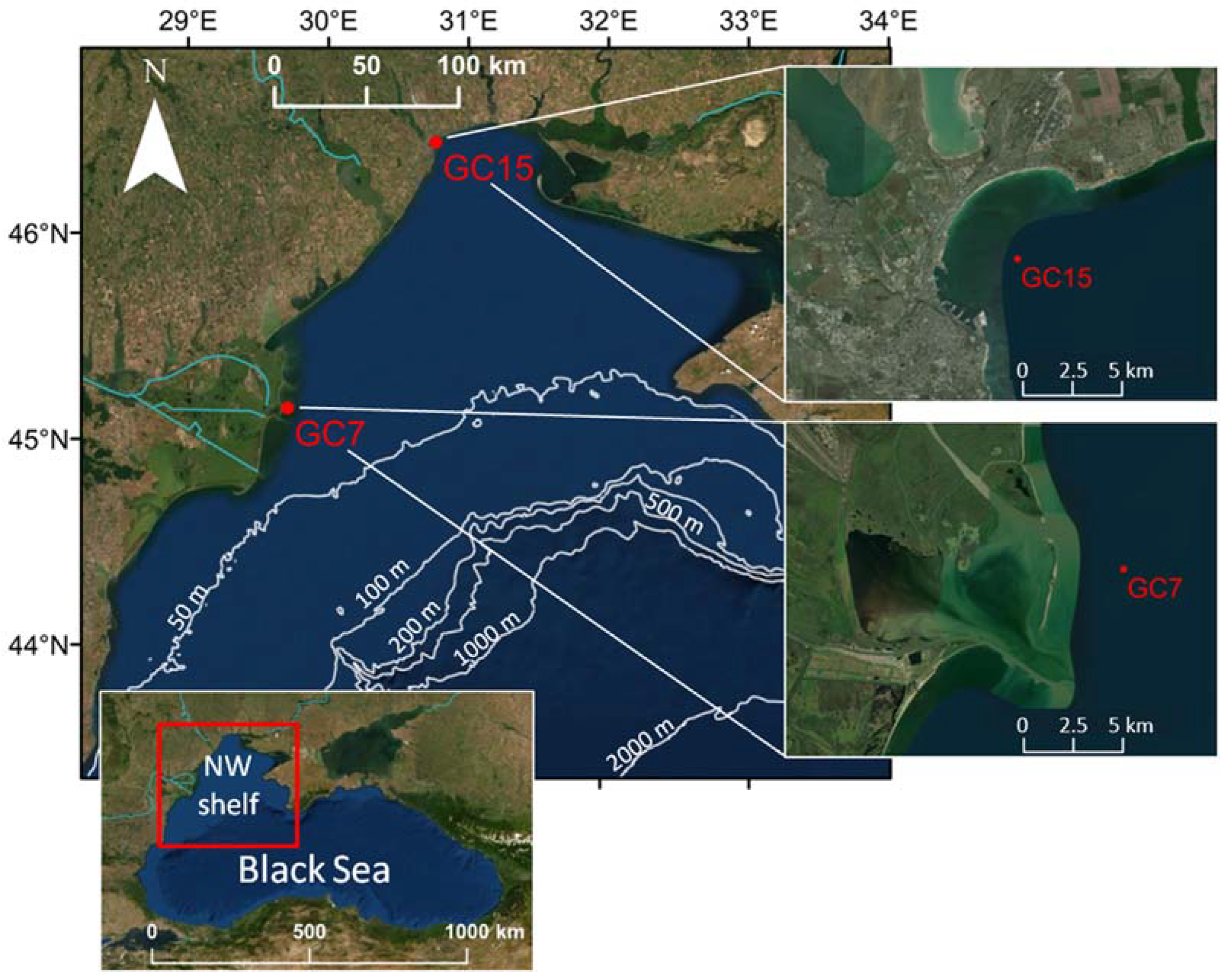
3.1. Study Sites

The two studied cores were retrieved in the framework of the BenthOx Project (FNRS PDR T.1009.15) by a gravity corer on board the RV Mare Nigrum in May 2016, during the EMBLAS-II cruise. Both cores are from the NW Black Sea shelf, less than 5 km from the coast (Figure 2). The MN16-GC7 core (215 cm long) was collected at the mouth of the Danube (at 20.5 m below sea level), and the MN16-GC15 core (297 cm long) was taken in the Odessa Bay (at 19 m below sea level). The gravity corer sampling method does not allow one to preserve the water-sediment interface. However, multicorers (MN16-MC7 and MN16-MC15) better preserve the water-sediment interface [29]. The core names are abbreviated as GC7, MC7, GC15 and MC15 in the following text.

3.2. Sampling Strategy and Sedimentological Methods

The cores of 10 cm in diameter were subdivided into two half-cylinders. Plastic sleeves (for X-radiographs and X-ray fluorescence core scanner) and 25 cm long metal boxes (for thin sections) were inserted into one half-cylinder. In the plastic sleeves, the 20 cm at the top of GC7 and 25 cm at the top of GC15 were not scanned. The other half-cylinder was sliced at every centimetre interval. Each slice was divided into four subsamples used for different proxy analyses: (1) the sedimentological analyses (X-ray diffraction and grain size analysis), (2) the geochemical analyses (quantitative measurements and reactive iron extraction), (3) the foraminifera and framboidal pyrite observations and (4) a reserve sample. For the proxy analyses, laminated intervals in GC7 and GC15 were targeted, given that these intervals were assumed to be more likely anoxic/hypoxic, according to Zillén et al. [15]. In addition, reworked shell layers (Units 3 and 5, see Figure 3) in GC15 were not sampled for further analyses. Finally, additional samples were taken in order to obtain a well-distributed sampling.

The description of the sedimentary cores is based on macroscopic observations, X-radiographs and thin sections. X-radiographs (SCOPIX) were performed by the EPOC laboratory (University of Bordeaux) on plastic sleeves using an X-ray source (microfocus 130 kV–L9181-02–HAMAMATSU) coupled with a detector (X-ray TDI camera C10650–HAMAMATSU) to obtain high-resolution images (0.92 mm) and the associated grey scale. The thin sections were performed by the EPOC laboratory (University of Bordeaux) and by MKfactory (Stahnsdorf, Germany).

Grain size analyses were performed at every 5 cm interval on 44 samples from GC7 and 27 from GC15 at the University of Liege, using a Malvern Mastersizer 2000 laser grain size analyser coupled to a Hydro S wet dispersion unit. The results were processed using the Mastersizer 2000 software.

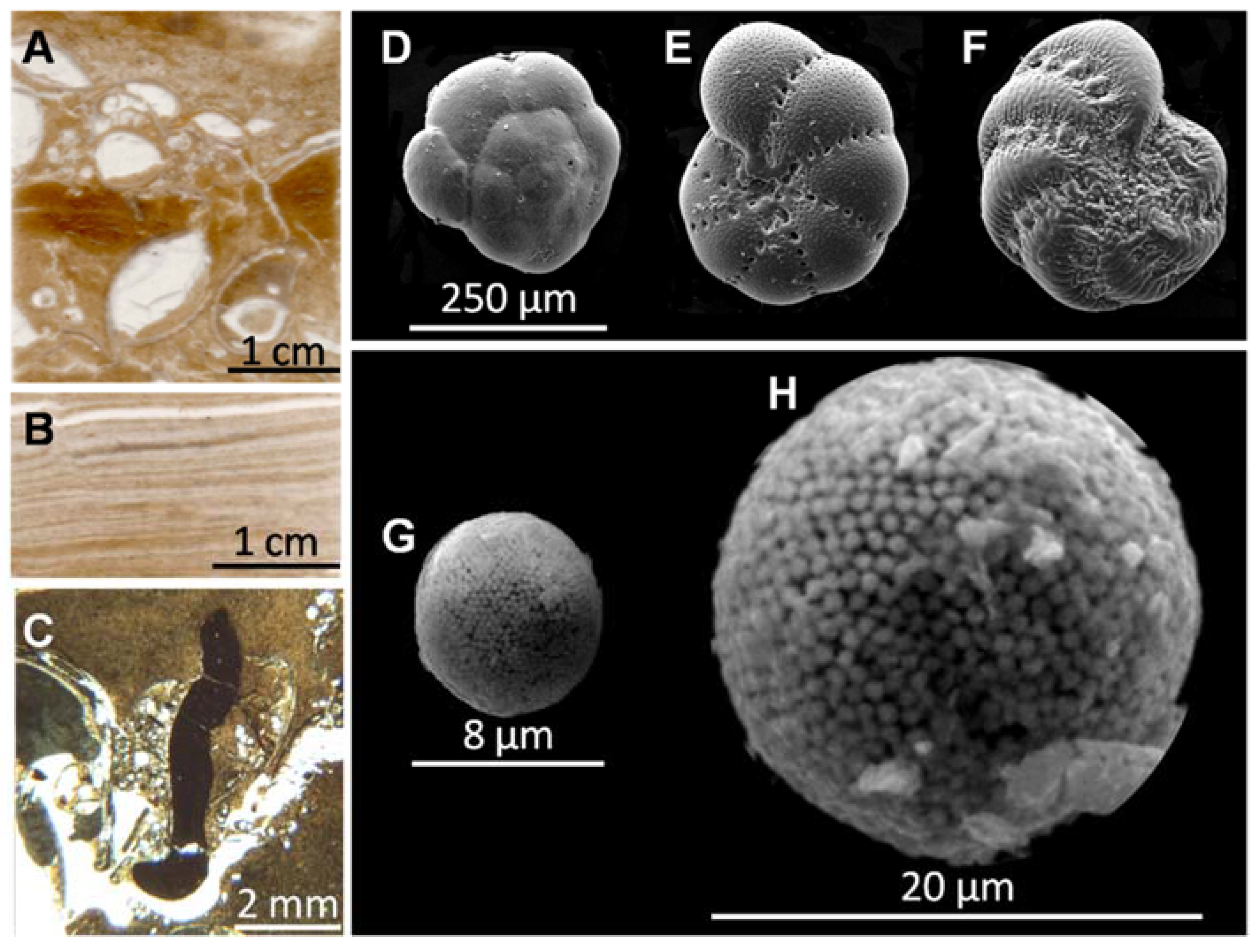
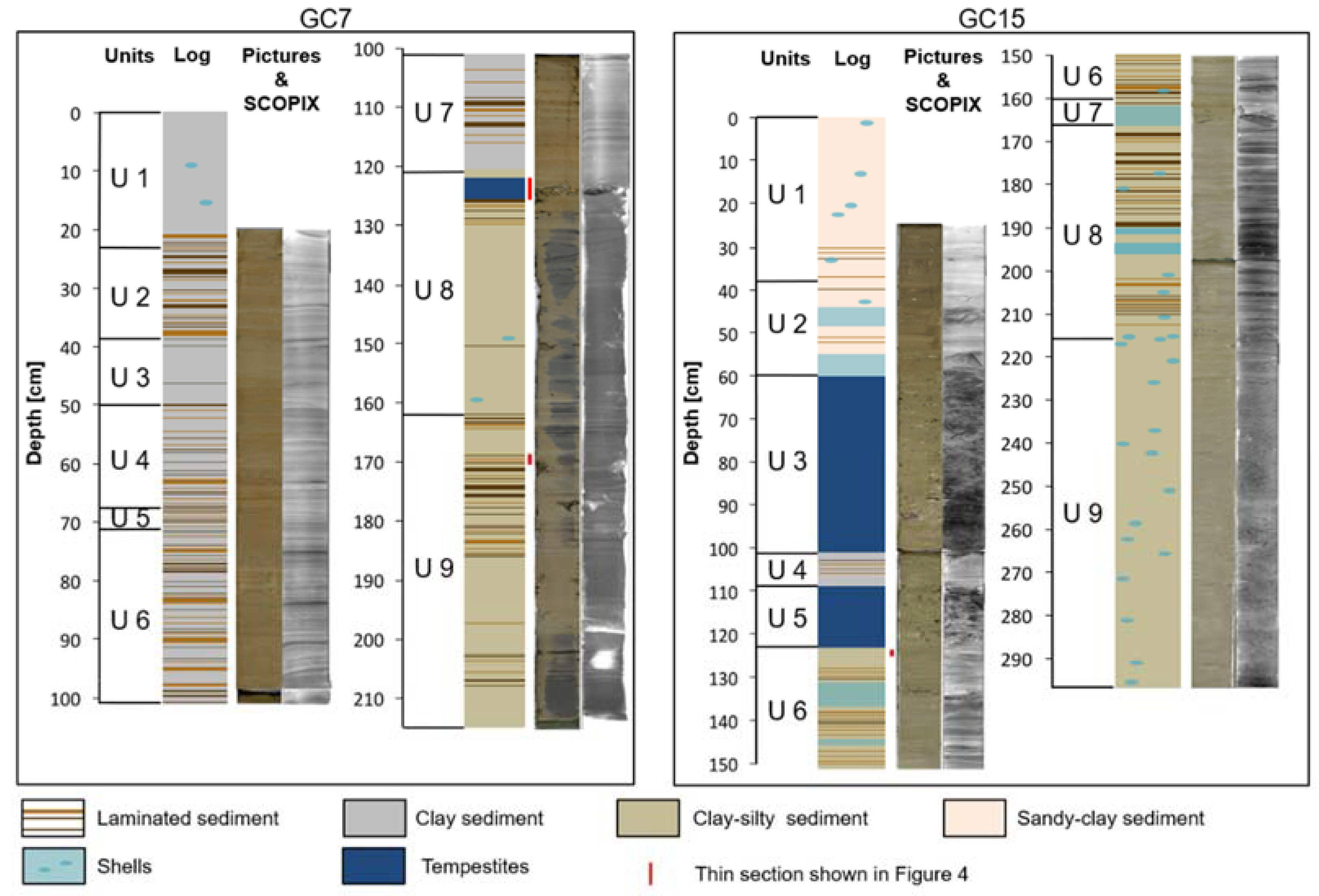
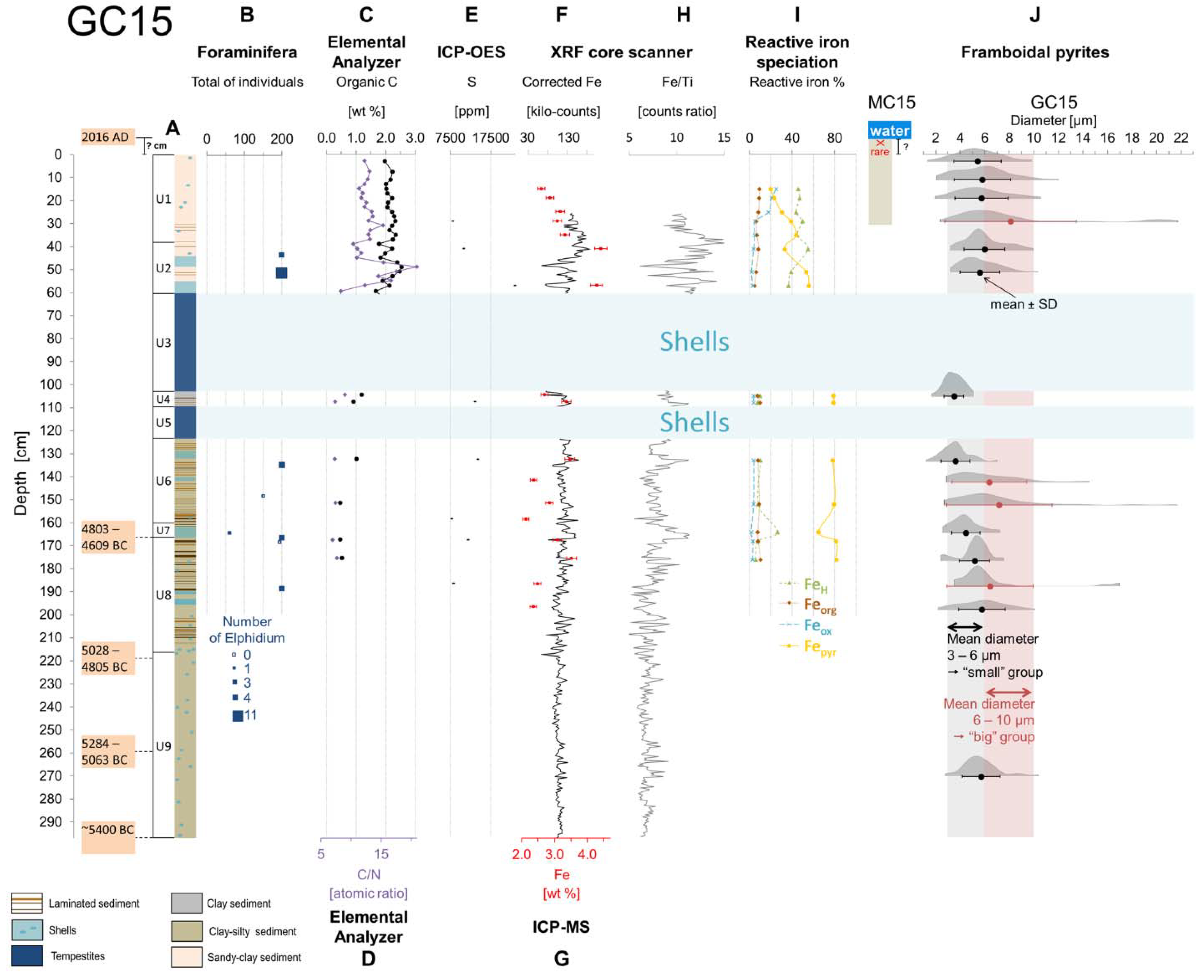
3.3. Description of the Cores and Sediment Characteristics

The upper part of the GC7 core (Figure 3) is composed of homogeneous clayey sediment, with laminated (Units 2, 4 to 7) and homogeneous units (Units 1 and 3). At greater depths (Units 8 and 9), coarser levels are interspersed with laminations and a graded shell level interpreted as a tempestite (i.e., storm deposits) at the top of Unit 8. The lamination thickness is millimetric to pluri-centimetric. The identified broken shells belong to bivalves, brachiopods and foraminifera.

In the GC15 core (Figure 3), Units 1 and 2 consist of homogeneous sandy-clay sediment with a few laminations. In Units 3 and 5, the sediment is mainly composed of broken and intact shells. These units are interpreted as multi-decimetric amalgamated tempestites. In the lower part of the core, Units 6 to 8 show laminated clay-silty sediments. The lamination thickness is millimetric to centimetric. A sharp transition is observed between the laminated Unit 8 and the homogeneous Unit 9. The latter has not been studied in detail. No lithological correlation between the two cores was possible since they are located 150 km from each other.

In the thin sections, several sedimentary structures were observed, such as tempestites (Figure 4A), geopetal structures, laminations (Figure 4B) and bioturbations (Figure 4C). Tempestites (top of Unit 8 in GC7 and Units 3 and 5 in GC15) highlight events, including storms, during which energy on the shelf is sufficient to remobilise sediment and shells in a large number. During this kind of energetic event, the water column is mixed. The bottom waters and the remobilised sediment are thus temporarily oxygenated. Moreover, geopetal structures have been observed. They show, in addition to the tempestites, significant remobilisation of the sediment. Numerous bioturbations were observed in thin sections, even in the macroscopically laminated levels. Thus, both cores were impacted by different perturbations and reworked at many depths over several centimetres, especially GC15 with a 40 cm-thick tempestite level (Figure 3, U3).

Figure 4. Illustrations of elements encountered in the studied cores. Sedimentary structures observed in thin section by optic microscope (see vertical positions in the cores in Figure 3): (A) tempestite at the top of Unit 8 in GC7; (B) laminations between 169 and 171 cm in GC7 (Unit 9) and (C) bioturbation between 145 and 146 cm in GC15 (Unit 6). Scanning electron microscopy (SEM) images of benthic foraminifera: (D) Ammonia spp. and (E,F) two different species of Elphidium spp. SEM images of framboidal pyrites: (G) between 1 and 5 cm and (H) between 28 and 30 cm in the GC15 core.

Figure 4. Illustrations of elements encountered in the studied cores. Sedimentary structures observed in thin section by optic microscope (see vertical positions in the cores in Figure 3): (A) tempestite at the top of Unit 8 in GC7; (B) laminations between 169 and 171 cm in GC7 (Unit 9) and (C) bioturbation between 145 and 146 cm in GC15 (Unit 6). Scanning electron microscopy (SEM) images of benthic foraminifera: (D) Ammonia spp. and (E,F) two different species of Elphidium spp. SEM images of framboidal pyrites: (G) between 1 and 5 cm and (H) between 28 and 30 cm in the GC15 core.

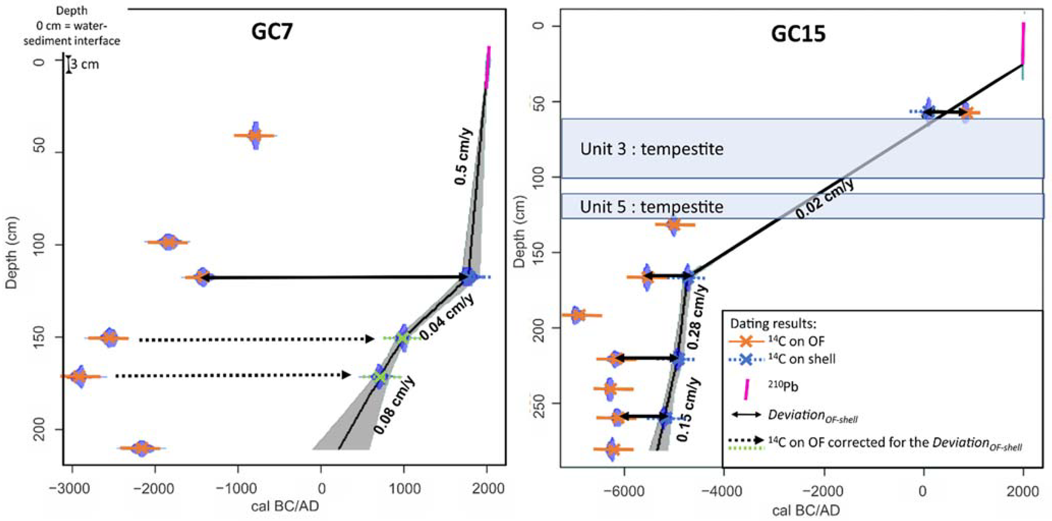
3.4. Core Chronology

For the most recent sediments, ²¹⁰Pb measurements were conducted on 3 samples from MC7 (at 0.5, 4 and 8 cm depths) and 6 samples from GC15 (at 0.5, 10.5, 20.5, 28, 32 and 34 cm depths). Results of ²¹⁰Pb dating are presented in

Table A1. Results of the ²¹⁰Pb dating on MC7 and GC15 by the EPOC laboratory (University of Bordeaux, France). The dating at 25 cm depth in GC15 was derived from the other ²¹⁰Pb dates carried out on GC15 samples. The dating was performed on the fine (<63 µm) organic fraction of the sediment (OF).

Core	Depth (cm)	Material Dated	210Pb cal BP	Error	Inferred Sedimentation Rate (cm/year)	Included in the Model Age
MC7	0.5	OF	2015	5	0.41	Yes
	4	OF	2006	5		Yes
	8	OF	1997	5		Yes
GC15	0.5	OF	2015	5	0.65	No
	10.5	OF	2000	5		No
	20.5	OF	1984	5		No
	28	OF	1973	5		No
	32	OF	1967	5		No
	34	OF	1963	5		No
	25	/	1977	5		Yes

. The radiometric analysis was carried out with a γ spectrometer and a germanium detector at the EPOC laboratory (University of Bordeaux). The ²¹⁰Pb in excess (²¹⁰Pb_xs) was calculated as the difference between measured ²¹⁰Pb and ²²⁶Ra. For GC15, a constant sedimentation rate of 0.65 cm/year (from 0 to 25 cm depth (Figure 5) was derived from the ²¹⁰Pb_xs data, using a CF-CS model (constant flux-constant sedimentation) [30]. For MC7, a sedimentation rate of 0.41 cm/year (Figure 5) was calculated from the regression between 2 measured levels at 0.5 and 8 cm depths.

For the lower part of the core, the AMS ¹⁴C dating was performed on shells and on the fine <63 µm organic fraction of the sediment (OF) at the GADAM Centre (Silesian University of Technology, Poland). For GC7, one shell and six OF samples were dated. For GC15, five shells and seven OF samples were dated (

Table A2. Results of ¹⁴C dating performed on GC7 and GC15 by the GADAM Centre (Silesian University of Technology, Poland). The dating conducted on the fine (<63 µm) organic fraction of the sediment (OF) and on bivalve shells. The WiTi¹⁴C age corresponds to the weighted average of the ¹⁴C age of two samples from the same depth. The Local ΔR is the local reservoir effect correction estimated either from the Marine Reservoir Correction Database (http://calib.org/marine/, accessed on October 24, 2019), based on Siani et al. [32] and Jones et al. [33] or from δ¹³C measurements conducted on bivalve shells from GC15. The Deviation_OF-shell is the shift between the ¹⁴C shell age and the ¹⁴C OF age.

Core	Laboratory ID	Depth (cm)	Material Dated	14C Age (BP)	Error	WiTi 14C Age (BP)	Ranges of Calendar Age for 95.4% Confidence Level	Local ΔR	DeviationOF-shell
GC7	GdA-5385	41	OF	2930	45	2730 ± 35	2704 BP (95.4%) 2361 BP	126 ± 40 a	/
	GdA-5812		OF	2640	30		2842 BP (2.5%) 2825 BP–2794 BP (92.9%) 2735 BP
	GdA-5813	98.5	OF	3960	45	/	4526 BP (93.5%) 4284 BP–4272 BP (1.9%) 4256 BP		/
	GdA-5037	117.5	Shell	665	30	/	675 BP (50.1%) 630 BP–600 BP (45.3%) 560 BP		2950 ± 60
	GdA-5814		OF	3615	50	/	4088 BP (94.1%) 3826 BP–3788 BP (0.9%) 3776 BP–3740 BP (0.4%) 3734 BP
	GdA-5386	150.5	OF	4490	35	/	4697 BP (95.4%) 4360 BP		2950 ± 60
	GdA-5815	171.5	OF	4760	50	/	5594 BP (75.1%) 5446 BP		2950 ± 60
	GdA-5387	210.5	OF	4200	45	/	4300 BP (95.4%) 3920 BP		/
GC15	GdA-5040	57	Shells	2110	30	2260 ± 30	1698 BP (7.3%) 1645 BP–1638 BP (88.1%) 1380 BP	13 ± 60 b	−690 ± 50
	GdA-5816A		Shells	2410	30		2139 BP (95.4%) 1816 BP
	GdA-5816		OF	1570	40	/	1548 BP (95.4%) 1378 BP
	GdA-5388	131.5	OF	6525	35	/	7020 BP (95.4%) 6724 BP	57 ± 85 a	/
	GdA-5817A	166.5	Shells	6365	35	/	6792 BP (95.4%) 6466 BP	135 ± 60 b	765 ± 57
	GdA-5817		OF	7130	45	/	8024 BP (79.7%) 7916 BP–7905 BP (15.7%) 7854 BP
	GdA-5389	191.5	OF	8385	40	/	8970 BP (95.4%) 8614 BP	57 ± 85 a	/
	GdA-5818A	220.5	Shells	6505	40	/	7144 BP (0.9%) 7129 BP–7011 BP (94.5%) 6664 BP	106 ± 60 b	1270 ± 72
	GdA-5818		OF	7775	60	/	8700 BP (2.2%) 8669 BP–8658 BP (93.2%) 8415 BP
	GdA-5819A	259.5	Shells	6745	45	/	7276 BP (95.4%) 6912 BP	130 ± 60 b	1015 ± 64
	GdA-5819		OF	7760	55	/	8632 BP (95.4%) 8422 BP
	GdA-5390	280.5	OF	7780	40	/	8258 BP (95.4%) 7979 BP	57 ± 85 a	/

^a Estimated from the Marine Reservoir Correction Database (http://calib.org/marine/, accessed on October 24, 2019), based on Siani et al. [32] and Jones and Gagnon [33]. ^b Estimated from δ¹³C measurements on bivalve shells from GC15, based on the method of Soulet et al. [34].

). At 5 depths, dating was performed both on the shell and OF: at 117.5 cm depth for GC7 and at 57, 166.5, 220.5 and 259.5 cm depths for GC15 (Table A2). For all samples, we used the Marine13 calibration dataset [31] with a global ¹⁴C reservoir age of ca. 400 years. Additionally, the local reservoir effect, i.e., the difference between the local shell age and the global Marine13 calibration curve, was added. The local reservoir effect correction (Local ΔR) was estimated by two methods. The first one uses the Marine Reservoir Correction Database (http://calib.org/marine/, accessed on 24 October 2019), based on Siani et al. [32] and Jones and Gagnon [33]. The obtained Local ΔR corrections were 126 ± 40 years for GC7 and 57 ± 85 years for GC15. The second one was based on a new method developed by Soulet et al. [34] to estimate the total reservoir ages of the Black Sea bivalve shells. This method uses the δ¹³C determined by isotope ratio mass spectrometer (IRMS). The difference between the shell age and the atmospheric organism’s age $(R_{shell-atm}, \mathrm{i}.\mathrm{e}., \mathsf{\Delta }R$) was estimated following the formula of Soulet et al. [34]:

$$R_{shell-atm}=\mathsf{\Delta }R=400+\mathrm{Local} \mathsf{\Delta }\mathrm{R}=473\left(\pm 58\right)-68\left(\pm 13\right)\times {\mathsf{\delta }}^{13}{\mathrm{C}}_{\mathrm{shell}}$$

(2)

The $R_{shell-atm}$ values have been calculated for four shell samples from the GC15 core (see Local ΔR values in Table A2).

For repeated measurements on different samples from the same depth, the weighted average age (WiTi¹⁴C Age) was calculated and used in the age model (

Table 1. Examples of ¹⁴C dating performed on GC7 and GC15 by the GADAM Centre (Poland). The dating was done on the OF (fine < 63 µm organic fraction of the sediment) and on bivalve shells. The WiTi¹⁴C age corresponds to the weighted average of ¹⁴C age of two samples from the same depth. A complete dataset with all the dated samples is summarised in Table A2.

Core	Laboratory ID	Depth (cm)	Material Dated	14C Age (BP)	Error	WiTi 14C Age (BP)
GC7	GdA-5385	41	OF	2930	45	2730 ± 35
	GdA-5812		OF	2640	30
GC15	GdA-5040	57	shells	2110	30	2260 ± 30
	GdA-5816A		shells	2410	30

).

A deviation between the shell age (T_shell) and the OF age (T_OF) was systematically observed in GC7 and GC15. The Deviation_OF-shell was calculated according to the following formula:

$$Deviatio{n}_{OF-shell}=({\mathrm{T}}_{\mathrm{OF}}-{\mathrm{T}}_{\mathrm{shell}})\pm \sqrt{{\mathrm{error}}_{\mathrm{OF}}^2+{ \mathrm{error}}_{\mathrm{shell}}^2}$$

(3)

Except for the sample positioned at 57 cm in the GC15 core, the OF was always older than the shells. For example, at 117.5 cm depth in GC7 (Table A2), the T_shell and the T_OF are, respectively, equal to 665 ± 30 ¹⁴C BP and 3615 ± 50 ¹⁴C BP. Thus, the calculated Deviation_OF-shell corresponds to 2950 ± 60 ¹⁴C BP.

In the age-depth model of GC15, the OF age at 191.5 cm was rejected to avoid an age reversion. For this core, several values of the Deviation_OF-Shell were obtained: −690 ± 50 ¹⁴C BP (57 cm depth), 765 ± 57 ¹⁴C BP (166.5 cm depth), 1270 ± 72 ¹⁴C BP (220.5 cm depth) and 1015 ± 64 ¹⁴C BP (259.5 cm depth). In the age-depth model (Figure 5), we did not apply a correction for the deviation between the shells and the OF, and we only took into account the dating on the shells as their ages are here considered more reliable than the OF ages. For the GC15 core, at the 57 cm depth, the fact that the OF was younger than the shell might be due to the reworking of the sediment as observed with the SCOPIX (Figure 3). Thus, the shell age at 57 cm was rejected.

To construct the age-depth model of GC7, the OF ages at 98.5 and 210 cm were rejected to avoid an age reversion (i.e., incoherent younger age at greater depth). Because of the rarity of shells in GC7, we had only one reliable dating in this core at 117.5 cm. We applied the Deviation_OF-Shell calculated at 117.5 cm to the OF ages at 150.5 and 171.5 cm in order to have more points to build the age-depth model (Figure 5).

The Deviation_OF-shell varies depending on the location (it is ~3000 years for GC7 and ~1000 years for GC15) but also on the depth (Table A2). Therefore, applying the same correction for the Deviation_OF-Shell on several OF ages from different depths, as done with GC7, could potentially misrepresent the age-depth model. To build a coherent age-depth model, we need to consider the age of the shells, which are more reliable as they are younger. However, for the GC7 core, only one shell has been found and dated, and no age-depth model could be produced unless the OF ages were corrected using the Deviation_OF-Shell.

The age-depth models were calculated with the software CLAM version 2.2 [35]. The year of core collection (2016 AD with an uncertainty of 5 years) corresponds to the water-sediment interface, i.e., the depth 0 cm of the MC. The models were extrapolated to the deepest dated level (Figure 5). As reworked material has been dated, the age-depth models have certain limitations: they only indicate when the dated material was formed and not when it was deposited. Thus, these age-depth models (Figure 5) have to be used carefully.

3.5. Methods to Investigate Anoxia/Hypoxia Conditions

The following methods were used in this study to detect the proxies presented in Section 2.

3.5.1. Biological Proxy: Benthic Foraminifera

Analyses were performed on >10 g of humid sediment sieved at 250, 150 and 63 µm on 12 samples for GC7 and 8 for GC15. The sediment was observed with a binocular (×45) and with a scanning electron microscope (SEM). A morphological analysis of the shells on the fraction > 150 μm allowed one to identify the foraminifera at a gender level. Two hundred individuals per sample were counted, when it was possible, in order to correctly apply the A-E index [16].

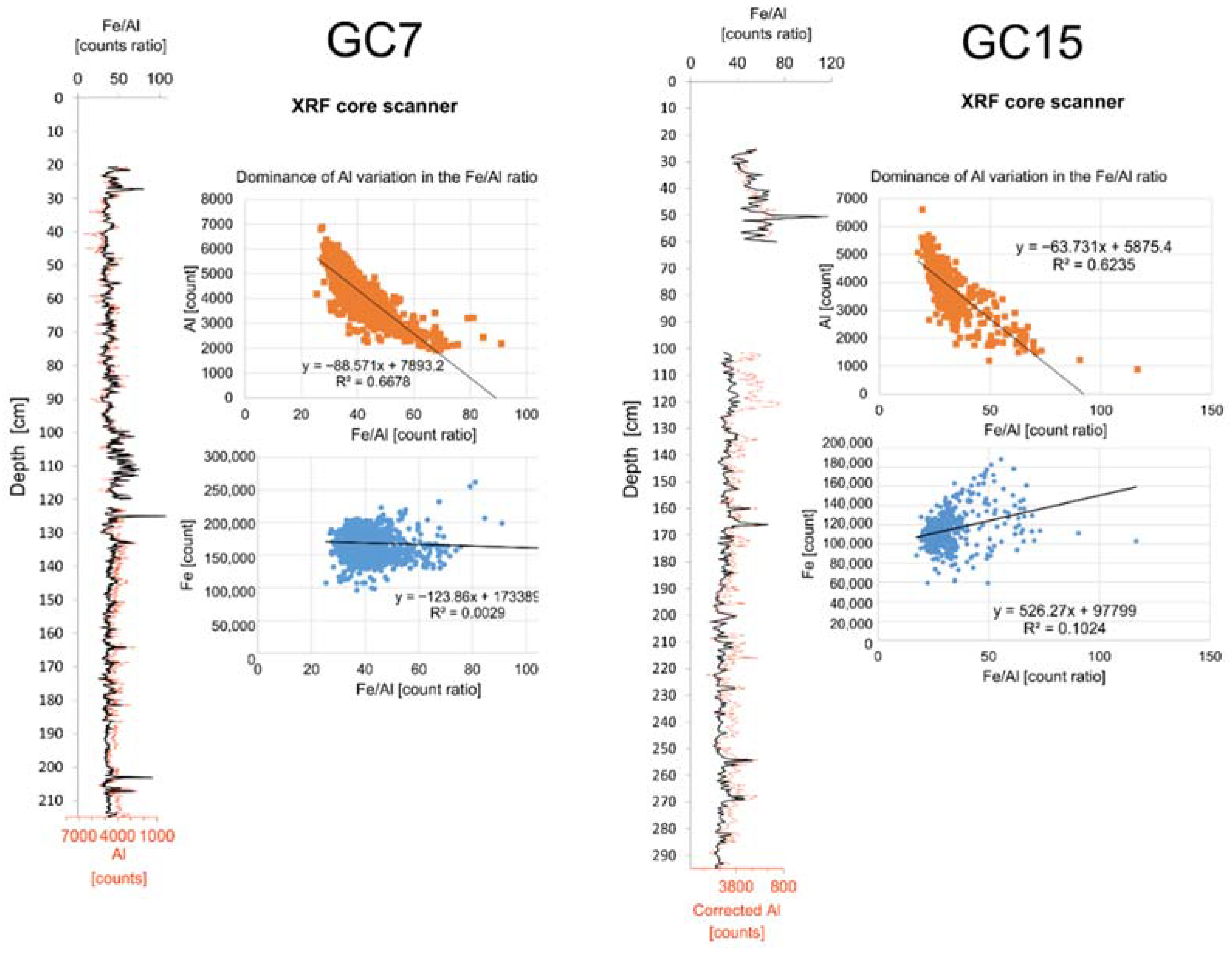
3.5.2. Geochemical Proxies

The organic carbon content and the C/N atomic ratio were measured on decarbonised samples using an elemental analyser (Vario Microcube C-N-S, Elementar Analysen systeme, GMBH, Hanau, Germany) at the Laboratory for Oceanology, University of Liège, Belgium. The upper 97 cm of GC7 were sampled at every cm interval and the upper 60 cm of GC15 at every 2 cm. Some samples were also analysed in the lower part of both cores (

Table A3. Carbon and nitrogen contents and C/N atomic ratio in the GC15 and GC7 cores.

GC15				GC7
Depth [cm]	% N	% C	C/N Atomic Ratio	Depth [cm]	% N	%C	C/N Atomic Ratio
1–5	0.19	2.0	12.3	0–1	0.14	1.5	13.1
5–10	0.20	2.2	13.1	1–2	0.12	1.2	11.7
10–12	0.20	2.2	12.8	2–3	0.13	1.0	9.7
12–14	0.19	2.0	12.2	3–4	0.12	0.9	9.4
14–16	0.21	2.0	11.3	4–5	0.14	1.2	10.0
16–18	0.20	2.1	11.9	5–6.5	0.14	1.3	10.9
18–20	0.22	2.2	11.7	6.5–8	0.12	1.1	11.0
20–22	0.19	2.1	12.6	8–9	0.12	1.0	10.2
22–24	0.20	2.1	12.2	9–10	0.12	1.1	10.4
24–26	0.19	2.2	13.5	10–11	0.13	1.1	9.5
26–28	0.20	2.3	13.7	11–12	0.15	1.2	9.7
28–30	0.21	2.3	12.9	12–13	0.15	1.3	10.3
30–32	0.17	2.2	15.3	13–14	0.14	1.4	11.7
32–34	0.19	2.1	13.2	14–15	0.15	1.3	10.1
34–36	0.21	2.3	12.9	15–16	0.16	1.5	10.7
36–38	0.20	2.2	13.1	16–17	0.14	1.3	10.6
38–40	0.20	1.8	10.3	17–18	0.16	1.6	11.2
40–42	0.23	2.2	11.0	18–19	0.13	1.2	11.1
42–44	0.20	2.0	11.7	19–20	0.14	1.3	10.4
44–46	0.19	1.8	11.0	20–21	0.15	1.7	12.9
46–48	0.18	2.4	15.4	21–22	0.09	0.9	11.7
48–50	0.14	2.5	20.9	22–23	0.14	1.3	11.0
50–52	0.16	2.5	17.6	23–24	0.12	1.0	9.8
52–54	0.18	2.2	14.5	24–25	0.13	1.1	9.8
54–56	0.13	1.9	16.6	25–26	0.12	0.9	9.0
56–58	0.20	2.1	12.3	26–28	0.11	0.8	8.6
104–105	0.13	1.2	9.0	28–29	0.15	1.3	10.5
107–108	0.12	0.9	7.3	29–30	0.14	1.2	10.7
132–133	0.14	1.0	7.3	30–31	0.14	1.2	9.9
151–152	0.06 *	0.5	7.4 *	31–32	0.14	1.2	9.7
167–168	0.07 *	0.5	7.0 *	32–33	0.15	1.1	9.0
175–176	0.07 *	0.5	7.7 *	33–34.5	0.13	1.0	9.2
				34.5–35.5	0.15	1.4	10.9
				35.5–36.5	0.11	1.0	10.3
				36.5–37.5	0.12	1.0	9.3
				37.5–38.5	0.11	0.9	9.8
				38.5–39.5	0.13	1.1	9.3
				39.5–40.5	0.13	1.0	8.9
				40.5–41.5	0.13	1.1	9.7
				41.5–42.5	0.08	0.6	8.8
				42.5–43.5	0.09	0.8	10.8
				43.5–44.5	0.11	0.9	8.8
				44.5–45.5	0.11	0.8	8.3
				45.5–46.5	0.12	1.0	9.5
				46.5–47.5	0.11	0.8	9.2
				47.5–48.5	0.11	0.8	8.2
				48.5–49.5	0.11	0.8	8.0
				49.5–50.5	0.11	0.8	8.7
				50.5–51.5	0.13	1.2	10.2
				51.5–52.5	0.13	1.2	10.0
				52.5–53.5	0.13	1.0	9.5
				53.5–54.5	0.10	1.0	11.2
				54.5–55.5	0.10	0.8	9.2
				55.5–56.5	0.10	0.9	9.6
				56.5–57.5	0.12	1.0	10.1
				57.5–58.5	0.13	1.0	8.8
				58.5–59.5	0.15	1.2	9.6
				59.5–60.5	0.16	1.3	9.3
				60.5–61.5	0.14	1.1	9.3
				61.5–62.5	0.12	1.0	9.7
				62.5–63.5	0.13	0.9	8.5
				63.5–64.5	0.12	1.2	11.6
				64.5–65.5	0.16	1.5	10.7
				65.5–66.5	0.17	1.3	9.3
				66.5–67.5	0.12	0.9	8.9
				67.5–68.5	0.13	1.0	9.3
				68.5–69.5	0.14	1.1	9.7
				69.5–70.5	0.14	1.1	9.1
				70.5–71.5	0.16	1.6	11.9
				71.5–72.5	0.14	1.3	10.6
				72.5–73.5	0.13	1.0	9.0
				73.5–74.5	0.16	1.4	10.1
				74.5–75.5	0.14	1.2	10.2
				75.5–76.5	0.08	0.7	9.3
				76.5–77.5	0.11	1.1	10.9
				77.5–78.5	0.12	1.3	12.1
				78.5–79.5	0.13	1.2	11.0
				79.5–81	0.14	1.2	10.5
				81–82	0.12	1.0	9.8
				82–83	0.13	1.3	11.9
				83–84	0.13	1.1	9.4
				84–85	0.13	1.2	10.6
				85–86	0.13	1.4	12.7
				86–87.5	0.15	1.3	10.4
				87.5–88.5	0.13	1.3	11.5
				88.5–89.5	0.13	1.1	9.9
				89.5–90.5	0.13	1.2	10.3
				90.5–91.5	0.13	1.1	9.4
				91.5–92.5	0.13	0.9	8.7
				92.5–93.5	0.15	1.6	12.3
				93.5–94.5	0.16	1.5	11.1
				94.5–97	0.14	1.3	11.1
				107–108	0.07 *	0.5	7.9 *
				126–127	0.09 *	0.7	7.7 *
				145–146	0.08 *	0.8	10.3 *
				179–180	0.10 *	0.8	8.2 *

* low N content leading to a less reliable C/N value.

).

X-ray fluorescence (XRF) core scanner measurements were performed by the EPOC Laboratory (University of Bordeaux, France). The sediment in the plastic sleeves was covered by a 4 µm ultralene film before being scanned at high resolution by an AVAATECH XRF core scanner (third generation, rhodium X-ray tube, silicon detector X PIPS–Canberra). Relatively light elements (e.g., Al, Ti and Fe) were detected with a scan at 10 kV (2000 µA and 20 s for GC7, 1000 µA and 10 s for GC15). The applied correction was the division, at each depth, of the number of counts of a specific element by the sum of counts for all elements analysed at that depth, then multiplied by the average sum:

$$\mathrm{corrected} \mathrm{counts}=\frac{\mathrm{counts}}{{{\displaystyle \sum }}^{ }\mathrm{counts} \mathrm{for} \mathrm{all} \mathrm{elements}}\times \overline{{{\displaystyle \sum }}^{ }\mathrm{counts} \mathrm{for} \mathrm{all} \mathrm{elements}}$$

(4)

The advantages of the XRF core scanner are the continuity and the high resolution of data (1 mm for GC7 and 5 mm for GC15). We tested two hypotheses on our XRF data:

• It should be possible to distinguish Fe with a detrital signature from Fe remobilised due to changes in redox conditions;
• High Fe/Al ratio in our cores could be used as a proxy for anoxia as in Spofforth et al. [26].

To challenge the first hypothesis, principal component analyses (PCA) were performed on XRF core scanner data using the R software (PCA function in the FactoMineR library). We considered that Fe has a detrital signature if it is correlated with Al, Si, K and Ti while, if there is no correlation, we assumed that Fe was remobilised after its initial deposition due to changes in redox conditions.

For the second hypothesis, we investigated the meaning of Fe/Al variations in the high-resolution XRF core scanner data. Al is a light element with a high coefficient of variation in the data compared to Fe. Therefore, the Fe/Al ratio was dominated by the noisy variations of Al in both cores (see Figure A1). PCA analysis and visual inspection showed that changes in Si, K, Ti and Al were close, but Al was the noisiest element. In our case, it was better to use Ti as a denominator to investigate the usefulness of the Fe/Ti ratio as a proxy. A set of samples were taken at the position of Fe/Ti peaks in order to test the consistency with another proxy, i.e., the framboidal pyrite observations.

Bulk elemental analyses were performed on 100 mg of dry sub-sample from 1 cm thick sediment slices at the Geochemical Laboratory of the Central Africa Royal Museum, Brussels, Belgium. Several elements (e.g., Al, S) were measured with a Thermo Iris Advantage Inductively Coupled Plasma–Optical Emission Spectrometry (ICP-OES, 14 samples from GC7 and 8 from GC15). Inductively coupled plasma–mass spectrometry (ICP-MS) analyses were carried out with a Thermo Fisher Scientific X-Series2 ICP-MS (28 samples from GC7 and 17 from GC15) to measure several redox-sensitive elements (e.g., V, Fe, U). The low range of elemental variations measured by ICP-OES and ICP-MS did not allow the calibration of XRF core scanner data.

Laser ablation (LA-ICP-MS) was used on 3 resin-embedded blocks (high-resolution data over 1 cm) to determine the Mo concentration. Mo was measured on three samples representative of: (1) the whole GC7 (no framboidal pyrites), (2) levels in GC15 showing large framboidal pyrites and (3) levels in GC15 containing small framboidal pyrites (see hereafter for interpretation of framboidal pyrite proxy).

For V, U and Mo, enrichment factors (EF) were calculated with respect to the average upper crust composition [36]:

$$\mathrm{EF}=\frac{{\left(\raisebox{1ex}{$\mathrm{X}$}\!\left/ \!\raisebox{-1ex}{$\mathrm{Al}$}\right.\right)}_{\mathrm{sample}}}{{\left(\raisebox{1ex}{$\mathrm{X}$}\!\left/ \!\raisebox{-1ex}{$\mathrm{Al}$}\right.\right)}_{\mathrm{upper} \mathrm{crust}}}$$

(5)

Iron sequential extraction was carried out to determine the reactive iron speciation using the method of Kraal et al. [27] modified from Claff et al. [37] in 11 samples from GC7 and 15 samples from GC15. Four iron fractions were separated: Fe_H (easily extractable fraction with labile ferrous, i.e., FeS and siderite, and ferric iron, i.e., ferrihydrite, akaganeite and lepidocrocite), Fe_org (iron bound to organic matter), Fe_ox (hematite and goethite) and Fe_pyr (pyrite). The different fractions were analysed by atomic absorption (Analytik Jena AA400 model, University of Liège). Reactive iron (Fe_reactive) was calculated as:

Fe_reactive = Fe_H + Fe_org + Fe_ox + Fe_pyr

(6)

3.5.3. Mineralogical Proxy: Framboidal Pyrites

Pyrite was first detected using X-ray diffraction (XRD). XRD analyses were carried out every 5 cm on powdered samples (44 for GC7 and 27 for GC15) using a Bruker D8 Advance Eco (Cu X-ray tube, Kα = 1.54 Å, scan between 2° and 70° 2θ, LinxEye XE detector) at the University of Liege (Mineralogy and Crystallography Laboratory and Clay, Geochemical and Sedimentary Environments Laboratory). Diffractograms were analysed with the EVA v.3.2. software (Bruker AXS GmbH) and the Crystallography open database.

Framboidal pyrites of 8 samples from GC7 and 15 samples from GC15 were observed with an SEM (ESEM-FEG XL30 model, at 15 kV, with a working distance of 10 mm) at the University of Liège. Moreover, samples from the top 4 cm (samples from 0–2 and 2–4 cm depths) of the multicorers MC7 and MC15 were observed to investigate the most recent sediments. Samples were sieved at 63 µm. The clay fraction (<2 µm) was removed by successive centrifugations (8 × 8 min at 700 rounds per minute). The fraction between 2 and 63 µm was conserved and coated with carbon to allow the detection of framboidal pyrites with the back-scattered electron (BSE) mode. In the BSE mode, pyrite seemed brighter than the surrounding minerals due to its relatively higher atomic number [38]. Energy-dispersive X-ray spectrometry (EDS) analysis confirmed the identification of framboidal pyrites when needed. Generally, a minimum of 100 diameters are measured per sample in studies using this proxy [19,20]. In this work, 30 diameters per sample, i.e., the minimum statistically recommended [39], were measured at 3000×magnification. The mean between two measured diameters per pyrite was calculated.

4. Results

4.1. Benthic Foraminifera

The number of individuals observed varied between the two cores depending on the depth. Few individuals were found in the different granulometric fractions (>63 µm, >150 µm, >250 µm) of GC7 (Figure 6B). On the contrary, for the GC15 core, several hundreds to thousands of individuals were observed (Figure 7B). The most abundant genus found in GC7 and GC15 is the genus Ammonia (Figure 4D). It accounts for more than 93% of the counted foraminifera. The genus Elphidium (Figure 4 E,F) constitutes 0.5 and 1.8% of the individuals, respectively, for GC7 and GC15 (0–1 individual in GC7 and 0–11 in GC15; Figure 6B and Figure 7B;

Table A4. Number of Ammonia, Elphidium and Nonion foraminifera counted in GC7 and GC15 samples with the calculated values of the A-E index (for the fraction > 150 µm). Total foraminifera includes non-identified individuals (minor genus or badly preserved).

		Number of Foraminifera
Core	Depth (cm)	Ammonia NA	Elphidium NE	Nonion	Total	A-E Index (NA/(NA + NE)) × 100
GC7	28–29	12	1	0	17	92
	43.5–44.5	6	0	0	9	100
	101–102	59	1	0	66	98
	112–113	25	0	1	29	100
	126–127	13	0	0	13	100
	133–134	32	0	1	36	100
	134–135	31	0	0	37	100
	151–152	49	0	0	49	100
	163–164	198	1	0	200	99
	165–166	6	0	0	6	100
	179–180	57	0	1	58	100
	204–205	6	0	0	6	100
GC15	42–44	184	3	11	199	98
	50–52	170	11	19	200	94
	134–135	193	4	3	200	98
	147–148	147	0	1	151	100
	163–164	58	1	1	60	98
	165–166	182	3	14	200	98
	167–168	189	0	5	194	100
	187–188	190	3	7	200	98

). The remaining percentage of individuals corresponds to genus Nonion or to other minor unidentified genera0 (Table A4). The computed A-E index varies between 92 and 100% for GC7 and between 94 and 100% for GC15 (Table A4).

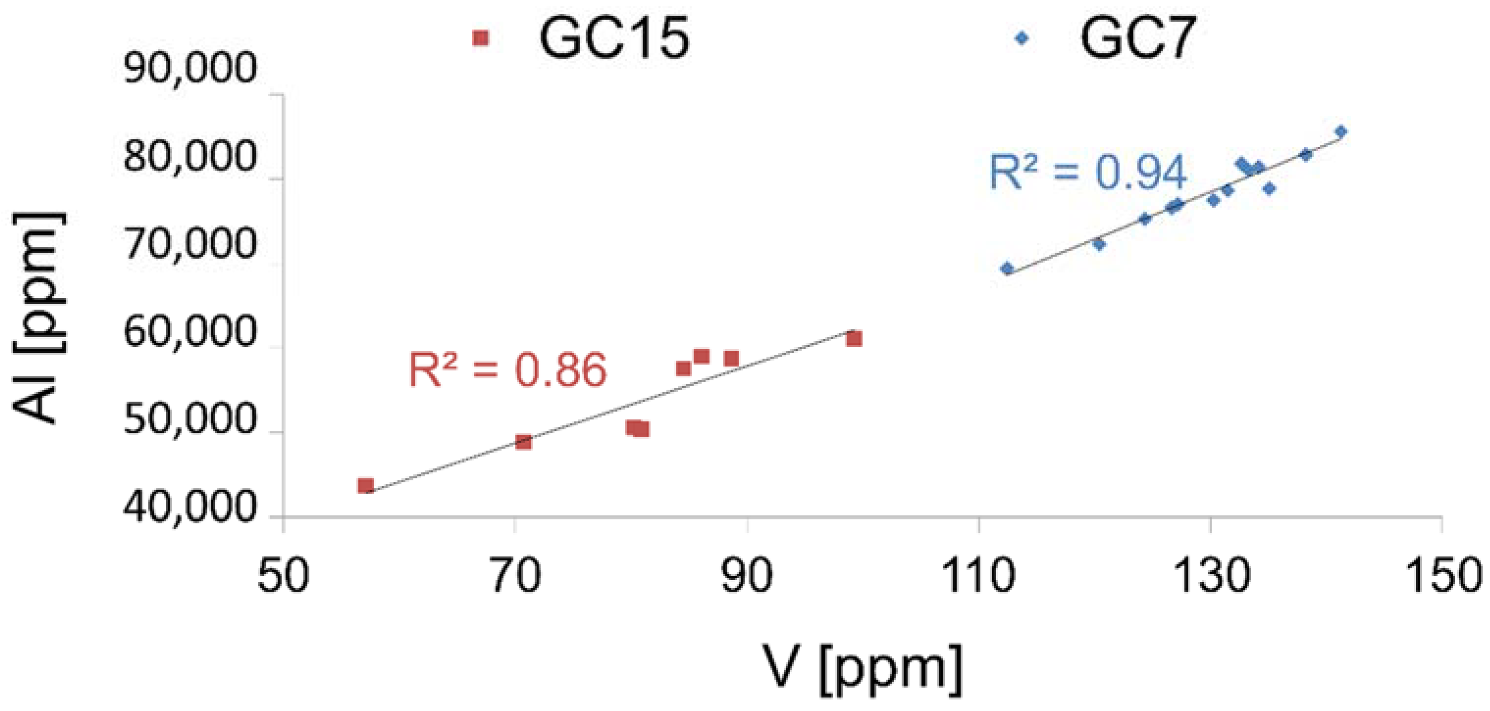
4.2. Geochemical Proxies

C_org and C/N atomic ratio data are reported in Table A3. The mean organic carbon content was slightly lower in GC7 (1.1 wt %) than in GC15 (1.9 wt %). The C_org content (Figure 6C for GC7 and Figure 7C for GC15) and the C/N ratio (Figure 6D for GC7 and Figure 7D for GC15) decreased with depth in both cores. For GC7, the mean % C_org was 1.1 wt % and the mean C/N atomic ratio was 10.1 in the top 97 cm. In the bottom part of the core, the mean % C_org was 0.7 wt % and the mean C/N ratio was 8.5 (note the low number of data). For GC15, in the upper 60 cm, the mean % C_org was 2.1 wt % and the mean C/N atomic ratio was 13.3, with a peak of 20.9 indicating a terrestrial organic matter input [40]. Below Unit 3, the % C_org (0.8 wt %) and C/N (7.6) were lower.

Three trace metals were targeted: V, U and Mo (

Table 2. Average trace metal concentrations in GC7 and GC15 and corresponding enrichment factors calculated with respect to the average upper crust abundance [36].

Element	Average Upper Crust Abundance [ppm]	GC7		GC15
		Concentration [ppm]	Enrichment Factor	Concentration [ppm]		Enrichment Factor
V a	107	130 ± 8	1.3	80 ± 10		1.1
U a	2.8	2.7 ± 0.1	1.0	2.9 ± 0.2		1.5
Mo	1.5	0.86 b,1	0.6	0.96 b,2	1.12 b,3	1.0	1.1
Al c	80,400	78,312	/	53,726		/

^a Average of ICP-MS measurements on 28 samples for GC7 and 17 samples for GC15 (samples of 1 cm thick). ^b Average over 1 cm of high-resolution LA-ICP-MS measurements on (1) an “oxic” sample from GC7 (no framboidal pyrites); (2) a “dysoxic” sample from GC15 (big framboids) and (3) an “anoxic” sample from GC15 (small framboids, 163–164 cm depth). ^c Average of ICP-OES measurements on 14 samples for GC7 and 8 samples for GC15 (samples of 1 cm thick).

). First, the correlation between these trace elements and Al was tested to check if the trace element behaviour was controlled by the detrital inputs, as shown in Tribovillard et al. [18]. V was highly correlated with Al with R² = 0.94 in GC7 and R² = 0.86 for GC15 (Figure A2), contrary to U and Mo. Thus, V could not be used as an anoxia proxy in our case study. There was a slight enrichment in U in GC15 (EF = 1.5, Table 2). Mo concentration was low in the three representative samples and presented no enrichment (Table 2).

The correlation between iron and detrital elements was investigated using principal component analysis (PCA) on XRF core scanner data. In GC7 (Figure 8A), and in the bottom part of GC15 (Figure 8C), Fe was not correlated with any detrital elements (i.e., Al, Si, K, Ti); it was rather correlated with S. In the upper part of GC15 (Figure 8B), iron was closer to the detrital element cluster. These results suggest a modification of the iron behaviour with depth in GC15 (Figure 8B,C).

The continuous semi-quantitative Fe counts in the XRF core scanner (Figure 6F and Figure 7F) were plotted together with ICP-MS quantitative Fe concentrations (Figure 6G and Figure 8G). It illustrates the absence of possible calibration between the two methods. Moreover, the variations in Fe/Ti measured with the XRF core scanner are displayed in (Figure 6H and Figure 7H.

Reactive iron, i.e., the sum of all the extracted fractions represents, on average, 36 ± 4% of total iron in GC7 and 38 ± 6% in GC15. In GC15, reactive iron accounted for 32 to 55% of the total iron (

Table A5. Reactive iron speciation (Fe_reactive) for the GC15 and GC7 cores. Fe_H (easily extractable fraction with labile ferrous, i.e., FeS and siderite, and ferric iron, i.e., ferrihydrite, akaganeite and lepidocrocite), Fe_org (iron bound to organic matter), Fe_ox (hematite and goethite) and Fe_pyr (pyrite).

GC15						GC7
Depth	Fereactive	FeH	Feorg	Feox	Fepyr	Depth	Fereactive	FeH	Feorg	Feox	Fepyr
[cm]	[% of Fetotal]	[% of Fereactive]				[cm]	[% of Fetotal]	[% of Fereactive]
14–16	32	46	9	25	20	28–29	41	86	7	1	7
18–20	34	47	9	21	23	43.5–44.5	*	79	10	1	9
24–26	38	44	8	18	30	101–102	*	85	6	1	7
28–30	33	50	6	5	39	107–108	34	83	9	2	6
34–36	37	45	7	5	44	113–114	33	87	6	1	6
40–42	36	55	8	4	33	126–127	*	89	5	1	5
50–52	*	39	6	2	53	133–134	*	91	4	1	4
56–58	55	36	5	3	56	145–146	*	91	4	1	4
104–105	41	10	8	4	79	151–152	*	90	4	1	4
107–108	38	7	10	4	79	179–180	*	86	6	2	7
132–133	36	10	8	4	78	204–205	*	91	5	1	3
151–152	32	8	9	4	80	Mean ± SD	36 ± 4	87 ± 4	6 ± 2	1 ± 0.4	6 ± 2
163–164	*	26	8	2	65
167–168	37	8	8	3	81
175–176	39	6	10	3	81
Mean ± SD	38 ± 6	26 ± 19	8 ± 1	5 ± 8	61 ± 23

* Total iron not measured.

). In both cores, Fe_org was not abundant and remained relatively constant (5 to 10% of reactive iron; Table A5). In GC7, the reactive iron speciation was homogeneous (Figure 6I), dominated by the Fe_H fraction (87 ± 4% of reactive iron). The other fractions were less abundant. The pyrite fraction only corresponded to 6 ± 2% of reactive iron (Table A5). In contrast, GC15 showed an iron reduction with depth (Figure 7I). Indeed, the Fe_pyr fraction gradually increased with depth from 20% up to 80% of reactive iron at the expense of the Fe_ox and Fe_H fractions (Figure 7I).

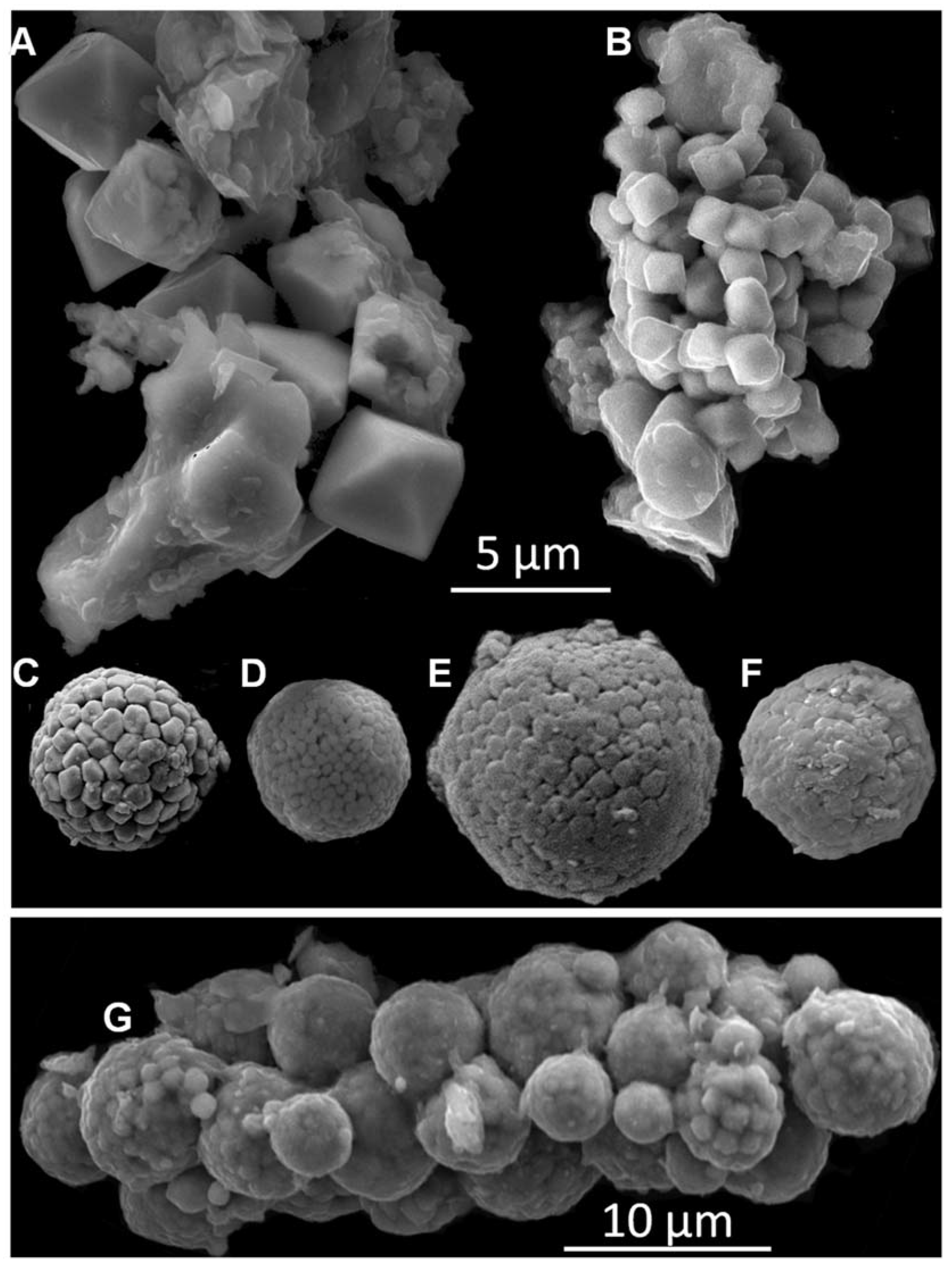
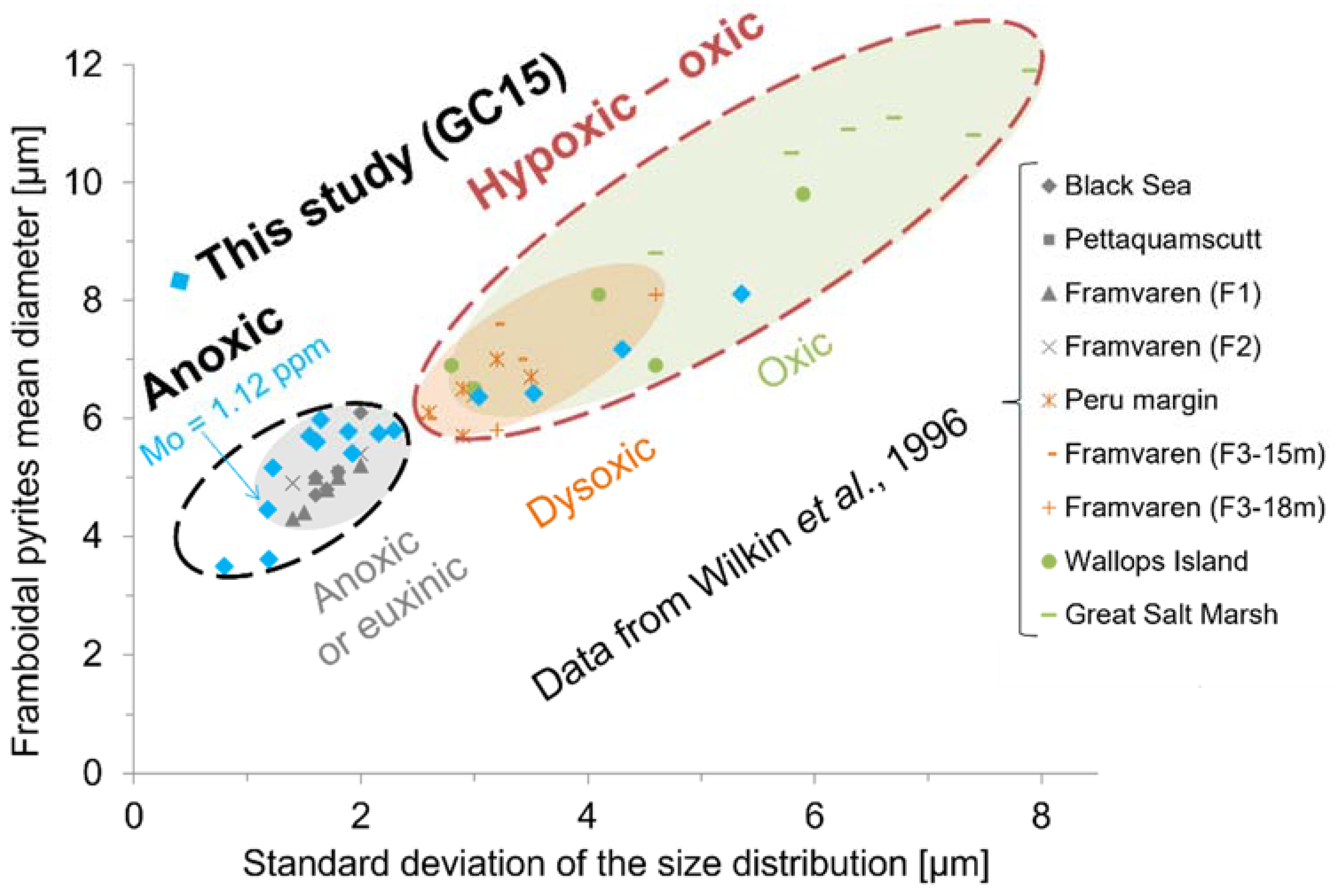
4.3. Mineralogical Proxy: Framboidal Pyrites

Pyrite is composed of iron and sulphur. Total Fe content, measured by ICP-MS, varied between 3.8 ± 0.2 and 5.2 ± 0.2 wt % for GC7 (Figure 6G) and between 2.1 ± 0.1 and 4.4 ± 0.2 wt % for GC15 (Figure 7G). Thus, total iron was, on average, more abundant in GC7 (4.5 ± 0.3 wt %) than in GC15 (3.1 ± 0.6 wt %). However, total iron could not be used directly as a proxy because it indicates neither the iron redox-state nor the amount of pyrite. Sulphur, measured by ICP-OES, was, on average, less abundant in GC7 (0.26 ± 0.20 wt %, Figure 6E) than in GC15 (1.21 ± 0.51 wt %, Figure 7E).

In GC7 (Figure 6J), no framboidal pyrites were found in the samples observed with the SEM, which was consistent with the absence of pyrite detected by XRD and the low amount of Fe_pyr extracted. The absence of pyrite was also noticed in the uppermost samples collected close to the water-sediment interface in MC7 (Figure 6J).

In GC15, the detection of pyrite by XRD and by sequential extraction (61 ± 31% of reactive iron) was confirmed by SEM observations of framboids (Figure 4G,H). The size distributions of the 30 diameters measured per sample (Figure 7J,

Table A6. Size distribution of the diameters of framboidal pyrites in 15 samples from GC15 (30 diameters) and one sample from MC15 (8 diameters).

Depth	Number of Framboidal Pyrites per Classes of Diameters Measured in µm																					Mean Diameter ± SD
[cm]	[1, 2[	[2, 3[	[3, 4[	[4, 5[	[5, 6[	[6, 7[	[7, 8[	[8, 9[	[9, 10[	[10, 11[	[11, 12[	[12, 13[	[13, 14[	[14, 15[	[15, 16[	[16, 17[	[17, 18[	[18, 19[	[19, 20[	[20, 21[	[21, 22[	[µm]
1–5	1	2	3	6	8	4	4	/	2	/	/	/	/	/	/	/	/	/	/	/	/	5.4 ± 1.9
10–12	/	3	7	/	6	8	1	2	2	/	1	/	/	/	/	/	/	/	/	/	/	5.8 ± 2.3
18–20	1	1	5	4	7	5	1	4	/	2	/	/	/	/	/	/	/	/	/	/	/	5.7 ± 2.2
28–30	/	1	1	6	5	7	2	2	1	/	/	/	/	1	/	/	/	/	2	1	1	8.1 ± 5.4
40–42	/	/	3	4	13	3	3	3	1	/	/	/	/	/	/	/	/	/	/	/	/	6.0 ± 1.6
50–52	/	/	3	9	7	5	3	2	/	1	/	/	/	/	/	/	/	/	/	/	/	5.6 ± 1.6
104–105	1	7	14	7	1	/	/	/	/	/	/	/	/	/	/	/	/	/	/	/	/	3.5 ± 0.8
132–133	2	8	12	4	3	/	1	/	/	/	/	/	/	/	/	/	/	/	/	/	/	3.6 ± 1.2
141–142	/	1	6	4	6	3	3	3	1	/	1	/	/	2	/	/	/	/	/	/	/	6.4 ± 3.0
151–152	/	1	5	2	7	5	2	2	1	1	1	/	/	1	/	/	/	1	/	/	1	7.2 ± 4.3
163–164	/	3	8	11	5	2	1	/	/	/	/	/	/	/	/	/	/	/	/	/	/	4.5 ± 1.2
175–176	/	3	2	4	16	3	2	/	/	/	/	/	/	/	/	/	/	/	/	/	/	5.2 ± 1.2
186–187	/	/	4	5	12	4	2	/	/	/	/	/	/	/	1	2	/	/	/	/	/	6.4 ± 3.5
196–197	/	2	3	5	6	6	4	3	/	1	/	/	/	/	/	/	/	/	/	/	/	5.8 ± 1.9
268–269	/	1	1	7	12	6	/	2	/	1	/	/	/	/	/	/	/	/	/	/	/	5.7 ± 1.5
MC15: 2–4	/	/	1	1	1	/	/	2	1	1	/	/	/	/	/	/	/	/	/	/	/	not enough data

) could be divided into two groups. The “small” group included samples with a mean framboid diameter ranging between 3 and 6 µm with a narrow standard deviation (1 or 2 µm), while the “big” group included samples with a mean framboid diameter varying between 6 and 10 µm with a wider standard deviation (3 to 5 µm). In MC15 (Figure 7J), the sample just below the water-sediment interface (0–2 cm) showed no framboidal pyrites. The 2 to 4 cm sample contained rare framboidal pyrites, preventing any calculation of a robust mean.

5. Discussion

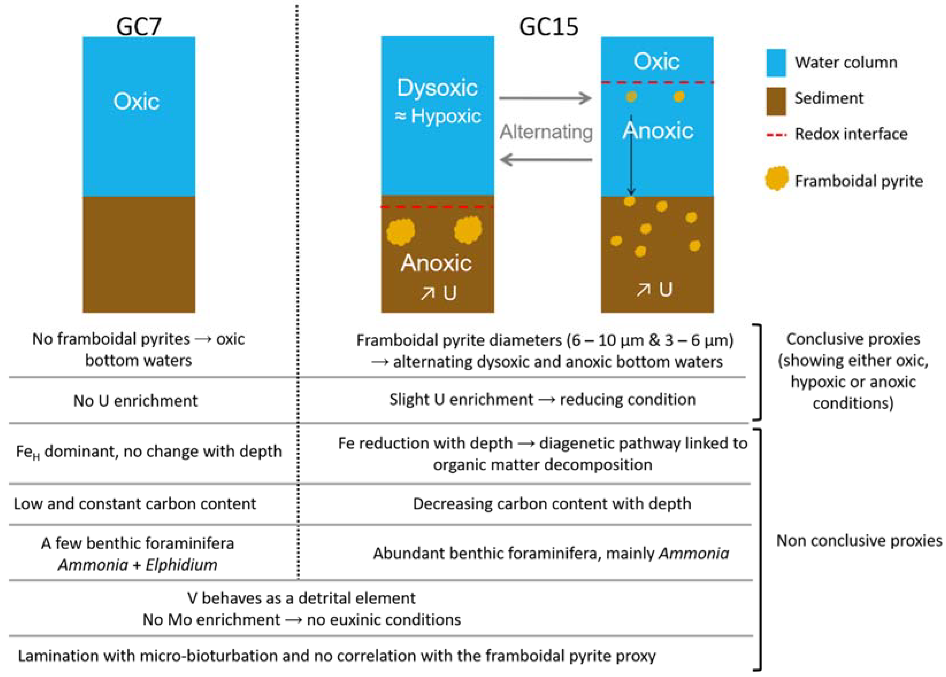
5.1. Past Oxygenation of the NW Black Sea Shelf Inferred from the Framboidal Pyrite Proxy

Among all proxies tested in this study, only the presence of framboidal pyrites and their characteristics (i.e., mean diameter and its standard deviation) were directly connected with the level of oxygenation of bottom waters. Up to now, all studies using framboidal pyrites as a proxy were based on the pioneering research of Wilkin et al. [19], who linked the size of framboidal pyrites in modern sediments with the oxygen level of bottom waters in various oxygenated basins. The GC15 results are reported in parallel with the observations of Wilkin et al. [19], where the mean framboid diameters are plotted against the standard deviations of the size distributions (Figure 9). Two categories of oxygenations can be inferred from this graph.

First, the current anoxic-euxinic basins show small framboid diameters and narrow standard deviations [19]. Eleven of the GC15 samples fell in the field of anoxic-euxinic conditions (Figure 9). In a sample considered as representative of the small framboids group in GC15, the absence of Mo enrichment rules out euxinic conditions, according to Tribovillard et al. [18]. In Figure 9, we define an “anoxic” field around the GC15 results with small mean diameters, including the two samples from GC15 representing the smallest mean diameters.

Second, dysoxic and oxic modern basins produce framboids with larger diameters and wider standard deviations [19]. The fields of dysoxic and oxic conditions are superimposed in Figure 9, even if the oxic field is elongated towards a larger diameter and wider standard deviation. Therefore, it is not possible to distinguish dysoxic environments from oxic ones with only the framboidal pyrite measurements. In Figure 9, we regroup the dysoxic and oxic fields into one field called the “hypoxic-oxic” field, represented by a dashed red ellipse; four samples from GC15 fall into that field.

No correlation can be highlighted between the lithological changes in GC15 and the oxygenation variations deduced from framboidal pyrites. Indeed, Figure 7J shows that Units 1, 6 and 8 contain framboidal pyrites belonging to the “small” group (i.e., “anoxic” conditions) as well as to the “big” group (i.e., “hypoxic-oxic” conditions). All the samples from Units 2, 4, 7 and 9 belong to the “small” group (Figure 7J), suggesting anoxic bottom waters, but new samples could reveal framboidal pyrites belonging to the “big” group or no framboids at all. Four of the GC15 samples fall in the “hypoxic-oxic” field, while 11 samples fall in the “anoxic” field (Figure 9). Consequently, the Odessa Bay (GC15 location) underwent an alternation between anoxic and hypoxic to oxic conditions during the past 7.4 ka. The absence or the rarity of framboidal pyrites in the top sediment of MC15 suggests that the current conditions in the Odessa Bay are not favourable for the formation of framboidal pyrites due to a high oxygen level during one part of the year on the shelf or to other controlling factors.

In GC7, the absence of framboidal pyrites can be interpreted as an indication of an oxic water column during sediment deposition, according to the classification of Bond and Wignall [20] (Figure 1). However, Wilkin et al. [19] found framboidal pyrites in modern oxic basins (Figure 9). This contradiction suggests that the oxygenation level is not the only factor controlling the framboid formation. The absence of pyrite in GC7 might be linked to the lower amount of sulphur in this core compared to GC15 (Figure 6E and Figure 7E). Future studies on the sulphur speciation of the GC7 and GC15 cores should allow the determination of the proportion of sulphur associated with pyrite (e.g., [41]). The observation of the top sediment of MC7 indicates that there is currently no framboidal pyrite formation in front of the Danube mouth.

The sample preparation in this study (i.e., loose sediment, only the fraction between 2 and 63 µm) does not allow us to estimate the abundance/density of framboidal pyrites, which is one of the criteria used in the classification of past oxygen levels defined by Bond and Wignall [20]. Thus, it could be interesting to evaluate the abundance of framboidal pyrites. Moreover, several pyrite morphologies were encountered in the GC15 core: euhedral crystals, loose aggregates of microcrystals, framboidal pyrites (totally, partially or not at all filled-in by pyrite secondary growth) and a cluster of framboidal pyrites (Figure A3). It could also be relevant to systematically report the pyrite morphologies as they may provide some clues about the formation environment.

5.2. Other Proxies Considered as Inappropriate in the Case of the Black Sea Coastal Environment

In our case study of the Black Sea coastal environment, other proxies are not as conclusive as the framboidal pyrite proxy concerning the bottom water oxygenation (Figure 10).

5.2.1. Laminations

The use of the laminated intervals was not relevant in our case to detect hypoxia, but it might be in other cases (as used in the Baltic Sea by Zillén et al. [15]). Indeed, several units of GC7 and GC15 are macroscopically laminated, but bioturbated in thin sections. Moreover, oxic conditions are suggested in both laminated and non-laminated intervals of GC7 (Figure 6A,J). Similarly, there was no relation between the lamination of the sediment in GC15 (Figure 7A) and the occurrence of framboidal pyrites, whatever their size (Figure 7J). Moreover, anoxia was suggested by the small framboidal pyrites observed in U1 and U9 of GC15, and both units were not laminated.

5.2.2. Foraminifera

According to Sen Gupta et al. [16], when the A-E index is close to 100% (i.e., when the genus Ammonia is over-represented in the assemblages compared to the genus Elphidium), it suggests a hypoxic environment. This was the case in both GC7 and GC15, with an A-E index between 92 and 100%. In GC7, the results were questionable: the number of observed individuals rarely reached 200, and for all analysed samples, either one or no Elphidium were identified (Figure 6B; Table A4). Thus, computing this index for GC7 seems to be unreasonable.

As highlighted by Sen Gupta and Platon [42], this index can only be used under strict conditions: high sedimentation rate, water depth less than 30 m, minimally bioturbated sediments and constant salinity. Observations of the thin sections and of the SCOPIX (Figure 3) have shown, respectively, that the sediment is bioturbated and reworked in GC7 and GC15, which may contribute to the erroneous results of the index. Additionally, the average salinity and its variations have a strong impact on the index [42]. This parameter influences the diversity in the assemblage of foraminifera, and a local decrease in salinity on the Black Sea shelf can trigger an impoverishment of the assemblage [22]. At the coring locations, in a proximal environment and next to the mouth of rivers, the average salinity was low, and the fluctuations of salinity were important. The abundance of Ammonia spp. and the near absence of Elphidium spp. may be due to the higher resistance of the genus Ammonia living in mesohaline and polyhaline waters [14], to the decrease of salinity and not necessarily to the lack of oxygen. Moreover, the average salinity (only a few ‰) at the coring location of GC7, i.e., at the mouth of the Danube, may explain the low number of individuals observed in the samples [22]. This relationship between the salinity and the abundance of Elphidium was demonstrated by Cronin et al. [43], who used the Elphidium genus to reconstruct the variability of the salinity during the last centuries in the Chesapeake Bay (USA). The authors highlighted that the higher the salinity, the higher the abundance of Elphidium in the foraminiferal assemblages. Few or no Elphidium individuals are found at salinity values ≤ 10‰ (closer to the coast).

Parameters other than oxygen concentration and salinity also influence the benthic foraminifera and their assemblages, such as the substrate, temperature, luminosity and nutrient availability [44]. Thus, all these coastal parameters must be considered when interpreting the results of the A-E index. We cannot, therefore, conclude if this index could be used to identify hypoxic events that occurred on the NW Black Sea shelf during the Holocene.

To determine if the A-E index is applicable in the context of the Black Sea shelf, it would be more relevant to take sediment at a greater distance from the mouth of the rivers. This may allow clear documentation of the hypoxic signal in the sediment without the influence of the salinity and its variations. It is also possible that the much lower average salinity of the Black Sea (~17‰), compared to the optimal salinity (~35‰) [44] for most of the foraminifera, renders the use of this index complicated.

5.2.3. Organic Matter

In both cores, C_org content decreased with depth. No significant enrichments in organic matter have been measured (max 1.7 wt % for GC7 and max 2.5 wt % for GC15) as compared to the 5 to 10 wt % (up to 15 wt %) recorded in the Baltic Sea during hypoxic periods [23,24,25]. Thus, we cannot identify short episodes of oxygen restriction on the Black Sea shelf. However, there was slightly more organic carbon in GC15, where the presence of framboidal pyrites suggests oxygen depletion, as compared to GC7, where oxic conditions are assumed.

The C/N atomic ratios indicate, according to the range of values presented in Leng and Lewis [40], the dominance of organic matter with a marine or freshwater origin (C/N < 12), except for the peak value observed in GC15, which suggests an input of terrestrial plants (C/N > 12).

5.2.4. Trace Metals

Results of trace metals were not conclusive. V behaves mainly as a detrital element and cannot be used as a hypoxia proxy. U was slightly enriched in GC15, suggesting reducing conditions, which is consistent with the framboidal pyrite proxy. U was not enriched in GC7, suggesting conditions different from GC15. Low Mo contents indicate that euxinic conditions are unlikely.

Table 3. Trace metal concentration in three embedded blocks analysed by LA-ICP-MS representative of 3 different oxygenation conditions in bottom waters.

Core	Depth (cm)	Framboidal Pyrites	Oxygenation Level Inferred	Average Concentration (maximum) ppm
				V	U	Mo
GC7	106.5–107.6	none	oxic	105 (179)	2.0 (30.5)	0.86 (10.67)
GC15	151–151.8	big group	hypoxic/oxic	91 (199)	2.7 (45.8)	0.96 (6.73)
GC15	162–164.2	small group	anoxic	104 (165)	3.0 (57.7)	1.12 (11.28)

shows that trace metal concentrations (V, U and Mo) were relatively similar in the intervals considered as representative of: (1) oxic conditions in GC7, (2) hypoxic/oxic conditions in GC15 and (3) anoxic conditions based on the framboidal pyrite proxy. Future research with additional measurements should confirm these findings.

5.2.5. Iron Behaviour

In our study, the total iron concentration, as well as Fe/Ti ratio, was not useful for estimating the past oxygenation. The anoxic/hypoxic periods suggested by punctual high Fe/Ti values could not be further validated by the framboidal pyrite observations. Indeed, in GC7, some peaks of Fe/Ti appeared, but no framboidal pyrites were found at the corresponding depths, suggesting oxic conditions. In GC15, at depths where framboidal pyrites were observed, peaks of Fe/Ti and S/Ti were not always present.

Moreover, XRF semi-quantitative data should be used with caution because the counts depend not only on the atomic number of the element but also on many factors, such as water and organic matter contents, grain size and surface irregularities [45]. Furthermore, the low range of elemental variations measured by ICP-MS and ICP-OES did not allow us to calibrate the XRF core scanner data. Consequently, the XRF core scanner data did not seem to be reliable enough to allow the detection of anoxia/hypoxia in this study.

A change in the iron behaviour between the upper and bottom parts of GC15 was suggested by PCA. This is consistent with the occurrence of iron reduction with depth detected by the iron speciation. This iron reduction was linked to the decomposition of organic matter within the sediment during diagenesis [17]. However, it provided no clear indication regarding the water column oxygenation.

Concerning iron speciation, the sequential extraction process of Poulton and Canfield [46] should be used in further research. Following this procedure, the bottom waters of the deposition environment are considered anoxic [47] if the ratio between reactive Fe and total Fe is greater than 0.38. The bottom waters are regarded as euxinic [48] if the ratio between pyrite iron and reactive iron is greater than 0.8. van Helmond et al. [49] successfully used these ratios to conclude that a coastal location in the Baltic Sea underwent anoxia and not euxinia during the Holocene. However, we could not use these ratios in our study because the reactive iron determined following Kraal et al. [27] (see Equation (6)) is not exactly the same as that assessed according to Poulton and Canfield [46].

6. Conclusions

This work, based on the study of two sedimentary cores, highlighted that the Danube mouth (GC7 location) and the Odessa Bay (GC15 location) underwent different oxygenation conditions over the time period covered by the sedimentary record.

Our results demonstrate that the most common biological and geochemical proxies of hypoxia proposed in the literature are irrelevant for the case study of the Black Sea coastal environment. For instance, the Ammonia-Elphidium index appears to be unsuitable for the NW Black Sea shelf, mainly in the case of the Danube mouth (GC7), where only a few foraminifera individuals have been found in the sediments. We assume that the foraminiferal assemblages are salinity-biased due to the influence of freshwater inputs, which decreases the salinity at both sites. We advise using this proxy far from the river mouths to reduce the influence of the salinity on foraminiferal assemblages. Likely, the redox-sensitivity of elements such as vanadium is obscured by the dominant supply of detrital elements in proximal environments.

However, a proxy for hypoxia derived from the size distribution of sedimentary framboidal pyrites provides clear indications of the oxygenation state of the water column. Indeed, the absence of framboidal pyrites in the core located near the Danube mouth (GC7) suggests permanent oxic conditions at least over the last ~1750 years. This is in agreement with the low pyrite iron content (6 ± 2% of reactive iron) measured by sequential extraction. On the contrary, a downward increase in pyrite iron content (from 20% up to 80% of reactive iron) was observed in the other core (GC15). In addition, the two size ranges of framboidal pyrites measured in this core evidence that bottom waters experienced alternating oxic/dysoxic (mean pyrite diameter 6–10 ± 3–5 µm) and anoxic (mean pyrite diameter 3–6 ± 1–2 µm) conditions during the last ~7400 years. These reducing conditions are supported by the slight enrichment in U of the sediment. Euxinic conditions were unlikely given that no Mo enrichment was measured.

Thus, the framboidal pyrite proxy revealed different oxygenation conditions over the Holocene for the two sites investigated. Moreover, our study confirms that the size of framboidal pyrites observed in the NW Black Sea coastal sediments can be used as a proxy to detect hypoxia or anoxia even in a proximal environment.

As stated by Rickard [39], new data are required for recent sediments collected from basins exhibiting various degrees of oxygenation in order to improve our understanding of the process of formation, growth and preservation of framboidal pyrite proxies and the statistical robustness of proxies derived from their characteristics. Further research should determine (1) if small framboids can form in the water column during episodic anoxic events, (2) if big framboids can form within the sediment under seasonally hypoxic conditions, (3) if a few days or weeks of anoxia or hypoxia per year are sufficient to produce framboids and (4) if these framboids are preserved in the sediment during oxic periods. To validate the use of framboidal pyrite as a proxy for past seasonal hypoxia, sediments from multicores should be studied at locations across the NW Black Sea shelf, and sediment traps should be deployed during hypoxic events in order to determine if some framboidal pyrites form in the water column.

References

1. Breitburg, D.; Levin, L.A.; Oschlies, A.; Grégoire, M.; Chavez, F.P.; Conley, D.J.; Garçon, V.; Gilbert, D.; Gutiérrez, D.; Isensee, K.; et al. Declining Oxygen in the Global Ocean and Coastal Waters. Science 2018, 359, eaam7240. [Google Scholar] [CrossRef] [PubMed] [Green Version]
2. Diaz, R.; Rosenberg, R. Marine Benthic Hypoxia: A Review of Its Ecological Effects and the Behavioural Response of Benthic Macrofauna. Oceanogr. Mar. Biol. Annu. Rev. 1995, 33, 245–303. [Google Scholar]
3. Kemp, W.M.; Testa, J.M.; Conley, D.J.; Gilbert, D.; Hagy, J.D. Temporal Responses of Coastal Hypoxia to Nutrient Loading and Physical Controls. Biogeosciences 2009, 6, 2985–3008. [Google Scholar] [CrossRef] [Green Version]
4. Wilkin, R.T.; Barnes, H.L. Formation Processes of Framboidal Pyrite. Geochim. Cosmochim. Acta 1997, 61, 323–339. [Google Scholar] [CrossRef]
5. Arthur, M.A.; Dean, W.E. Organic-Matter Production and Preservation and Evolution of Anoxia in the Holocene Black Sea. Paleoceanography 1998, 13, 395–411. [Google Scholar] [CrossRef]
6. Wegwerth, A.; Eckert, S.; Dellwig, O.; Schnetger, B.; Severmann, S.; Weyer, S.; Brüske, A.; Kaiser, J.; Köster, J.; Arz, H.W.; et al. Redox Evolution during Eemian and Holocene Sapropel Formation in the Black Sea. Palaeogeogr. Palaeoclimatol. Palaeoecol. 2018, 489, 249–260. [Google Scholar] [CrossRef]
7. Konovalov, S.K.; Murray, J.W. Variations in the Chemistry of the Black Sea on a Time Scale of Decades (1960–1995). J. Mar. Syst. 2001, 31, 217–243. [Google Scholar] [CrossRef]
8. Lyons, T.W.; Berner, R.A.; Anderson, R.F. Evidence for Large Pre-Industrial Perturbations of the Black Sea Chemocline. Nature 1993, 365, 538–540. [Google Scholar] [CrossRef]
9. Huang, Y.; Freeman, K.H.; Wilkin, R.T.; Arthur, M.A.; Jones, A.D. Black Sea Chemocline Oscillations during the Holocene: Molecular and Isotopic Studies of Marginal Sediments. Org. Geochem. 2000, 31, 1525–1531. [Google Scholar] [CrossRef]
10. Ukrainskii, V.V.; Popov, Y.I. Climatic and Hydrophysical Conditions of the Development of Hypoxia in Waters of the Northwest Shelf of the Black Sea. Phys. Oceanogr. 2009, 19, 140. [Google Scholar] [CrossRef]
11. Panin, N.; Jipa, D. Danube River Sediment Input and Its Interaction with the North-Western Black Sea. Estuar. Coast. Shelf Sci. 2002, 54, 551–562. [Google Scholar] [CrossRef]
12. Friedrich, J.; Dinkel, C.; Friedl, G.; Pimenov, N.; Wijsman, J.; Gomoiu, M.-T.; Cociasu, A.; Popa, L.; Wehrli, B. Benthic Nutrient Cycling and Diagenetic Pathways in the North-Western Black Sea. Estuar. Coast. Shelf Sci. 2002, 54, 369–383. [Google Scholar] [CrossRef] [Green Version]
13. Capet, A.; Beckers, J.-M.; Grégoire, M. Drivers, Mechanisms and Long-Term Variability of Seasonal Hypoxia on the Black Sea Northwestern Shelf – Is There Any Recovery after Eutrophication? Biogeosciences 2013, 10, 3943–3962. [Google Scholar] [CrossRef] [Green Version]
14. Gooday, A.J.; Jorissen, F.; Levin, L.A.; Middelburg, J.J.; Naqvi, S.W.A.; Rabalais, N.N.; Scranton, M.; Zhang, J. Historical Records of Coastal Eutrophication-Induced Hypoxia. Biogeosciences 2009, 6, 1707–1745. [Google Scholar] [CrossRef] [Green Version]
15. Zillén, L.; Conley, D.J.; Andrén, T.; Andrén, E.; Björck, S. Past Occurrences of Hypoxia in the Baltic Sea and the Role of Climate Variability, Environmental Change and Human Impact. Earth-Sci. Rev. 2008, 91, 77–92. [Google Scholar] [CrossRef]
16. Sen Gupta, B.K.; Eugene Turner, R.; Rabalais, N.N. Seasonal Oxygen Depletion in Continental-Shelf Waters of Louisiana: Historical Record of Benthic Foraminifers. Geology 1996, 24, 227–230. [Google Scholar] [CrossRef]
17. Middelburg, J.J.; Levin, L.A. Coastal Hypoxia and Sediment Biogeochemistry. Biogeosciences 2009, 6, 1273–1293. [Google Scholar] [CrossRef] [Green Version]
18. Tribovillard, N.; Algeo, T.J.; Lyons, T.; Riboulleau, A. Trace Metals as Paleoredox and Paleoproductivity Proxies: An Update. Chem. Geol. 2006, 232, 12–32. [Google Scholar] [CrossRef]
19. Wilkin, R.T.; Barnes, H.L.; Brantley, S.L. The Size Distribution of Framboidal Pyrite in Modern Sediments: An Indicator of Redox Conditions. Geochim. Cosmochim. Acta 1996, 60, 3897–3912. [Google Scholar] [CrossRef]
20. Bond, D.P.G.; Wignall, P.B. Pyrite Framboid Study of Marine Permian–Triassic Boundary Sections: A Complex Anoxic Event and Its Relationship to Contemporaneous Mass Extinction. GSA Bull. 2010, 122, 1265–1279. [Google Scholar] [CrossRef]
21. Rabalais, N.N.; Turner, R.E.; JustiĆ, D.; Dortch, Q.; Wiseman, W.J.; Sen Gupta, B.K. Nutrient Changes in the Mississippi River and System Responses on the Adjacent Continental Shelf. Estuaries 1996, 19, 386–407. [Google Scholar] [CrossRef]
22. Yanko-Hombach, V.V. Controversy over Noah’s Flood in the Black Sea: Geological and Foraminiferal Evidence from the Shelf. In The Black Sea Flood Question: Changes in Coastline, Climate, and Human Settlement; Yanko-Hombach, V., Gilbert, A.S., Panin, N., Dolukhanov, P.M., Eds.; Springer: Dordrecht, The Netherlands, 2007; pp. 149–203. ISBN 978-1-4020-5302-3. [Google Scholar]
23. Jilbert, T.; Slomp, C.P. Rapid High-Amplitude Variability in Baltic Sea Hypoxia during the Holocene. Geology 2013, 41, 1183–1186. [Google Scholar] [CrossRef] [Green Version]
24. Dijkstra, N.; Slomp, C.P.; Behrends, T. Vivianite Is a Key Sink for Phosphorus in Sediments of the Landsort Deep, an Intermittently Anoxic Deep Basin in the Baltic Sea. Chem. Geol. 2016, 438, 58–72. [Google Scholar] [CrossRef] [Green Version]
25. Van Helmond, N.A.G.M.; Jilbert, T.; Slomp, C.P. Hypoxia in the Holocene Baltic Sea: Comparing Modern versus Past Intervals Using Sedimentary Trace Metals. Chem. Geol. 2018, 493, 478–490. [Google Scholar] [CrossRef]
26. Spofforth, D.J.A.; Pälike, H.; Green, D. Paleogene Record of Elemental Concentrations in Sediments from the Arctic Ocean Obtained by XRF Analyses. Paleoceanography 2008, 23, PA1S09. [Google Scholar] [CrossRef] [Green Version]
27. Kraal, P.; Burton, E.D.; Bush, R.T. Iron Monosulfide Accumulation and Pyrite Formation in Eutrophic Estuarine Sediments. Geochim. Cosmochim. Acta 2013, 122, 75–88. [Google Scholar] [CrossRef]
28. Kalliokoski, J.; Cathles, L. Morphology, Mode of Formation, and Diagenetic Changes in Framboids. Bull. Geol. Soc. Finl. 1969, 41, 125–133. [Google Scholar] [CrossRef]
29. Plante, A. Marine Benthic Hypoxia and Its Consequences for Sediment-Water Exchanges and Early Diagenesis; Université de Liège: Liège, Belgium, 2020. [Google Scholar]
30. Krishnaswamy, S.; Lal, D.; Martín, J.; Meybeck, M. Geochronology of Lake Sediments. Earth Planet. Sci. Lett. 1971, 11, 407–414. [Google Scholar] [CrossRef]
31. Reimer, P.J.; Bard, E.; Bayliss, A.; Beck, J.W.; Blackwell, P.G.; Ramsey, C.B.; Buck, C.E.; Cheng, H.; Edwards, R.L.; Friedrich, M.; et al. IntCal13 and Marine13 Radiocarbon Age Calibration Curves 0–50,000 Years Cal BP. Radiocarbon 2013, 55, 1869–1887. [Google Scholar] [CrossRef] [Green Version]
32. Siani, G.; Paterne, M.; Arnold, M.; Bard, E.; Métivier, B.; Tisnerat, N.; Bassinot, F. Radiocarbon Reservoir Ages in the Mediterranean Sea and Black Sea. Radiocarbon 2000, 42, 271–280. [Google Scholar] [CrossRef] [Green Version]
33. Jones, G.A.; Gagnon, A.R. Radiocarbon Chronology of Black Sea Sediments. Deep Sea Res. Part Oceanogr. Res. Pap. 1994, 41, 531–557. [Google Scholar] [CrossRef]
34. Soulet, G.; Giosan, L.; Flaux, C.; Galy, V. Using Stable Carbon Isotopes to Quantify Radiocarbon Reservoir Age Offsets in the Coastal Black Sea. Radiocarbon 2019, 61, 309–318. [Google Scholar] [CrossRef] [Green Version]
35. Blaauw, M. Methods and Code for ‘Classical’ Age-Modelling of Radiocarbon Sequences. Quat. Geochronol. 2010, 5, 512–518. [Google Scholar] [CrossRef]
36. McLennan, S.M. Relationships between the Trace Element Composition of Sedimentary Rocks and Upper Continental Crust. Geochem. Geophys. Geosys. 2001, 2, 1021. [Google Scholar] [CrossRef]
37. Claff, S.R.; Sullivan, L.A.; Burton, E.D.; Bush, R.T. A Sequential Extraction Procedure for Acid Sulfate Soils: Partitioning of Iron. Geoderma 2010, 155, 224–230. [Google Scholar] [CrossRef]
38. Lloyd, G.E. Atomic Number and Crystallographic Contrast Images with the SEM: A Review of Backscattered Electron Techniques. Mineral. Mag. 1987, 51, 3–19. [Google Scholar] [CrossRef] [Green Version]
39. Rickard, D. Sedimentary Pyrite Framboid Size-Frequency Distributions: A Meta-Analysis. Palaeogeogr. Palaeoclimatol. Palaeoecol. 2019, 522, 62–75. [Google Scholar] [CrossRef]
40. Leng, M.J.; Lewis, J.P. C/N Ratios and Carbon Isotope Composition of Organic Matter in Estuarine Environments. In Applications of Paleoenvironmental Techniques in Estuarine Studies; Weckström, K., Saunders, K.M., Gell, P.A., Skilbeck, C.G., Eds.; Developments in Paleoenvironmental Research; Springer: Dordrecht, The Netherlands, 2017; pp. 213–237. ISBN 978-94-024-0990-1. [Google Scholar]
41. Burton, E.D.; Bush, R.T.; Sullivan, L.A. Fractionation and Extractability of Sulfur, Iron and Trace Elements in Sulfidic Sediments. Chemosphere 2006, 64, 1421–1428. [Google Scholar] [CrossRef]
42. Sen Gupta, B.K.; Platon, E. Tracking Past Sedimentary Records of Oxygen Depletion in Coastal Waters: Use of the Ammonia-Elphidium Foraminiferal Index. J. Coast. Res. 2006, 3, 1351–1355. [Google Scholar]
43. Cronin, T.; Willard, D.; Karlsen, A.W.; Ishman, S.; Verardo, S.; McGeehin, J.; Kerhin, R.; Holmes, C.; Colman, S.; Zimmerman, A. Climatic Variability in the Eastern United States over the Past Millennium from Chesapeake Bay Sediments. Geology 2000, 28, 3–6. [Google Scholar] [CrossRef] [Green Version]
44. Armstrong, H.A.; Brasier, M.D. Foraminifera. In Microfossils; John Wiley & Sons, Ltd: Hoboken, NJ, USA, 2013; pp. 142–187. ISBN 978-1-118-68544-0. [Google Scholar]
45. Rothwell, R.G.; Croudace, I.W. Twenty Years of XRF Core Scanning Marine Sediments: What Do Geochemical Proxies Tell Us? In Micro-XRF Studies of Sediment Cores: Applications of a Non-Destructive Tool for the Environmental Sciences; Croudace, I.W., Rothwell, R.G., Eds.; Developments in Paleoenvironmental Research; Springer: Dordrecht, The Netherlands, 2015; pp. 25–102. ISBN 978-94-017-9849-5. [Google Scholar]
46. Poulton, S.W.; Canfield, D.E. Development of a Sequential Extraction Procedure for Iron: Implications for Iron Partitioning in Continentally Derived Particulates. Chem. Geol. 2005, 214, 209–221. [Google Scholar] [CrossRef]
47. Poulton, S.W.; Canfield, D.E. Ferruginous Conditions: A Dominant Feature of the Ocean through Earth’s History. Elements 2011, 7, 107–112. [Google Scholar] [CrossRef] [Green Version]
48. Anderson, T.F.; Raiswell, R. Sources and Mechanisms for the Enrichment of Highly Reactive Iron in Euxinic Black Sea Sediments. Am. J. Sci. 2004, 304, 203–233. [Google Scholar] [CrossRef] [Green Version]
49. Van Helmond, N.A.G.M.; Quintana Krupinski, N.B.; Lougheed, B.C.; Obrochta, S.P.; Andrén, T.; Slomp, C.P. Seasonal Hypoxia Was a Natural Feature of the Coastal Zone in the Little Belt, Denmark, during the Past 8ka. Mar. Geol. 2017, 387, 45–57. [Google Scholar] [CrossRef]
Figure 1. Schematic description (not at scale) of proxies used in the literature and investigated in this work to determine the oxygenation level of bottom waters: presence or absence of bioturbation, laminations [15] and benthic foraminifera [16]; organic matter content [17]; enrichments of trace metals such as vanadium (V), uranium (U) and molybdenum (Mo) [18]; iron redox state; abundance and size of framboidal pyrites depending on the position of the redox interface, i.e., the transition between well-oxygenated water and hydrogen-sulphide rich water [19,20]. The relevance of the proxies used for our case study is discussed in the Discussion section.
Jmse 10 00319 g001
Figure 2. Locations of the gravity cores and multicores, GC7 and MC7 in front of the Danube mouth (45°12′ N, 29°48′ E) and GC15 and MC15 in the Odessa Bay (46°31′ N, 30°47′ E).
Jmse 10 00319 g002
Figure 3. Lithological description with the pictures of the cores and the corresponding SCOPIX images. Nine lithological units were identified in GC7 and in GC15, according to macroscopic observations, SCOPIX and thin sections. For GC7, U1: Homogeneous clay sediment with a few whole shells (SCOPIX unavailable); U2: laminated (mm to pluri-cm) clay sediment; U3: homogeneous clay sediment; U4: laminated (mm to cm) clay sediment; U5: laminated (mm to cm) clay sediment; U6: clay sediment with laminations (mm to cm); U7: clay sediment with laminations (mm to cm) and a pluri-cm level without sedimentary structures; U8: clay-silty sediment with a tempestite (i.e. accumulation of whole shells and shell debris) at the top of the unit (this thin section shown in Figure 4), some laminations (mm to pluri-mm) and a pluri-cm level without sedimentary structure; U9: homogeneous clay-silty sediment with a few laminations (mm to cm). For GC15, U1: Sandy sediment with whole shells and rare laminations (pluri-mm to cm); U2: sandy sediment with a few laminations (pluri-mm), whole shells and shell debris; U3: amalgamated tempestites; U4: laminated (pluri-mm) clay sediment; U5: tempestite; U6: clay-silty sediment with laminations (mm to cm) and some whole shell and shell debris; U7: sediment with whole shells and laminations (mm to pluri-mm); U8: clay-silty sediment with laminations (mm to cm) and some whole shells and shell debris; U9: homogeneous clay-silty sediment with some whole shells and shell debris (not studied in details).
Jmse 10 00319 g003
Figure 5. Age-depth models of GC7 (left) and GC15 (right) cores calculated with the Software CLAM version 2.2 [35]. The black line corresponds to the age-depth model (linear regression). The 95% confidence interval (2σ) is defined by the grey area around the age-depth model. The ages taken into account in the model are the 210Pb ages (fuchsia) and 14C calibrated ages on shells (blue). For the GC7 age-depth model, two ages were corrected for the DeviationOF-shell (2950 ± 60 years): 150.5 and 171.5 cm depths (green). The dating result at 117.5 cm depth in GC7 is the only one made on a shell. The orange ages correspond to the results removed from the final age-depth model (OF). The age reservoir effect (global and local) has been corrected for all measurements.
Jmse 10 00319 g005
Figure 6. Results of selected proxies for the GC7 core: (A) laminations in most of the core (macroscopic observations, SCOPIX and thin sections); (B) relatively low number of benthic foraminifera, including no or only one Elphidium individual; (C) slight decrease with depth of organic carbon content (mean = 1.1 wt % C) and (D) C/N atomic ratio (Elemental Analyser); (E) relatively low total S concentration (ppm, error bar smaller than symbol) measured with ICP-OES compared to GC15; (F) corrected kilocounts of Fe (XRF core scanner) showing no correlation with (G) the total Fe concentration measured by ICP-MS (wt %, with the error bar); (H) Fe/Ti (XRF core scanner) variations; (I) homogeneous reactive iron speciation with ~80% of FeH (FeS, siderite, ferrihydrite, akaganeite and lepidocrocite) and low abundance of Feorg (iron bound to organic matter), Feox (hematite and goethite) and Fepyr (pyrite); (J) no framboidal pyrites observed (SEM) nor in the 0–2 and 2–4 cm of MC7, neither in several samples from GC7 (0 cm on the scale on the left, i.e., top of GC7, does not correspond to the water-sediment interface).
Jmse 10 00319 g006
Figure 7. Results of potentially useful proxies for the GC15 core: (A) laminations in some parts of the core and exclusion of reworked shell layers (macroscopic observations, SCOPIX and thin sections) for other analyses; (B) higher number of benthic foraminifera than in GC7, including 0 to 11 Elphidium individuals per samples; (C) decrease with depth of organic carbon content (mean = 1.9 wt % C) and (D) C/N atomic ratio (elemental analyser); (E) relatively high total S concentration (ppm, error bar smaller than symbol) measured with ICP-OES compared to GC7; (F) corrected kilocounts of Fe (XRF core scanner) showing no correlation with (G) the total Fe concentration measured by ICP-MS (wt %, with the error bar); (H) Fe/Ti (XRF core scanner) variations; (I) increase of Fepyr (pyrite) with depth and decrease of Feox (hematite and goethite) and FeH (FeS, siderite, ferrihydrite, akaganeite and lepidocrocite), constantly low Feorg (iron bound to organic matter); (J) in MC15, no framboidal pyrite observed by SEM in the 0–2 cm sample just below the water-sediment interface and rare framboidal pyrite in the 2–4 cm sample; in GC15 (0 cm on the scale on the left, i.e., top of GC15, does not correspond to the water-sediment interface), framboidal pyrite size distribution showing two groups: (a) “small” group: mean diameter 3–6 µm and narrow standard deviation (in black), (b) “big” group: mean diameter 6–10 µm with wide standard deviation (in red).
Jmse 10 00319 g007
Figure 8. Principal component analyses (PCAs). In both cores, PCAs illustrate the anticorrelation between Fe and calcium (Ca) + strontium (Sr), interpreted as the carbonate cluster (blue). Moreover, Al, Si, K and Ti were strongly correlated with each other and considered as the detrital element cluster (yellow). PCA of (A) the GC7 core showing that Fe was correlated with S and not with detrital elements (65.4% of the variance explained by dimension 1 and 2); (B) the upper part of GC15 where Fe was situated closer to the detrital cluster than to S (83.0% of the variance); (C) the bottom part of GC15 where Fe was closer to S than to detrital elements (82.3% of the variance explained). U = Unit.
Jmse 10 00319 g008
Figure 9. Mean diameter of framboidal pyrites plotted as a function of the standard deviation of the size distribution. Data from Wilkin et al. [19]—a study based on modern sediments—show the characteristics of framboidal pyrites according to the known bottom water oxygenation level. Three oxygenation levels can be defined according to the data of Wilkin et al. [19]: anoxic-euxinic (in grey), dysoxic (in orange) and oxic (in green). The “anoxic” and “hypoxic-oxic” fields are defined based on the results of this study (see text for explanation).
Jmse 10 00319 g009
Figure 10. Summary of the different conclusive and non-conclusive proxies tested in GC7 and GC15 and of interpretation of the past oxygenation conditions at the sediment-water interface. The most useful proxies are the framboidal pyrite diameter, U and Mo enrichment. The non-conclusive proxies are the iron speciation, the organic carbon content, the Ammonia-Elphidium index, the V enrichment and the presence of laminations. See text for a detailed discussion.
Jmse 10 00319 g010