
Underwater Sound Characteristics of a Ship with Controllable Pitch Propeller


Abstract
:1. Introduction
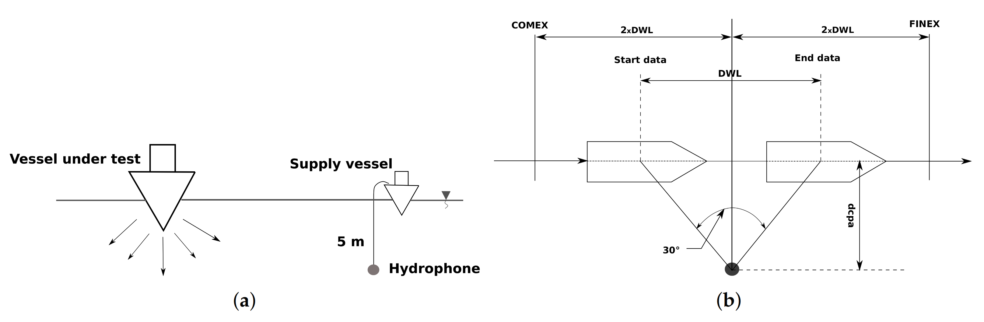
2. Data Collection

| Name | Type | Length | Breadth | Draught (fore) | Draught (aft) | Depth | Displacement |
|---|---|---|---|---|---|---|---|
| Nawigator XXI | Research vessel | 60.30 m | 10.50 m | 3.15 m | 3.20 m | 4.20 m | 1126 m3 |
| Propeller Type | Number | Pitch (%) | Blade Number | Model | Location from aft (Perpendicular) |
|---|---|---|---|---|---|
| CPP | 1 | 20–82% | 4 | abb zamech type p680/4-rps5000 | 3 m |
| conventional/clt/high skew |
| Engine Type | Number | Cylinder Number | Stroke Number | Reduction Gear Rate (RGR) | RPM |
|---|---|---|---|---|---|
| Diesel (Conventional) | 1 | 8 | 4 | 3.75 | 760 |
| Cylinder Firing Rate (CFR) | Engine Firing Rate (EFR) | Shaft Frequency (SF) | Blade Pass Frequency (BPF) |
|---|---|---|---|
| Hz | Hz | Hz | Hz |
| 6.3 | 50.7 | 3.37 | 13.51 |
3. Ship-Radiated Underwater Sound Analysis Methods
3.1. Power Spectral Density for Signal Energetics
3.2. Temporal Coherence Analysis for Tonal Signals
3.3. Frequency-Modulated Tonal Signal Analysis
3.4. Spectral Coherence Analysis for Cyclostationary Cavitation Noise
4. Results of the Ship Noise Analysis
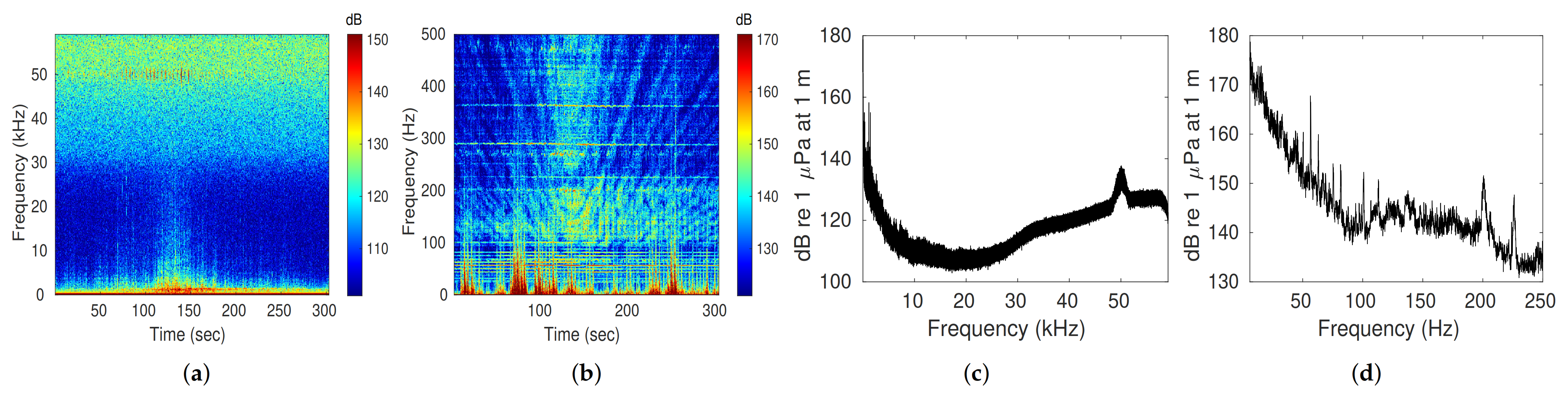
4.1. Ship Energetics via Power Spectral Density Analysis
4.2. Ship Tonal Signals via Temporal Coherence Analysis
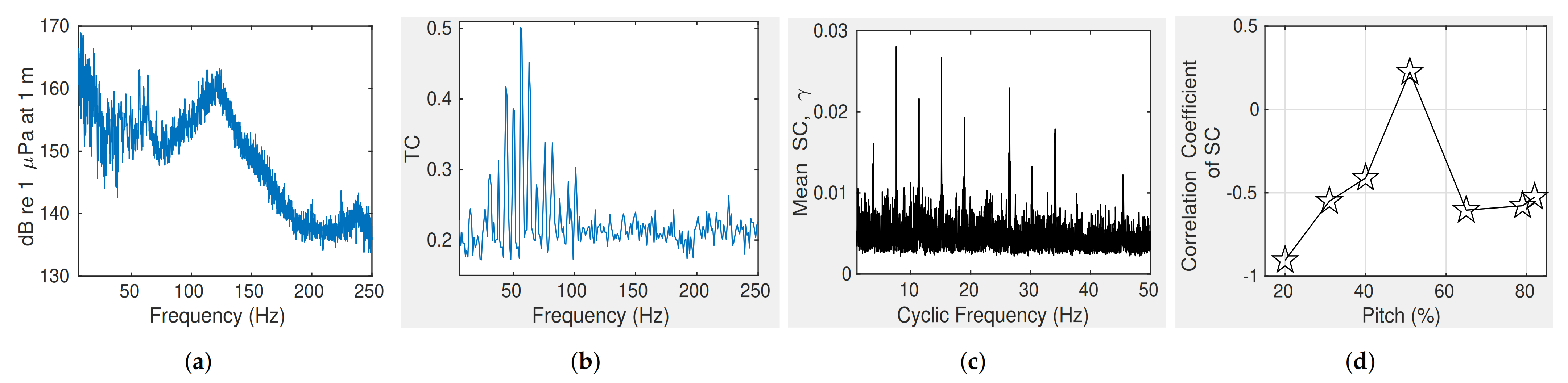
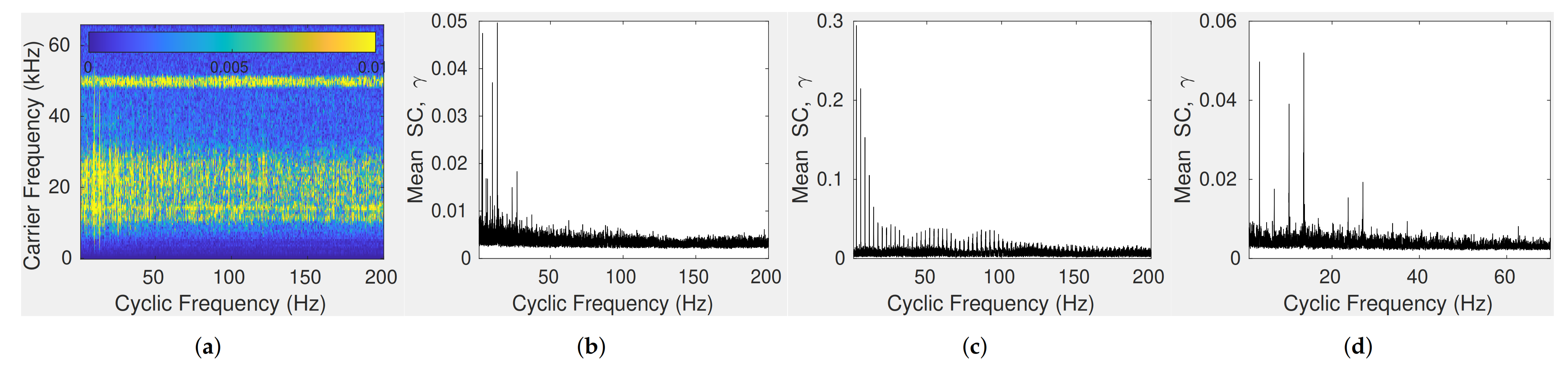
4.3. Cyclostationary Cavitation Noise via Spectral Coherence Analysis
5. A Comparison of the Ship’s Sound Characteristics at Different Propeller Pitches
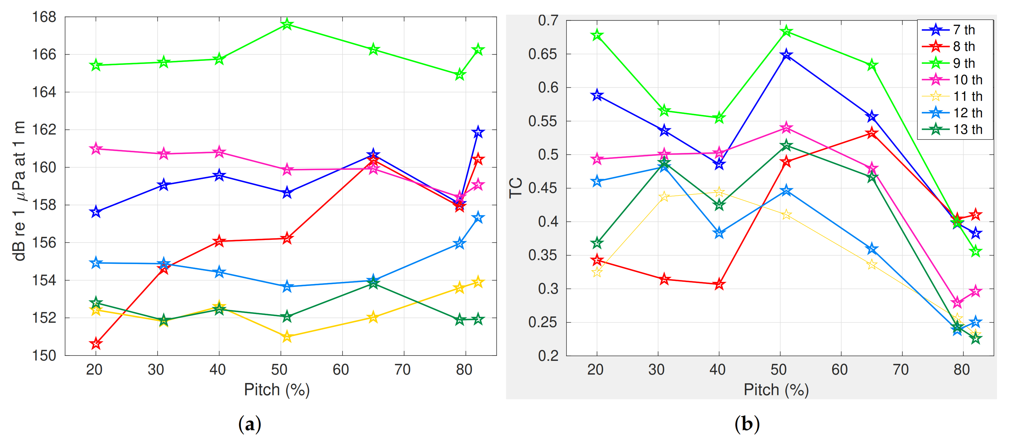
5.1. Power at Different Propeller Pitches
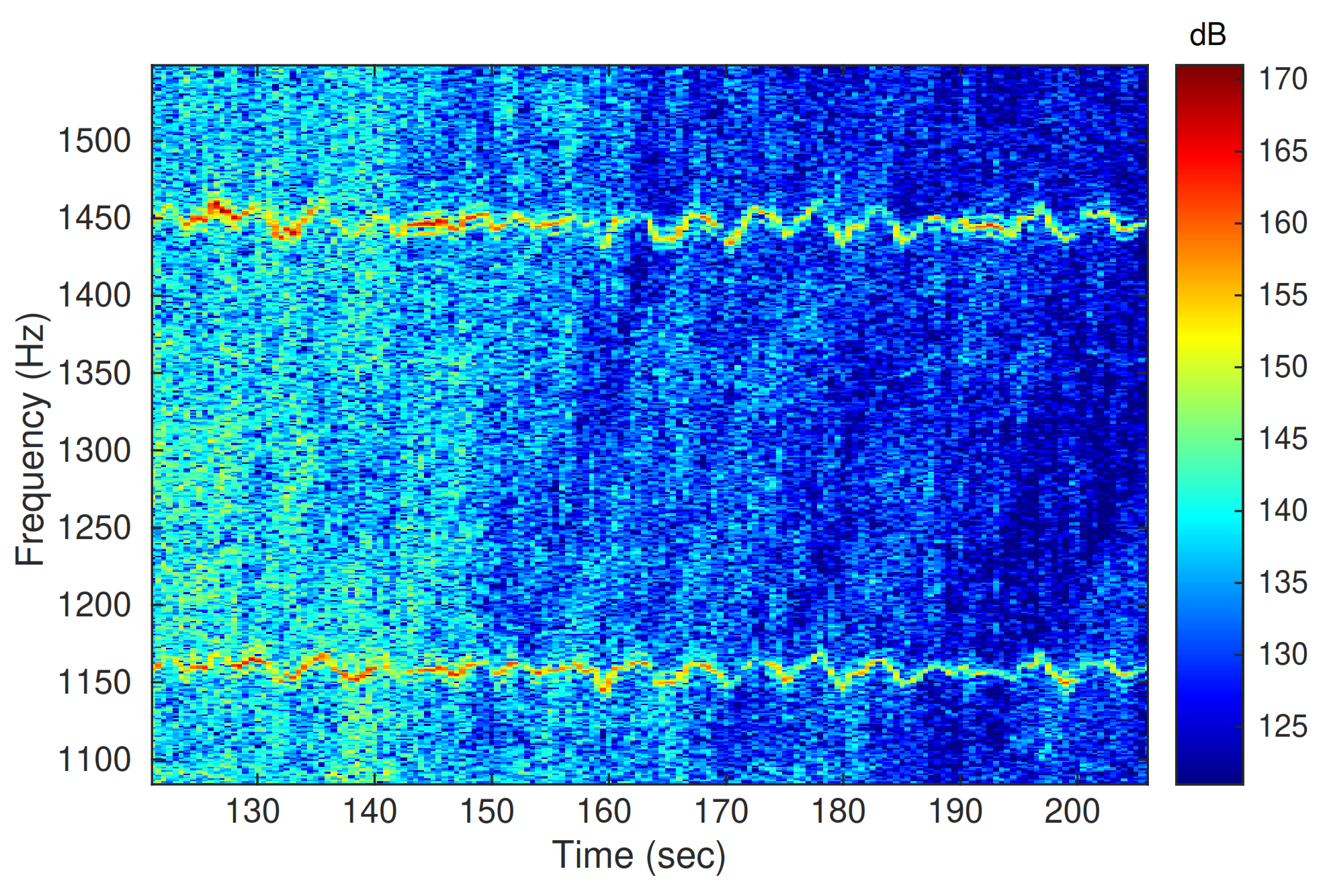
5.2. Tonal Signal Variations at Different Propeller Pitches
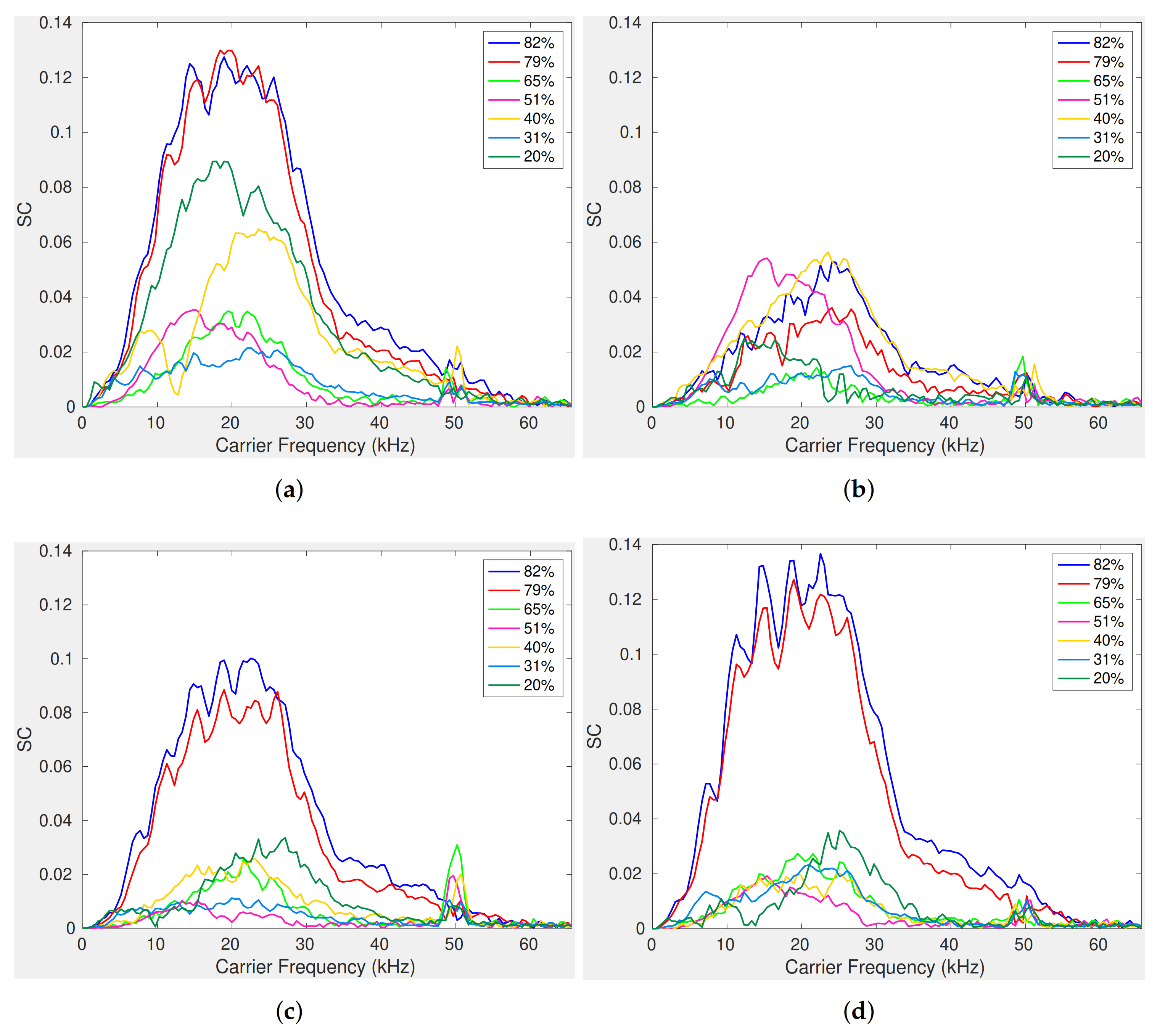
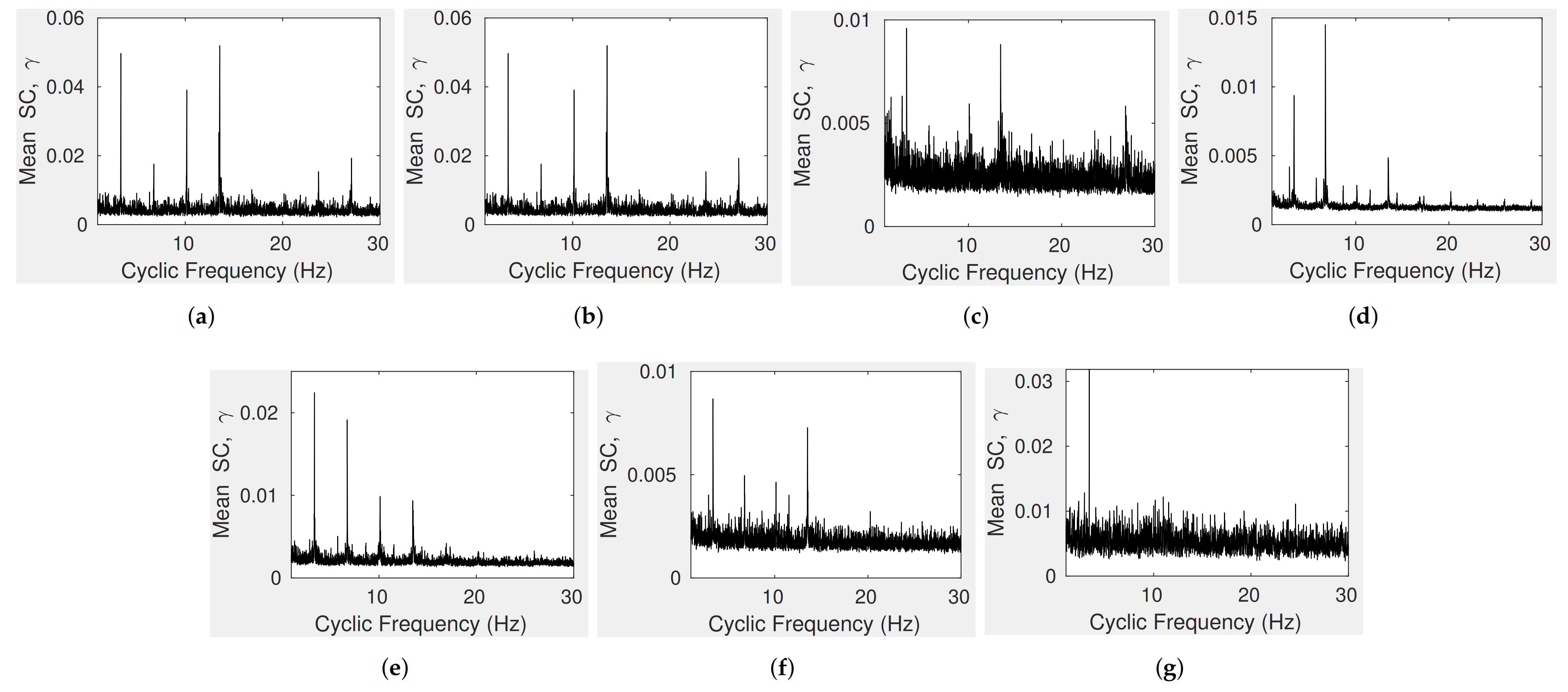
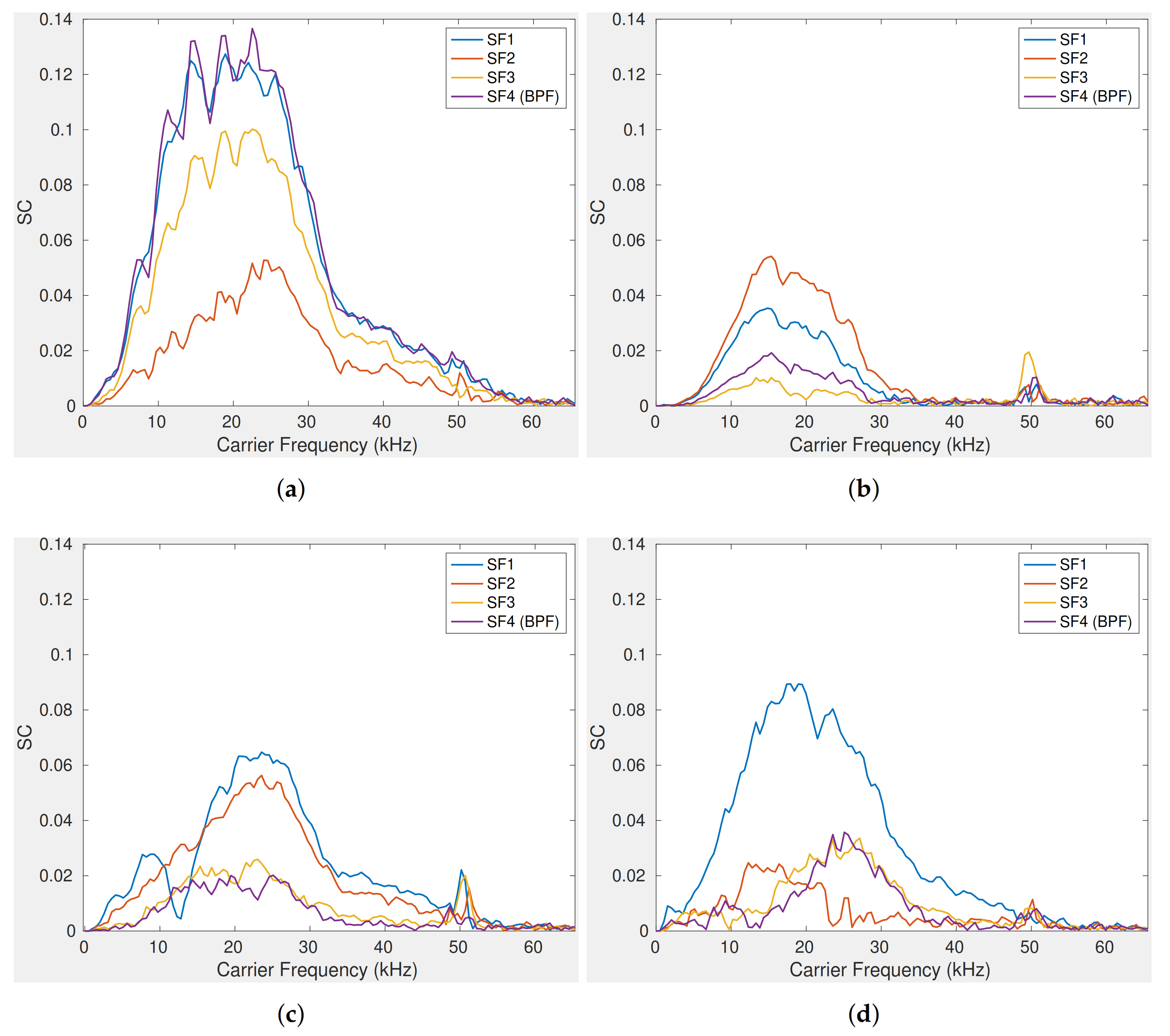
5.3. Propeller Cavitation Noise at Different Pitches
5.4. Robustness of the Estimation of Ship Parameters
5.4.1. Engine-Related Parameters
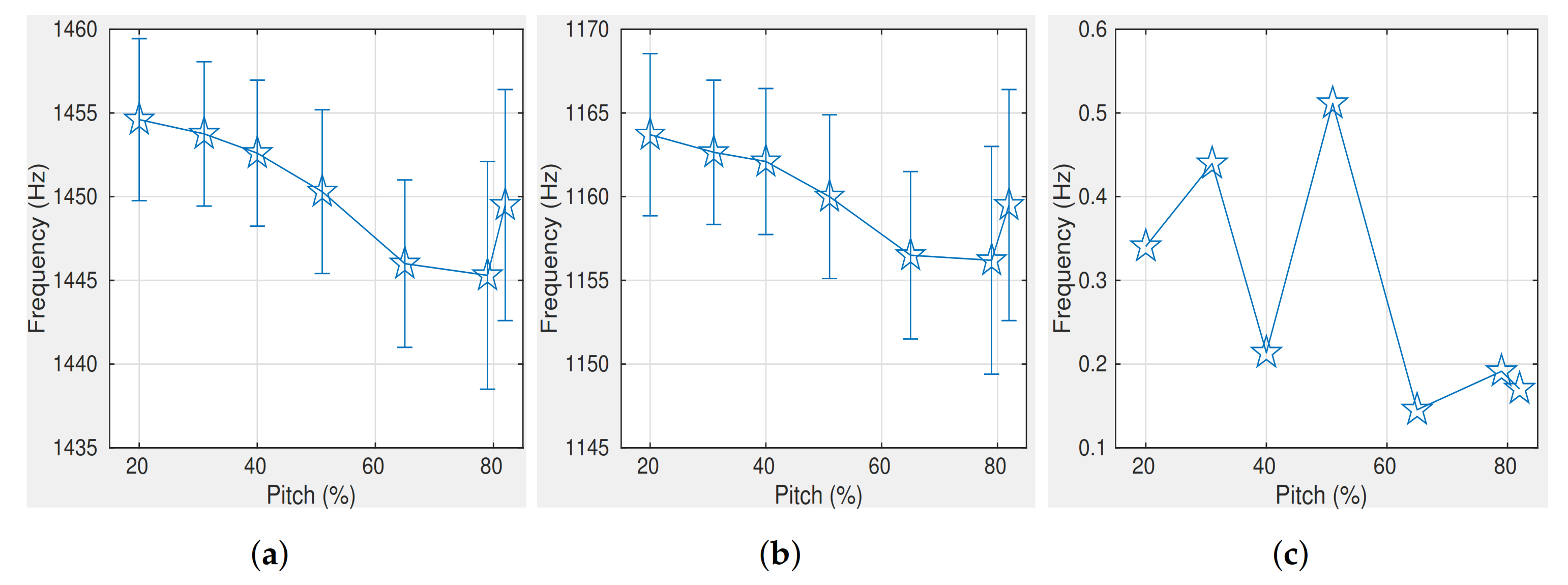
5.4.2. Propeller-Related Parameters
5.4.3. Gear-Related Parameters
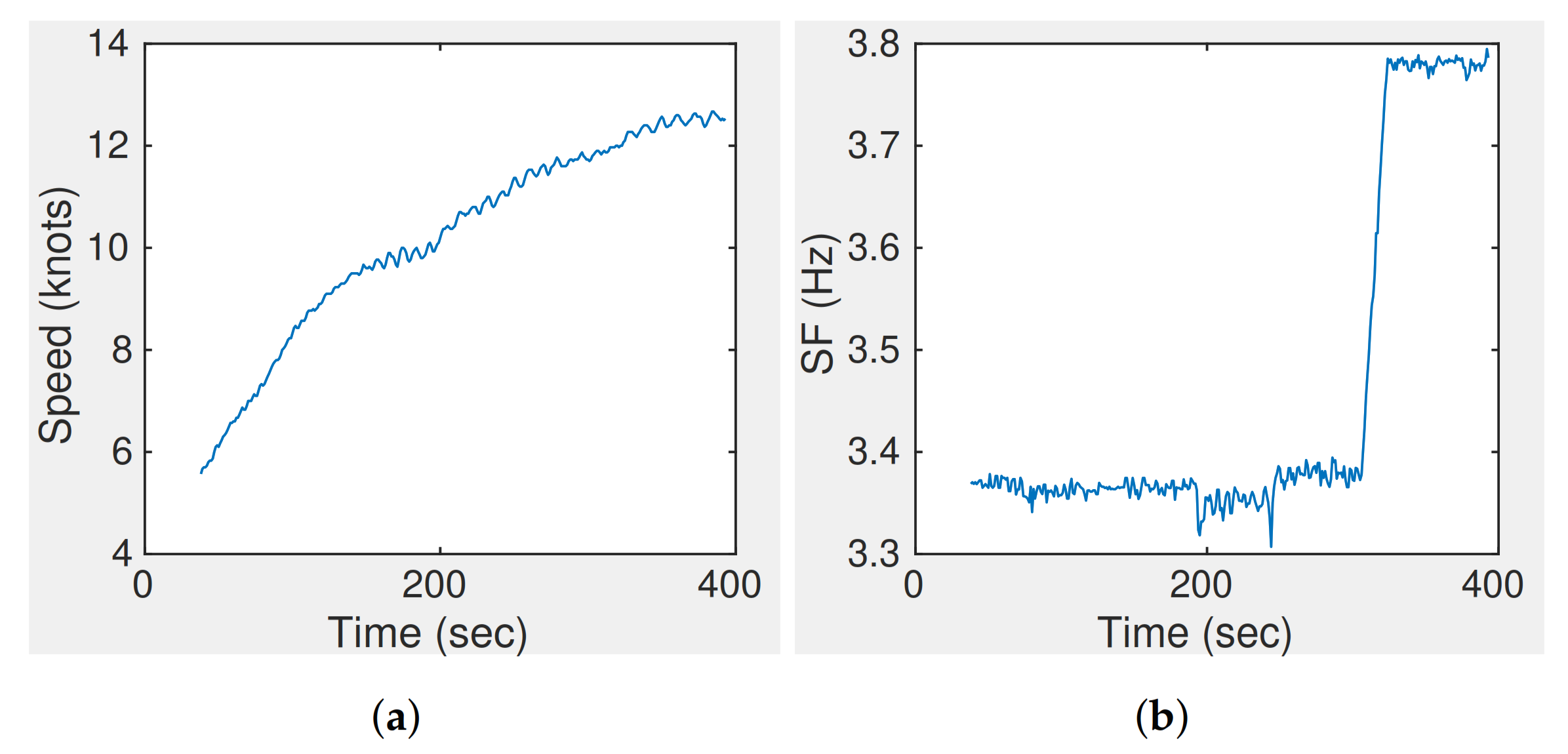
5.5. Changes in Both Propeller Pitch and RPM
6. Discussion
Author Contributions
Funding
Institutional Review Board Statement
Informed Consent Statement
Data Availability Statement
Conflicts of Interest
References
- Bergmann, P.G.; Major, J.; Wildt, R. Physics of Sound in the Sea; Gordon and Breach: London, UK, 1968. [Google Scholar]
- Arveson, P.T.; Vendittis, D.J. Radiated noise characteristics of a modern cargo ship. J. Acoust. Soc. Am. 2000, 107, 118–129. [Google Scholar] [CrossRef] [PubMed]
- Bruno, M.; Chung, K.; Salloum, H.; Sedunov, A.; Sedunov, N.; Sutin, A.; Graber, H.; Mallas, P. Concurrent use of satellite imaging and passive acoustics for maritime domain awareness. In Proceedings of the Waterside Security Conference (WSS), 2010 International, Carrara, Italy, 3–5 November 2010. [Google Scholar]
- Chung, K.W.; Sutin, A.; Sedunov, A.; Bruno, M. DEMON acoustic ship signature measurements in an urban harbor. Adv. Acoust. Vib. 2011, 2011. [Google Scholar] [CrossRef] [Green Version]
- Fillinger, L.; Sutin, A.; Sedunov, A. Acoustic ship signature measurements by cross-correlation method. J. Acoust. Soc. Am. 2010, 129, 774–778. [Google Scholar] [CrossRef] [PubMed]
- Leal, N.; Leal, E.; Sanchez, G. Marine vessel recognition by acoustic signature. ARPN J. Eng. Appl. Sci. 2015, 10, 9633–9639. [Google Scholar]
- Ogden, G.L.; Zurk, L.M.; Jones, M.E.; Peterson, M.E. Extraction of small boat harmonic signatures from passive sonar. J. Acoust. Soc. Am. 2011, 129, 3768–3776. [Google Scholar] [CrossRef] [Green Version]
- Wales, S.C.; Heitmeyer, R.M. An ensemble source spectra model for merchant ship-radiated noise. J. Acoust. Soc. Am. 2002, 111, 1211–1231. [Google Scholar] [CrossRef]
- Urick, R.J. Principles of Underwater Sound, 3rd ed.; Peninsula Publising: Los Atlos, CA, USA, 1983. [Google Scholar]
- Makris, N.C.; Ratilal, P.; Symonds, D.T.; Jagannathan, S.; Lee, S.; Nero, R.W. Fish population and behavior revealed by instantaneous continental shelf-scale imaging. Science 2006, 311, 660–663. [Google Scholar] [CrossRef]
- Makris, N.C.; Ratilal, P.; Jagannathan, S.; Gong, Z.; Andrews, M.; Bertsatos, I.; Godø, O.R.; Nero, R.W.; Jech, J.M. Critical population density triggers rapid formation of vast oceanic fish shoals. Science 2009, 323, 1734–1737. [Google Scholar] [CrossRef] [Green Version]
- Wang, D.; Garcia, H.; Huang, W.; Tran, D.D.; Jain, A.D.; Yi, D.H.; Gong, Z.; Jech, J.M.; Godø, O.R.; Makris, N.C.; et al. Vast assembly of vocal marine mammals from diverse species on fish spawning ground. Nature 2016, 531, 366–370. [Google Scholar] [CrossRef]
- Duane, D.; Cho, B.; Jain, A.D.; Godø, O.R.; Makris, N.C. The Effect of Attenuation from Fish Shoals on Long-Range, Wide-Area Acoustic Sensing in the Ocean. Remote Sens. 2019, 11, 2464. [Google Scholar] [CrossRef] [Green Version]
- Garcia, H.A.; Zhu, C.; Schinault, M.E.; Kaplan, A.I.; Handegard, N.O.; Godø, O.R.; Ahonen, H.; Makris, N.C.; Wang, D.; Huang, W.; et al. Temporal–spatial, spectral, and source level distributions of fin whale vocalizations in the Norwegian Sea observed with a coherent hydrophone array. ICES J. Mar. Sci. 2019, 76, 268–283. [Google Scholar] [CrossRef]
- Mohebbi-Kalkhoran, H.; Zhu, C.; Schinault, M.; Ratilal, P. Classifying humpback whale calls to song and non-song vocalizations using bag of words descriptor on acoustic data. In Proceedings of the 2019 18th IEEE International Conference On Machine Learning And Applications (ICMLA), IEEE, Boca Raton, FL, USA, 16–19 December 2019; pp. 865–870. [Google Scholar]
- Seri, S.G.; Zhu, C.; Schinault, M.; Garcia, H.; Handegard, N.O.; Ratilal, P. Long Range Passive Ocean Acoustic Waveguide Remote Sensing (POAWRS) of Seismo-Acoustic Airgun Signals Received on a Coherent Hydrophone Array. In Proceedings of the OCEANS 2019 MTS/IEEE SEATTLE, Seattle, WA, USA, 27–31 October 2019; pp. 1–8. [Google Scholar]
- MacLennan, D.N.; Simmonds, E.J. Fisheries Acoustics; Springer Science & Business Media: Berlin/Heidelberg, Germany, 2013; Volume 5. [Google Scholar]
- Vieira, M.; Amorim, M.; Sundelöf, A.; Prista, N.; Fonseca, P.J. Underwater noise recognition of marine vessels passages: Two case studies using hidden Markov models. ICES J. Mar. Sci. 2019, 77, 2157–2170. [Google Scholar] [CrossRef]
- Duane, D.; Zhu, C.; Piavsky, F.; Godø, O.R.; Makris, N.C. The Effect of Attenuation from Fish on Passive Detection of Sound Sources in Ocean Waveguide Environments. Remote Sens. 2021, 13, 4369. [Google Scholar] [CrossRef]
- Stojanovic, M. Underwater acoustic communications. In Proceedings of the Electro/95 International, Professional Program Proceedings, Boston, MA, USA, 21–23 June 1995; pp. 435–440. [Google Scholar]
- Stojanovic, M.; Preisig, J. Underwater acoustic communication channels: Propagation models and statistical characterization. IEEE Commun. Mag. 2009, 47, 84–89. [Google Scholar] [CrossRef]
- Dambra, R.; Firenze, E. Underwater radiated noise of a small vessel. In Proceedings of the 22nd International Congress on Sound and Vibration, Florence, Italy, 12–16 July 2015; pp. 12–16. [Google Scholar]
- Hildebrand, J.A. Anthropogenic and natural sources of ambient noise in the ocean. Mar. Ecol. Prog. Ser. 2009, 395, 5–20. [Google Scholar] [CrossRef] [Green Version]
- Merchant, N.D.; Witt, M.J.; Blondel, P.; Godley, B.J.; Smith, G.H. Assessing sound exposure from shipping in coastal waters using a single hydrophone and Automatic Identification System (AIS) data. Mar. Pollut. Bull. 2012, 64, 1320–1329. [Google Scholar] [CrossRef]
- Vasconcelos, R.O.; Amorim, M.C.P.; Ladich, F. Effects of ship noise on the detectability of communication signals in the Lusitanian toadfish. J. Exp. Biol. 2007, 210, 2104–2112. [Google Scholar] [CrossRef] [Green Version]
- Slabbekoorn, H.; Dooling, R.J.; Popper, A.N.; Fay, R.R. Effects of Anthropogenic Noise on Animals; Springer: Berlin/Heidelberg, Germany, 2018. [Google Scholar]
- Codarin, A.; Wysocki, L.E.; Ladich, F.; Picciulin, M. Effects of ambient and boat noise on hearing and communication in three fish species living in a marine protected area (Miramare, Italy). Mar. Pollut. Bull. 2009, 58, 1880–1887. [Google Scholar] [CrossRef]
- Ona, E.; Godø, O.R.; Handegard, N.O.; Hjellvik, V.; Patel, R.; Pedersen, G. Silent research vessels are not quiet. J. Acoust. Soc. Am. 2007, 121, EL145–EL150. [Google Scholar] [CrossRef] [Green Version]
- Mitson, R. Underwater noise radiated by research vessels. ICES Mar. Sci. Symp. 1993, 196, 147–152. [Google Scholar]
- Mitson, R.B.; Knudsen, H.P. Causes and effects of underwater noise on fish abundance estimation. Aquat. Living Resour. 2003, 16, 255–263. [Google Scholar] [CrossRef]
- Hawkins, A.D.; Pembroke, A.E.; Popper, A.N. Information gaps in understanding the effects of noise on fishes and invertebrates. Rev. Fish Biol. Fish. 2015, 25, 39–64. [Google Scholar] [CrossRef]
- Veirs, S.; Veirs, V.; Wood, J.D. Ship noise extends to frequencies used for echolocation by endangered killer whales. PeerJ 2016, 4, e1657. [Google Scholar] [CrossRef] [Green Version]
- Erbe, C.; Dunlop, R.; Dolman, S. Effects of noise on marine mammals. In Effects of Anthropogenic Noise on Animals; Springer: Berlin/Heidelberg, Germany, 2018; pp. 277–309. [Google Scholar]
- Fréchou, D.; Dugué, C.; Briançon-Marjollet, L.; Fournier, P.; Darquier, M.; Descotte, L.; Merle, L. Marine Propulsor Noise Investigations in the Hydroacoustic Water Tunnel “GTH”. In Proceedings of the Twenty-Third Symposium on Naval Hydrodynamics, Val de Reuil, France, 17–22 September 2000; Office of Naval Research Bassin d’Essais des Carenes National Research Council: Washington, DC, USA, 2001. [Google Scholar]
- Bush, V.; Conant, J.B.; Tate, J.T. Principles and Applications of Underwater Sound; Technical Report; Office of Scientific Research and Development: Washington, DC, USA, 1946; Volume 7. [Google Scholar]
- Norwood, C. An introduction to ship radiated noise. Acoust. Aust. 2002, 30, 21–25. [Google Scholar]
- Ojak, W. Vibrations and waterborne noise on fishery vessels. J. Ship Res. 1988, 32, 112–133. [Google Scholar] [CrossRef]
- Gray, L.M.; Greeley, D.S. Source level model for propeller blade rate radiation for the world’s merchant fleet. J. Acoust. Soc. Am. 1980, 67, 516–522. [Google Scholar] [CrossRef]
- Grelowska, G.; Kozaczka, E.; Kozaczka, S.; Szymczak, W. Underwater noise generated by a small ship in the shallow sea. Arch. Acoust. 2013, 38, 351–356. [Google Scholar] [CrossRef]
- Zhu, C.; Seri, S.G.; Mohebbi-Kalkhoran, H.; Ratilal, P. Long-range automatic detection, acoustic signature characterization and bearing-time estimation of multiple ships with coherent hydrophone array. Remote Sens. 2020, 12, 3731. [Google Scholar] [CrossRef]
- Zhu, C. Remote Monitoring of Multiple Ships over Instantaneous Continental-Shelf Scale Region with Large-Aperture Coherent Hydrophone Array. Ph.D. Thesis, Northeastern University, Boston, MA, USA, 2020. [Google Scholar]
- Malinowski, S.J.; Gloza, I. Underwater noise characteristics of small ships. Acta Acust. United Acust. 2002, 88, 718–721. [Google Scholar]
- Gloza, I. Identification Methods of Underwater Noise Sources Generated by Small Ships. Acta Phys. Pol. A. 2011, 119. [Google Scholar] [CrossRef]
- McKenna, M.F.; Ross, D.; Wiggins, S.M.; Hildebrand, J.A. Underwater radiated noise from modern commercial ships. J. Acoust. Soc. Am. 2012, 131, 92–103. [Google Scholar] [CrossRef] [PubMed] [Green Version]
- Antoni, J.; Hanson, D. Detection of surface ships from interception of cyclostationary signature with the cyclic modulation coherence. IEEE J. Ocean. Eng. 2012, 37, 478–493. [Google Scholar] [CrossRef]
- Hanson, D.; Antoni, J.; Brown, G.; Emslie, R. Cyclostationarity for ship detection using passive sonar: Progress towards a detection and identification framework. In Proceedings of the ACOUSTICS 2009, Adelaide, SA, Australia, 23–25 November 2009; pp. 1–8. [Google Scholar]
- Zhu, C.; Garcia, H.; Kaplan, A.; Schinault, M.; Handegard, N.O.; Godø, O.R.; Huang, W.; Ratilal, P. Detection, localization and classification of multiple mechanized ocean vessels over continental-shelf scale regions with passive ocean acoustic waveguide remote sensing. Remote Sens. 2018, 10, 1699. [Google Scholar] [CrossRef] [Green Version]
- Huang, W.; Wang, D.; Garcia, H.; Godø, O.R.; Ratilal, P. Continental shelf-scale passive acoustic detection and characterization of diesel-electric ships using a coherent hydrophone array. Remote Sens. 2017, 9, 772. [Google Scholar] [CrossRef] [Green Version]
- Gaggero, T.; Rizzuto, E.; Traverso, F.; Trucco, A. Comparing ship underwater noise measured at sea with predictions by empirical models. In Proceedings of the 21st International Congress on Sound and Vibration, Beijing, China, 13–17 July 2014; pp. 1510–1516. [Google Scholar]
- Traverso, F.; Gaggero, T.; Tani, G.; Rizzuto, E.; Trucco, A.; Viviani, M. Parametric analysis of ship noise spectra. IEEE J. Ocean. Eng. 2016, 42, 424–438. [Google Scholar] [CrossRef]
- Traverso, F.; Gaggero, T.; Rizzuto, E.; Trucco, A. Spectral analysis of the underwater acoustic noise radiated by ships with controllable pitch propellers. In Proceedings of the OCEANS 2015-Genova, Genova, Italy, 18–21 May 2015; pp. 1–6. [Google Scholar]
- AQUO. Achieve QUieter Oceans by Shipping Noise Footprint Reduction. Available online: www.aquo.eu (accessed on 8 January 2022).
- ANSI/ASA. S12.64-2009/Part 1, Quantities and Procedures for Description and Measurement of Underwater Sound from Ship—Part 1: General Requirements. 2009. Available online: https://webstore.ansi.org/standards/asa/ansiasas12642009partr2014 (accessed on 8 January 2022).
- Welch, P. The use of fast Fourier transform for the estimation of power spectra: A method based on time averaging over short, modified periodograms. IEEE Trans. Audio Electroacoust. 1967, 15, 70–73. [Google Scholar] [CrossRef] [Green Version]
- Goodman, J. Statistical Optics; Willey: New York, NY, USA, 1988. [Google Scholar]
- Kay, S.M. Modern Spectral Estimation; Prentice Hall: Hoboken, NJ, USA, 1988. [Google Scholar]
- Shapiro, A.D.; Wang, C. A versatile pitch tracking algorithm: From human speech to killer whale vocalizations. J. Acoust. Soc. Am. 2009, 126, 451–459. [Google Scholar] [CrossRef] [Green Version]
- Baumgartner, M.F.; Mussoline, S.E. A generalized baleen whale call detection and classification system. J. Acoust. Soc. Am. 2011, 129, 2889–2902. [Google Scholar] [CrossRef] [Green Version]
- Antoni, J. Cyclostationarity by examples. Mech. Syst. Signal Process. 2009, 23, 987–1036. [Google Scholar] [CrossRef]
- Antoni, J.; Xin, G.; Hamzaoui, N. Fast computation of the spectral correlation. Mech. Syst. Signal Process. 2017, 92, 248–277. [Google Scholar] [CrossRef]
- Gardner, W. Measurement of spectral correlation. IEEE Trans. Acoust. Speech Signal Process. 1986, 34, 1111–1123. [Google Scholar] [CrossRef]
- Pollara, A.; Sutin, A.; Salloum, H. Improvement of the Detection of Envelope Modulation on Noise (DEMON) and its application to small boats. In Proceedings of the OCEANS 2016 MTS/IEEE Monterey, Monterey, CA, USA, 19–23 September 2016; pp. 1–10. [Google Scholar]
- Boashash, B.; O’shea, P. A methodology for detection and classification of some underwater acoustic signals using time-frequency analysis techniques. IEEE Trans. Acoust. Speech Signal Process. 1990, 38, 1829–1841. [Google Scholar] [CrossRef] [Green Version]
- Pollara, A.; Sutin, A.; Salloum, H. Modulation of high frequency noise by engine tones of small boats. J. Acoust. Soc. Am. 2017, 142, EL30–EL34. [Google Scholar] [CrossRef] [Green Version]
- Hanson, D.; Antoni, J.; Brown, G.; Emslie, R. Cyclostationarity for passive underwater detection of propeller craft: A development of DEMON processing. In Proceedings of the Acoustics 2008, Geelong, VIC, Australia, 24–26 November 2008; pp. 24–26. [Google Scholar]


| Pitch (%) | 82 | 79 | 65 | 51 | 40 | 31 | 20 |
|---|---|---|---|---|---|---|---|
| SF1 (SF) | ✓ | ✓ | ✓ | ✓ | ✓ | ✓ | ✓ |
| SF2 | ✓ | ✓ | × | ✓ | ✓ | ✓ | × |
| SF3 | ✓ | ✓ | ✓ | ✓ | ✓ | ✓ | × |
| SF4 (BPF) | ✓ | ✓ | ✓ | ✓ | ✓ | ✓ | × |
| Blade Number | ✓ | ✓ | ✓ | × | × | ✓ | × |
Publisher’s Note: MDPI stays neutral with regard to jurisdictional claims in published maps and institutional affiliations. |
© 2022 by the authors. Licensee MDPI, Basel, Switzerland. This article is an open access article distributed under the terms and conditions of the Creative Commons Attribution (CC BY) license (https://creativecommons.org/licenses/by/4.0/).
Share and Cite
Zhu, C.; Gaggero, T.; Makris, N.C.; Ratilal, P. Underwater Sound Characteristics of a Ship with Controllable Pitch Propeller. J. Mar. Sci. Eng. 2022, 10, 328. https://doi.org/10.3390/jmse10030328
Zhu C, Gaggero T, Makris NC, Ratilal P. Underwater Sound Characteristics of a Ship with Controllable Pitch Propeller. Journal of Marine Science and Engineering. 2022; 10(3):328. https://doi.org/10.3390/jmse10030328
Chicago/Turabian StyleZhu, Chenyang, Tomaso Gaggero, Nicholas C. Makris, and Purnima Ratilal. 2022. "Underwater Sound Characteristics of a Ship with Controllable Pitch Propeller" Journal of Marine Science and Engineering 10, no. 3: 328. https://doi.org/10.3390/jmse10030328
APA StyleZhu, C., Gaggero, T., Makris, N. C., & Ratilal, P. (2022). Underwater Sound Characteristics of a Ship with Controllable Pitch Propeller. Journal of Marine Science and Engineering, 10(3), 328. https://doi.org/10.3390/jmse10030328