Abstract
Offshore wind farms have developed rapidly in Jiangsu Province, China, over the last decade. The existence of offshore wind turbines will inevitably impact hydrological and sedimentary environments. In this paper, a digital elevation model (DEM) of the intertidal sandbank in southern Jiangsu Province from 2018 to 2020 was constructed based on the improved remote sensing waterline method. On this basis, the stability of the sandbank was analysed, and combined with the hypothetical sandbank surface discrimination method (HSSDM), the erosional/depositional influences of wind turbine construction on topography were quantitatively analysed. The results show that due to the frequent oscillations of the tidal channels, only 35.03% of the study area has a stable topography, and more than 90% of the wind turbines in all years have a balanced impact on the intensity of topographic change, and all see a small reduction in their impact in the following year. The remaining wind turbines with erosional/depositional impacts are mainly located in areas with unstable topography, but the overall impact of all wind turbines is balanced in 2018–2020. The impact of wind turbines on topography is both erosional and depositional, but the overall intensity of the impact is not significant. This study demonstrates the quantitative effects of wind turbine construction on topography and provides some help for wind turbine construction site selection and monitoring after turbine completion.
1. Introduction
Wind energy is conducive to the development of green and clean energy and is one of the most important energy transitions for achieving carbon neutrality [1,2]. Offshore wind power construction not only makes full use of offshore wind energy but also saves land resources and is a key focus of new energy development [3]. At present, technology for Chinese offshore wind power is mainly built in offshore waters [4]. China is leading the world in terms of annual installed offshore wind capacity, and in 2021, overtook the UK as the world’s top offshore wind market, thereby entering a new phase of offshore wind development.
Tidal flats are the most active areas of the land–sea interface and play an important role in the ecological and economic development of the region [5]. Jiangsu has abundant tidal flat resources [6], and the offshore radial sandy ridge and its onshore tidal flats have great development and utilization value as important reserve land resources in the intertidal zone of Jiangsu [7,8]. At the same time, the shallow waters and low slope of the ocean bottom in Jiangsu offer topographical advantages in offshore wind power construction [9]. By the end of September 2021, the cumulative grid-connected capacity of offshore wind power in Jiangsu was 7.25 million kilowatts, accounting for more than 70% of the national total, making it the number one province in the country in terms of cumulative grid-connected capacity. However, offshore wind farms are usually large in scale, and their construction and operation will inevitably have some impact on local hydrology [10] and habitats [11,12,13]. The identification of the remote sensing images revealed that some of the wind turbines were connected to tidal channels which were previously undeveloped and formed. The installation of wind turbines will expose the topography to anthropogenic influences in addition to natural ones such as waves and currents. It is therefore necessary to monitor changes in tidal flats and to analyse the impacts of wind turbine construction in a timely manner.
Current research on wind power construction focuses on the infrastructure [14,15] and construction conditions [16] of offshore wind farms. The offshore wind environment is unique, and people mainly obtain research data on it through offshore field investigations [16] or laboratory modelling [13,14,15,16,17]. In addition, professional software is used for numerical simulations [18,19] or remote sensing data [4] to analyse the wind field or hydrodynamic characteristics of offshore turbines, and the main research method is numerical simulation [20]. However, studies on the impact of offshore wind power in tidal areas on the topographic environment and other effects are still relatively scarce.
Tidal flats are influenced by environmental factors and have complex topographic conditions [21]. There are already a few studies focused on monitoring changes oriented towards tidal flat areas [22,23,24]. In contrast, tidal flat areas make it difficult to carry out large-scale in situ real-time observations due to periodic inundation [25]. Thus, optical remote sensing images are increasingly becoming an important resource for monitoring historical changes in tidal flat morphology and the impact of wind turbines on topography [26,27]. Mason et al. (1998) [28] proposed constructing a digital elevation model of tidal flats by considering the waterlines in remote sensing images as contour lines. Subsequently, several scholars used remote sensing images for tidal flat DEM (digital elevation model) construction by combining water edge line extraction with other methods, such as the irregular triangular network method [29], time series method [30] and BP neural network model [31].
The proper construction and use of DEMs is key to analysing the interactions between wind turbines and topography. The tidal flat DEM constructed by the current method can present the overall features of the topography, but it is difficult to show the micro-geomorphic features of the tidal channels effectively. In intertidal regions, tidal channels are important topographic elements and have an important impact on the construction and operation of offshore wind turbines. There is also a need to explore how to fully utilize the DEM to study the association of topographic features with the effects generated by wind turbines.
Therefore, the main objectives of this paper are: (1) to use an improved DEM construction method to obtain a DEM capable of featuring the micro-geomorphology of intertidal wind farms, (2) to analyse the topographic stability characteristics of the study area using the DEM, and (3) to quantitatively assess the impact of wind turbine construction and operation on intertidal topography in terms of erosion and deposition using the DEM. It is hoped that this will provide some assistance in the construction and monitoring of wind turbines.
The remainder of the paper is structured as follows: In Section 2, we introduce the natural conditions and hydrodynamic characteristics of the study area and datasets used in the paper, including the satellite image data, hydrographic data, and wind turbine data. Our research technique is shown in Section 3. In Section 4, Section 5 and Section 6, the DEM construction method, the sandbank stability discriminant method, and the topographic change intensity (TCI) assessment method are briefly described, as well as their corresponding results. In Section 7, we analyse the effects of the wind turbine on topography and compared them with the results obtained by the semitheoretical formula. Our conclusions are drawn in Section 8.
2. Study Area and Datasets
2.1. Study Area
In this paper, the wind farm of the southern radial sandy ridge (RSR) is used as the DEM construction study area (Figure 1). The RSR is located on the outer edge of the northern Jiangsu coast. Over the last 40 years, the large tidal flats in the RSR have been subjected mainly to erosion. Smaller tidal flats are shifting under the influence of tidal channels [27]. The tide levels in the study area are mainly monitored by the tidal stations at Dafenggang, Jianggang and Yangkougang. Within the area, the tides are mainly semidiurnal with a tide range varying from 2.5 to 4.0 m and a water depth range varying from 0 to 30 m [26]. The tide currents in the study area are important. They are the main driver of water flow and have a large influence on the suspended sediment concentration [32]. Controlled by tidal currents, a series of radial submerged sand ridges are developed in the offshore area of the southern Yellow Sea [33]. The RSR of the Jiangsu coast provides a rich source of erosional material for coastal tidal development, and the cover created by the large body of sand provides protection for nearshore mudflat development [7]. The RSR has a large number of tidal channels and is an important site for fisheries production activities. It is also a key area for the construction of the offshore wind power industry, with several offshore wind farms. The radiating topography and the special tidal field also make the wave characteristics of the sea variable.
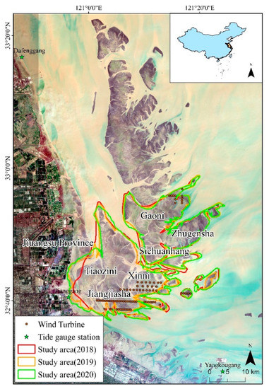
Figure 1.
Location map of the study area showing the distribution of tidal gauge stations and wind turbines. (Differently coloured boxes indicate the extent of the constructed DEM for the corresponding year; asterisks indicate the locations of tidal gauge stations; dots indicate wind turbine locations).
2.2. Datasets
2.2.1. Satellite Image Data
Image data from three main sensors were used in this study: Sentinel-2 MSI, Landsat-7 Enhanced Thematic Mapper Plus (ETM+), and Landsat 8 OLI. The spatial resolutions were 10 m, 30 m and 30 m, respectively. The requirements for this remote sensing imagery include clear images, low cloud content and tide levels that vary by image. A total of 54 scenes from 2018 to 2020 were finally used as remote sensing data sources. All images were preprocessed with atmospheric and geometric corrections and projected using UTM WGS84 (51° N).
2.2.2. Hydrographic Data
In this study, tide level data (http://global-tide.nmdis.org.cn/, accessed on 7 February 2022) were collected from Dafenggang, Jianggang and Yangkougang from June 2018 to January 2019. The tidal reconciliation constants were calculated based on the principle of tidal harmonic analysis [34] to calculate the tide level at the moment of remote sensing image collection. The tide level calculation results had good accuracy. In addition, hydrological data, such as sand concentration, sedimentation rate and flow velocity, were obtained from the hydrological test reports of the study area so that the thickness of erosion or deposition was calculated using semitheoretical formulas.
2.2.3. Wind Turbine Data
There are several existing offshore wind farm projects in the study area, such as the Longyuan Jiangsu Jiangjiasha 300 MW offshore wind farm project and Guohua Zhugensha (H1#) offshore wind farm project. The majority of these turbines were installed in 2017–2018 and grid connected operation started in 2018. The availability of offshore wind turbines is currently over 90% [35]. This means that wind turbines are running almost all the time, which will put the environment at constant risk.
Using the 2018 ESA Sentinel satellite remote sensing Sentinel-2 image for discrimination, 82 offshore wind turbine locations, which are mainly distributed in the eastern and southern parts of the study area, were extracted, and the specific distribution locations are shown in Figure 1. The average intervals between wind turbines are mainly 500 or 1000 m.
3. Research Technique
The DEM of the wind farm is the basis for the hypothetical sandbank surface discrimination method (HSSDM) in the absence of wind turbines. We improved the remote sensing waterline method to obtain a more refined tidal topography (Section 4), making full use of the DEM for topography stability analysis (Section 5) and using the HSSDM (Section 6) to analyse and assess the intertidal zone erosion, deposition status and intensity caused by the construction of wind turbines for long-term sustainable assessment; the technical flow chart is shown in Figure 2.
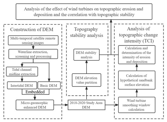
Figure 2.
Flow chart of the research technology.
4. DEM Construction of Intertidal Wind Farms
The current waterline method is the main method of building a tidal flat DEM. Using the waterline method, a DEM can be constructed by establishing the relationship between the waterline and the tide level. However, two issues affect the construction and use of the DEM: one is the misplaced waterlines, and the other is the presentation of the tidal channel micro-geomorphology. Therefore, this study improves DEM accuracy through waterline sequencing and tidal channel embedding.
4.1. DEM Construction Method
4.1.1. Waterline Sequencing and Initial DEM Construction
The waterline is the water–land boundary extracted from the remote sensing image. The area surrounded by the waterline can indicate the tidal flat area, while the elevation of the waterline can be indicated by the tide level. Therefore, the higher the tide level is, the smaller the area of exposed tidal flats that can be exploited, but this is often ignored in conventional terrain construction. In this paper, the tide ranking is added, and the waterlines with correct spatial and tide level relationships are screened for subsequent DEM interpolation construction by combining the waterline variation pattern. The specific steps are as follows:
a. Waterline edges in images were extracted using the modified normalized difference water index (MNDWI) combined with visual interpretation; b. using the tidal ranking of Yangkougang as a benchmark, the images of the study area taken in each year were ranked and combined with the pattern of waterline changes to filter out the waterlines with the correct spatial and tidal relationship; c. discrete points were taken at 30 m intervals along the waterline by ArcGIS software; d. tidal simulation was completed using the T_TIDE tool to obtain the tidal level at each image moment at each station and the discrete point elevation at each waterline by the inverse distance weighting (IDW) method; e. the initial intertidal DEM of the study area was constructed using the kriging difference method.
4.1.2. DEM Micro-Geomorphic Feature Enhancement
The regional distribution of the wind turbines in the study area and the extent of the siltation influence are relatively small. The initial DEM can show the overall topographic trend of the study area, but tidal channels with micro-geomorphic features are smoothed out during the interpolation process, and micro-geomorphic features can be enhanced using tidal channel embedding. The specific steps are as follows:
a. Images with the lowest tide levels and clear tidal channels in each year were selected, and tidal channel boundaries and their middle lines were extracted and discretized by 30 m; b. the same method as above was used to assign values to the discreted points of the tidal channel boundaries; c. the values of discrete points from middle lines were assigned by the IDW method using the lowest tide level at Yangkougang for each year; d. discrete points were interpolated using the kriging method, a tidal channel DEM was obtained by extraction via a mask, and the initial intertidal DEM was embedded to complete the topography of the study area.
The method was obtained by a validation profile comparison for better topographic accuracy by Zhou (2021) [36] (RMSE = 0.54 m). It also has good consistency in the varying profile undulation patterns.
4.2. DEM Results
Through the method described in Section 4.1, the waterlines extracted from the images taken each year were interpolated. The final DEM of the study area for 2018–2020 at a 30 m spatial resolution was constructed and improved, as shown in Figure 3a–c. The spatial distribution of the DEM indicates each sandbank, which shows the topographic characteristics of an island-type sandbar with a high centre and low surroundings, and the beach surface is mostly distributed with small tidal channels. The central part of Tiaozini and the western part of Gaoni are both areas with higher DEMs in all years. Zhugensha is divided into strips of sand by tidal channels. Sichuanhang is affected by the development of its central tidal channel, and the north–south division is gradually obvious. The western side of Xinni is also an area with a higher elevation, while the eastern side is relatively flat and open.
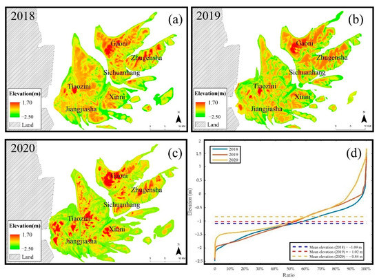
Figure 3.
DEMs of the study area for 2018–2020 using the methods described above. ((a–c) DEM construction results for each year; (d) DEM elevation frequency histogram results for each year.)
The statistical areas in each year are 750.75 km2, 754.98 km2, and 814.75 km2. The lowest DEM elevations are similar in each year; the elevations are −2.48 m, −2.42 m and −2.35 m. The highest DEM elevations are similar in 2018 and 2020, with values of 1.67 and 1.68 m, respectively, while there is a significant decrease in 2019, with a value of 1.37 m. Although the maximum DEM elevation fluctuates, the average elevation increases from −1.09 m to −1.02 m to −0.84 m, showing an increasing annual trend. The percentages of elevation values in each year, as shown in Figure 3d, are basically the same, showing a “Z” shape. The elevation values change almost vertically at both ends, while the middle elevation values change more moderately, indicating that there are fewer topographic extreme areas and that the rest of the elevations are more evenly distributed. The 2020 elevation values are higher in almost all percentages than in the previous two years. The 2019 elevation values are significantly higher than the 2018 elevation values by approximately 45%.
5. Stability Analysis of the Sandbank
We explored the topographic stability of the study area before investigating the effect of wind turbines on topographic siltation. The construction of external turbines is an important factor that influences flushing and siltation, but the stability characteristics of the sand body itself are also worth studying. Therefore, topographic elevation zoning and stability analysis were carried out by accounting for the changes in elevation values over three years.
5.1. Sandbank Stability Discriminant Method
The elevations of the DEM results in Section 4.2 were divided into different elevation zones based on the 0.5 m, −0.5 m and −1.5 m contours of each DEM. The stability of the sandbank was then determined by the number of elevation zones to which the elevation of the same raster belongs in each year and whether the elevation zones are continuous, as follows:
- (a)
- The sandbank is classified as stable if the elevations are in the same elevation zone for three years.
- (b)
- The sandbank is classified as unstable if the elevations are in two elevation zones and the two elevation zones are continuous for three years (e.g., “elevation < −1.5 m” and “−1.5 < elevation < −0.5”).
- (c)
- The sandbank is classified as very unstable if the elevations are in two elevation zones and the two elevation zones are discontinuous for three years (e.g., “elevation value < −1.5” and “−0.5 < elevation value < 0.5”), or if the elevations are in three elevation zones for three years.
Sandbank stability was assessed on the basis of the DEM delineation results for each year. The stable and unstable results were ranked according to their elevation relationships. A total of eight results were obtained and classified by assigning values from 1 to 8. Areas with values of 1, 3, 5 and 7 are stable; areas with values of 2, 4 and 6 are unstable; areas with a value of 8 are very unstable; and all areas are ordered from the lowest to highest elevations.
5.2. Sandbank Stability Status
The results of the 2018–2020 DEM elevation zones are shown in Figure 4a–c. By using statistical calculations, from −1.5~−0.5 m, the area is the largest in all years, and more than 50% of the terrain is smaller than the −0.5 m contour in all years. The smallest terrain area is greater than the 0.5 m contour in 2018 and 2019, accounting for less than 1% of both. The smallest terrain area in 2020 is the area with a contour less than −1.5 m, accounting for 4.32%.
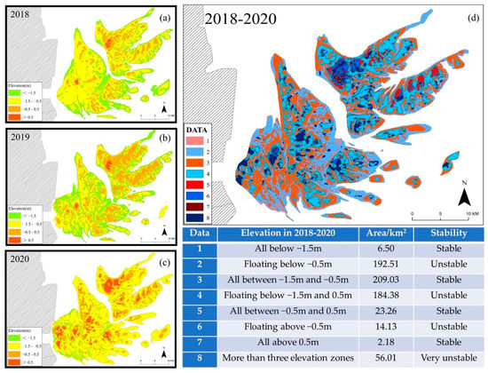
Figure 4.
Elevation zone results and stability determination results for the 2018–2020 study area. ((a–c) Zone results for DEM elevation values for each year; (d) sandbank stability determination results for the study area; the table in the lower right corner shows the meaning and area of the values in (d)).
As shown in Figure 4d, the regions with values of 1, 3, 5 and 7 in the figure, where the topographic zoning remains unchanged over a three-year period, can be considered as the more stable regions. Other values are located in areas where the topography can be considered more unstable because of changes across elevation zones over a three-year period. In particular, the area with a value of 8 spans more than two elevation zones over three years, with stronger elevation changes and a very unstable topography. The statistics show 35.03% of areas are stable, 56.83% are unstable and 8.14% are very unstable in the study area for 2018–2020. Combining the results of elevation and terrain stability statistics, both the unstable area and the area below the −0.5 m contour account for more than 50%. This indicates that the overall topography of the study area is low and that the terrain is unstable. At the same time, the unstable area with a value of 2 is basically composed of tidal channels with low topography, showing the oscillating characteristics of tidal channels in the study area. The remaining zones are gradually distributed towards the centre of the terrain as the elevation increases. The stable and unstable areas are distributed in a circular pattern. Such a phenomenon occurs in all sand bodies. The very unstable area is mainly distributed at higher topographic elevations, except for a sporadic distribution in the tidal channels. The middle part of Tiaozini and the western part of Xinni are both very unstable regions with high topography and a blocky distribution. This may be because there are fewer areas with higher elevations in the study area. Although the distribution is relatively concentrated, the sand body is not stable. It is highly susceptible to changes due to hydrodynamic or other external factors compared to other low-elevation areas and to large washout changes or migration within a short period of time. Therefore, when carrying out offshore wind turbine construction, it is necessary to avoid higher topography, while other unstable areas also need attention.
6. Analysis of the Topographic Change Intensity (TCI) Caused by Offshore Wind Turbines
The actual change in topography is the final result of the superimposed influence of human-made and natural effects. For locations with wind turbines, the actual change in topography is the result of the superposition of the possible impact of wind turbines on the topographic and natural changes. The hypothetical sandbank surface discrimination method (HSSDM) can be used to calculate the hypothetical sandbank surface elevation (HSSE) in a state without wind turbines as the topography under natural conditions; furthermore, according to the difference between DEM elevations and the HSSE, the difference in elevation caused by offshore wind turbines can be delineated, and the TCI caused by offshore wind turbines can be determined.
6.1. TCI Assessment Method
6.1.1. Hypothetical Sandbank Surface Discrimination Method (HSSDM)
The point locations of OIS wind turbines were extracted from high-resolution satellite remote sensing imagery. Smooth windows were designed with the centres of the wind turbine points as references. The average beach elevation in this spatial range was used to represent the HSSE in the absence of turbines. The accuracy was verified by selecting the most suitable window size, with final values of 45 m, 60 m, 75 m, 90 m, 105 m and 120 m, which are calculated as follows:
where is the HSSE at the central location of the wind turbine, is the mean elevation under different sizes of window templates obtained from their corresponding resampled DEMs, and n is the number of smoothing window templates.
6.1.2. OIS TCI Judgement
At the location of wind turbines, the natural variation of the tidal flat can be derived from the interannual variation in the HSSE. The amount of the impact of wind turbine construction on actual terrain changes was then obtained by comparing actual terrain changes with HSSE changes from year to year. The mean error of the DEM was selected as the interval with topographic change [27]. The judgement criteria for the TCI grade are listed in Table 1 and calculated as follows:
where is the rate of topographic change, is the elevation of the real sandbank surface, which can be directly extracted from the DEM, and is the HSSE.

Table 1.
Wind turbine-caused TCI determination criteria.
6.2. TCI Results
The elevation of the real sandbank surface, HSSE and the TCR of the wind turbine point locations were calculated for each year by the study method described in Section 6.1. The results of the TCR calculation are shown in Figure 5. Over 2018–2019, the wind turbine-induced TCI was balanced overall, with a total of 78 wind turbines having a balanced TCI, accounting for 95.12%; one other turbine caused a weakly depositional length of 0.29 m; two turbines caused weak erosions of 0.37 m and 0.33 m; and one turbine caused heavy erosion of 0.60 m (Table 2). In the second year after construction, i.e., 2019–2020, 95.12%, or 78 turbines, had balanced TCIs. Figure 5 shows that the four abovementioned wind turbines that caused erosional/depositional conditions caused opposite effects in this year, forming one weakly erosional point, two weakly depositional points and one heavily depositional point, and the degree of influence was close to that of the previous year. Each year after the construction of the wind turbine, 4.88% of the wind turbine had an erosional/depositional impact on the topography of the site, and the rest were within the balance of the impact. A comparison of the topography after the completion of the turbine and after the second year of completion, i.e., from 2018 to 2020, shows that the TCI values of all turbines are balanced (the black solid lines representing the 2018–2020 results in Figure 5 are all within the balanced range), with a mean TCR of 0.01 m and a mean absolute value of 0.03 m. Although there is a certain amount of flushing and siltation in each year, in these three years of continuous topographic monitoring, the TCI as a whole shows balance and does not cause significant erosional or depositional effects on topographic trends, and topographic changes are mainly natural. The absolute TCR values in the first year and the second year were also compared to determine whether the impact caused by wind turbines changed over time. Finally, 54.88% of the wind turbines had a greater absolute TCR in the first year. It is more likely that the absolute impact was greater in the first year after the wind turbine was built.
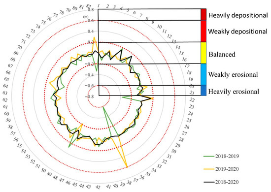
Figure 5.
Calculation results of the TCI (the differently coloured solid lines represent the results of the calculations for different years, and the red dashed lines are the standard lines for assessing the TCI strength levels).
Table 2.
TCI statistics.
7. Analysis and Discussion
7.1. Analysis of Balanced Points
The TCI was assessed, and the effect of the wind turbine on the topography was mainly balanced (95.12%). A balanced effect means that the wind turbine’s impact on the topography is within the acceptable range, but it still has some deposition on or erosion of the topography. In the two-year period of 2018–2020, continuous erosional/depositional conditions, or the opposite, may occur. Therefore, the erosion and deposition of wind turbines at the balance point in the first and second years (i.e., positive and negative TCRs) were counted, and the continuous impact was statistically analysed. The results revealed 11 enhanced deposition points, 12 enhanced erosion points and 56 opposite deposition/erosion points (Figure 6), and the opposite deposition/erosion points reached 71.79%. This suggests that the impact of wind turbines on OIS topography may show an oscillatory decrease over time since construction. In the future, we expect to conduct continuous monitoring for a longer period. In addition, the number of these wind turbines in stable or unstable areas and the average level of impact were counted. Over 2018–2020, 21 wind turbines in the stable zone caused an average erosion/deposition of only 2.32 cm, while the other 57 turbines in the unstable zone caused an average erosion/deposition of 3.09 cm. The wind turbine in the stable area caused approximately 25% less erosion/deposition than in the unstable area. This has implications for wind turbine site selection, and more stable areas should be selected for wind turbine construction.
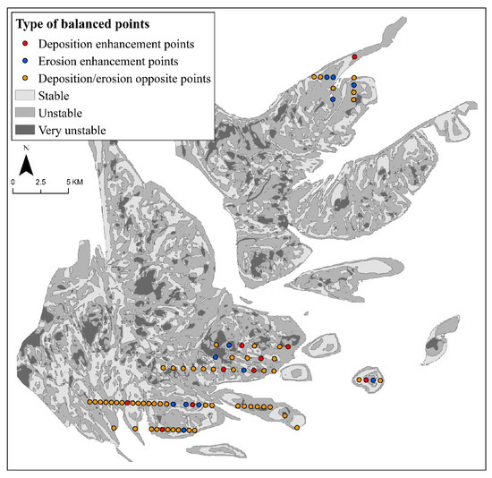
Figure 6.
Classification results for the impact of persistent siltation at the balance points (the differently coloured points represent the types of balanced points; the colour of the study area represents the stability of the topography).
To further understand the effect of the wind turbine on natural flushing, the TCI of the balanced turbine is compared with the change in the HSSE, i.e., natural flushing. If the natural erosional/depositional situation is erosional and the TCI is also erosional, then the turbine enhances natural erosion; if the TCI is depositional, it attenuates the effect of natural erosion. In the first year, 45 points strengthened the original erosional/depositional situation, with an average of 3.29 cm for erosion and 4.00 cm for deposition. The remaining 33 points caused the opposite absolute erosional/depositional depth of 3.85 cm on average. In the second year, there were small changes in the numbers, with changes of 27 and 51, respectively. Except for a small increase in the effect of enhanced deposition (4.15 cm), there was a small weakening of the effect of both enhanced erosion and the opposite, i.e., 2.10 cm and 3.00 cm, respectively. The change in the number and percentage suggest that wind turbines may have an enhancing effect on natural erosion/deposition, with more than 57% of wind turbines synchronized with natural erosional/depositional conditions in both years. The decrease in the value can indicate that as the time of wind turbine use increases, its influence on the topography becomes progressively smaller and gradually tends to be purely natural.
7.2. Analysis of Erosional/Depositional Points
For the calculated total of four affected erosional/depositional points (Figure 7), although they represent only 4.9% of the total number of points, these points can still reveal information. A comparison of these points in DEM and remote sensing images showed that the locations of these points were mainly at the edges of the topography or in the tidal channels, and three of them were located in unstable areas. The study area has a high number of tidal channels, while the oscillation of tidal channels is obvious due to the influence of hydrodynamic and depositional environments. The construction of wind turbines in these places with large topographic variations may cause nonbalanced types of erosion or deposition. The same is true for wind turbines at the edges of the topography, which are subject to change due to multiple factors because they are near the land–sea interface. The construction of wind turbines may lead to changes in the original environmental system and cause some erosion or deposition. Therefore, to avoid possible effects, wind turbine construction should be avoided near the edges of tidal channels and tidal flats.
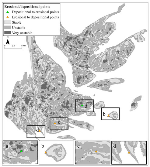
Figure 7.
Distribution of erosional/depositional points (the differently coloured triangles represent erosional/depositional points) ((a–d) are the specific locations of the points).
7.3. Comparison with Results from Semitheoretical Formulas
Currently, semitheoretical formulas are commonly used for estimating the final washout appearance caused by the construction of offshore wind turbines. Therefore, the reliability of the TCR was compared via the results obtained from the calculation. The calculation takes into account the interconnection of factors, such as sediment and water flow, and provides a theoretical basis for the construction of offshore wind farms.
Under the flow field conditions and the average action of the diurnal spring tide, the depth of erosion or deposition per unit area over ∆t time was obtained according to the equation for riverbed deformation (Equation (3)). is the thickness of erosion or deposition, is the dry density of bed sediment, is the sediment concentration of the water body, is the sedimentation rate, is the sedimentation speed, and is the sediment carrying capacity of the tide.
Under the assumption that the sediment particle size is unchanged before and after the construction of the wind turbine, the sediment carrying capacity can be calculated by using the Liujiaju equation for the sediment concentration and the sediment carrying capacity of silt and other sediments, and the equilibrium thickness of erosion or deposition is obtained by substituting it into Equation (3) (Equation (4)).
where and are the corresponding flow velocities before and after the construction of the wind turbine considering the tidal current, drift current and wave current, respectively. and are the water depths before and after the construction of the wind turbine, respectively. The relationship between the thickness of erosion or deposition and water depth is , which is substituted into Equation (4); when , the equilibrium thickness of erosion or deposition is obtained as follows:
where . The data of other parameters are obtained and substituted into Equation (5) to calculate the first year and equilibrium thickness of erosion or deposition at the point before and after the completion of the wind turbine.
The average first-year thickness of erosion or deposition at the points before and after the completion of the wind turbine was calculated as no more than 0.30 m, and the average thickness of erosion or deposition is no more than 0.02 m. By comparing seven points (Figure 8), the thickness of erosion or deposition obtained by using the HSSDM in this paper is greater than that estimated by the formula, and the difference is an average of 0.10 m. Although the semitheoretical formulas take into account various environmental factors, the variability in tidal channels is a factor that cannot be ignored in the study area. As the tide rises and falls, the tidal channels in the study area evolve, and this evolution is currently more difficult to calculate via the model, so the calculation results may be relatively small.
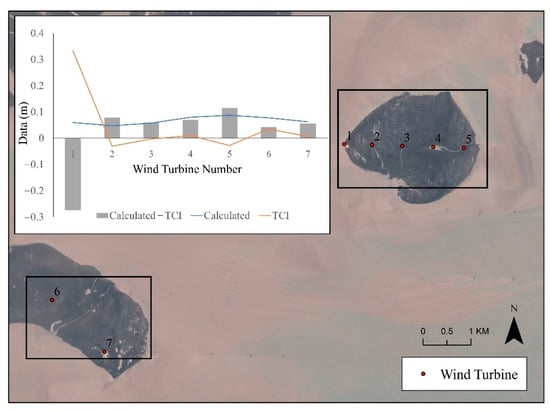
Figure 8.
Comparison with the results calculated by semitheoretical formulas.
8. Conclusions
First, the refined tidal topography for 2018–2020 was constructed by improving the waterline method. Then, the TCI caused by wind turbine construction was quantitatively analysed based on the HSSDM, and the possible influence of topographic stability on the TCI in the study area was analysed.
Based on the constructed DEM of the study area from 2018 to 2020, more than 90% of the wind turbines had a balanced impact on the erosion and deposition of the topography by the TCR in each year. The erosional or depositional points are the same in all years, with opposite erosional or depositional impacts, resulting in the final overall balanced impact in 2018–2020.
By combining the locations of the stable or unstable zones in which the wind turbines are located, it was found that the wind turbines in the stable zone caused approximately 25% less erosion or deposition than those in the unstable zone and that three of the four wind turbines that caused erosion or deposition were located in the unstable zone. The TCI is similar to the results obtained from the semitheoretical equations. The above results show that wind turbine construction has less influence on the erosion and deposition of the topography and provides some help for the site selection of wind turbine construction and monitoring of the wind turbine after completion.
Author Contributions
Conceptualization, H.Z. and D.Z.; methodology, H.Z., D.Z. and M.E.J.C.; validation, H.Z., and Y.Z.; formal analysis, H.Z.; resources, D.Z. and Z.Z.; data curation, H.Z. and Y.Z.; writing—original draft preparation, H.Z.; writing—review and editing, D.Z. and M.E.J.C.; visualization, H.Z.; supervision, D.Z. and Z.Z.; project administration, D.Z. and D.C.; funding acquisition, D.C. All authors have read and agreed to the published version of the manuscript.
Funding
This research was funded by National Natural Science Foundation of China (No. 41771447 and No. 42171465) and Postgraduate Research & Practice Innovation Program of Jiangsu Province (No. 1812000024513).
Institutional Review Board Statement
Not applicable.
Informed Consent Statement
Not applicable.
Data Availability Statement
Not applicable.
Conflicts of Interest
The authors declare no conflict of interest.
References
- Pechak, O.; Mavrotas, G.; Diakoulaki, D. Role and contribution of the clean development mechanism to the development of wind energy. Renew. Sustain. Energy Rev. 2011, 15, 3380–3387. [Google Scholar] [CrossRef]
- Zou, C.; Xiong, B.; Xue, H.; Zheng, D.; Ge, Z.; Wang, Y.; Jiang, L.; Pan, S.; Wu, S. The role of new energy in carbon neutral. Pet. Explor. Dev. 2021, 48, 411–420. [Google Scholar] [CrossRef]
- Xu, L.; Li, F.; Peng, H. Development of offshore wind power and its environmental problems in China. China Popul. Resour. Environ. 2015, 25, 135–138. [Google Scholar]
- Jiang, D.; Zhuang, D.; Huang, Y.; Wang, J.; Fu, J. Evaluating the spatio-temporal variation of China’s offshore wind resources based on remotely sensed wind field data. Renew. Sustain. Energy Rev. 2013, 24, 142–148. [Google Scholar] [CrossRef]
- Olaniyi, A.O.; Abdullah, A.M.; Ramli, M.F.; Alias, M.S. Assessment of drivers of coastal land use change in Malaysia. Ocean. Coast. Manag. 2012, 67, 113–123. [Google Scholar] [CrossRef]
- Xie, W.; He, Q.; Zhang, D.; Zhu, L.; Guo, L.; Wang, X. The response of morphplogy and sediment characteristics to human modification in an estuarine tidal flat. Acta Oceanol. Sin. 2019, 41, 118–127. [Google Scholar]
- Wang, Y.P.; Gao, S.; Jia, J.; Thompson, C.; Gao, J.; Yang, Y. Sediment transport over an accretional intertidal flat with influences of reclamation, Jiangsu coast, China. Mar. Geol. 2012, 291–294, 147–161. [Google Scholar] [CrossRef]
- Chen, W.; Zhang, D.; Cui, D.; Lv, L.; Xie, W.; Shi, S.; Hou, Z. Monitoring spatial and temporal changes in the continental coastline and the intertidal zone in Jiangsu province, China. Acta Geogr. Sin. 2018, 73, 1365–1380. [Google Scholar]
- Chen, Y.; Liu, H.Z.; Xiang, Y.; Cheng, T. Numerical Simulation of Wind Energy Characteristics in Jiangsu Coastal Area. Adv. Mater. Res. 2012, 347–353, 2156–2159. [Google Scholar] [CrossRef]
- Qi, C.; Liao, Q.; Dong, H.; Yang, J.; Li, J. Analysis of the impact of wind farm in inter-tidal zone on marine hydrodynamic field of radial sandy ridge in Jiangsu. Environ. Pollut. Control 2011, 33, 69–80. [Google Scholar]
- Wilhelmsson, D.; Malm, T.; Öhman, M.C. The influence of offshore windpower on demersal fish. ICES J. Mar. Sci. 2006, 63, 775–784. [Google Scholar] [CrossRef] [Green Version]
- Su, W.; Wu, N.; Zhang, L.; Chen, M. A review of research on the effect of offshore wind power project on marine organisms. Mar. Sci. Bull. 2020, 39, 291–299. [Google Scholar]
- Tup, A.; Bms, B.; Jf, B.; Tcr, C.; Jjs, C. Edge scour at scour protections around piles in the marine environment—Laboratory and field investigation—ScienceDirect. Coast. Eng. 2015, 106, 42–72. [Google Scholar]
- Zhou, Y.; Ning, D.; Shi, W.; Johanning, L.; Liang, D. Hydrodynamic investigation on an OWC wave energy converter integrated into an OWT monopile. Coast. Eng. 2020, 162, 103731. [Google Scholar] [CrossRef]
- Wu, X.; Hu, Y.; Li, Y.; Yang, J.; Duan, L.; Wang, T.G.U.; Adcock, T.; Jiang, Z.; Gao, Z.; Lin, Z. Foundations of offshore wind turbines: A review. Renew. Sustain. Energy Rev. 2019, 104, 379–393. [Google Scholar] [CrossRef] [Green Version]
- Harris, J.M.; Whitehouse, R. Scour Development around Large-Diameter Monopiles in Cohesive Soils: Evidence from the Field. J. Waterw. Port Coast. Ocean. Eng. 2017, 143, 4017022. [Google Scholar] [CrossRef] [Green Version]
- Qi, W.G.; Gao, F.P. Physical modeling of local scour development around a large-diameter monopile in combined waves and current. Coast. Eng. 2014, 83, 72–81. [Google Scholar] [CrossRef] [Green Version]
- Kusiak, A.; Zheng, H.; Zhe, S. Wind farm power prediction: A data-mining approach. Wind Energy 2010, 12, 275–293. [Google Scholar] [CrossRef]
- Mccombs, M.P.; Mulligan, R.P.; Boegman, L. Offshore wind farm impacts on surface waves and circulation in Eastern Lake Ontario. Coast. Eng. 2014, 93, 32–39. [Google Scholar] [CrossRef]
- Matutano, C.; Negro, V.; Lopez-Gutierrez, J.S.; Esteban, M.D. Scour prediction and scour protections in offshore wind farms. Renew. Energy 2013, 57, 358–365. [Google Scholar] [CrossRef] [Green Version]
- Choi, J.K.; Ryu, J.H.; Lee, Y.K.; Yoo, H.R.; Han, J.W.; Chang, H.K. Quantitative estimation of intertidal sediment characteristics using remote sensing and GIS. Estuar. Coast. Shelf Sci. 2010, 88, 125–134. [Google Scholar] [CrossRef]
- Salameh, E.; Frappart, F.; Almar, R.; Baptista, P.; Heygster, G.; Lubac, B.; Raucoules, D.; Almeida, L.P.; Bergsma, E.W.J.; Capo, S.; et al. Monitoring Beach Topography and Nearshore Bathymetry Using Spaceborne Remote Sensing: A Review. Remote Sens. 2019, 11, 2212. [Google Scholar] [CrossRef] [Green Version]
- Guo, L.; Brand, M.; Sanders, B.F.; Foufoula-Georgiou, E.; Stein, E.D. Tidal asymmetry and residual sediment transport in a short tidal basin under sea level rise. Adv. Water Resour. 2018, 121, 1–8. [Google Scholar] [CrossRef]
- Ryu, J.H.; Kim, C.H.; Lee, Y.K.; Won, J.S.; Chun, S.S.; Lee, S. Detecting the intertidal morphologic change using satellite data. Estuar. Coast. Shelf Sci. 2008, 78, 623–632. [Google Scholar] [CrossRef]
- Zhang, Y.; Zhang, Y.; Zhang, D.; Qian, Y. An underwater bathymetry reversion in the radial sand ridge group region of the southern Huanghai Sea using the remote sensing technology. Acta Oceanol. Sin. 2009, 31, 39–45. [Google Scholar]
- Kang, Y.; Ding, X.; Xu, F.; Zhang, C.; Ge, X. Topographic mapping on large-scale tidal flats with an iterative approach on the waterline method. Estuar. Coast. Shelf Sci. 2017, 190, 11–22. [Google Scholar] [CrossRef]
- Wang, Y.; Liu, Y.; Jin, S.; Sun, C.; Wei, X. Evolution of the topography of tidal flats and sandbanks along the Jiangsu coast from 1973 to 2016 observed from satellites. ISPRS J. Photogramm. Remote Sens. 2019, 150, 27–43. [Google Scholar] [CrossRef]
- Mason, D.C.; Davenport, I.J.; Flather, R.A.; Gurney, C. Cover A digital elevation model of the inter-tidal areas of the Wash, England, produced by the waterline method. Int. J. Remote Sens. 1998, 19, 1455–1460. [Google Scholar] [CrossRef]
- Zheng, Z.; Zhou, Y.; Jiang, X.; Shen, F. Waterline extraction and DEM reconstruction in Chongming Dongtan. Remote Sens. Technol. Appl. 2007, 22, 5. [Google Scholar]
- Li, N.; Niu, S.; Guo, Z.; Wu, L.; Zhao, J.; Min, L.; Ge, D.; Chen, J. Dynamic Waterline Mapping of Inland Great Lakes Using Time-Series SAR Data From GF-3 and S-1A Satellites: A Case Study of DJK Reservoir, China. IEEE J. Sel. Top. Appl. Earth Obs. Remote Sens. 2019, 12, 4297–4314. [Google Scholar] [CrossRef]
- Sagar, S.; Roberts, D.; Bala, B.; Lymburner, L. Extracting the intertidal extent and topography of the Australian coastline from a 28 year time series of Landsat observations. Remote Sens. Environ. 2017, 195, 153–169. [Google Scholar] [CrossRef]
- Fei, X.; Wang, Y.P.; Wang, H.V. Tidal hydrodynamics and fine-grained sediment transport on the radial sand ridge system in the southern Yellow Sea. Mar. Geol. 2012, 291–294, 192–210. [Google Scholar]
- Ding, X.; Zhou, H.; Kang, Y. Geomorphologic structure analysis of radial sand ridges. Geogr. Geo-Inf. Sci. 2014, 30, 6. [Google Scholar]
- Huang, L.; Huang, Z. Tidal Theory and Calculation; China Ocean University Press: Qingdao, China, 2005. [Google Scholar]
- Huang, L.; Cao, J.; Zhang, K.; Fu, Y.; Xu, H. Status and Prospects on Operation and Maintenance of Offshore Wind Turbines. Proc. CSEE 2016, 36, 729–738. [Google Scholar]
- Zhou, Y.; Zhang, D.; Deng, H.; Xu, N.; Zhang, H.; Hao, X.; Shen, Y. The enhanced construction method for intertidal terrain of offshore sandbanks by remote sensing. Acta Oceanol. Sin. 2021, 43, 11. [Google Scholar]
Publisher’s Note: MDPI stays neutral with regard to jurisdictional claims in published maps and institutional affiliations. |
© 2022 by the authors. Licensee MDPI, Basel, Switzerland. This article is an open access article distributed under the terms and conditions of the Creative Commons Attribution (CC BY) license (https://creativecommons.org/licenses/by/4.0/).