Vertical Motion Control of an Underwater Glider with a Command Filtered Adaptive Algorithm

Abstract

Underwater gliders are widely used in oceanic observation, which are driven by a hydraulic buoyancy regulating system and a movable mass. Better motion performance can help us to accomplish observation tasks better. Therefore, a command filtered adaptive algorithm with a detailed system dynamic model is proposed for underwater gliders in this paper. The dynamic model considers seawater density variation, temperature variation and hull deformation according to dive depth. The hydraulic pump model and the movable mass dynamic are also taken into account. An adaptive nonlinear control strategy based on backstepping technique is developed to compensate the uncertainties and disturbances in the control system. To deal with the command saturation and calculation of derivatives in the backstepping process, command filtered method is employed. The stability of the whole system is proved through the Lyapunov theory. Comparative simulations are conducted to verify the effectiveness of the proposed controller. The results demonstrate that the proposed algorithm can improve the motion control performance for underwater gliders under uncertainties and disturbances.

1. Introduction

Underwater gliders are widely used in oceanic exploration, because of their long-range, low-energy consumption, and low-cost characteristics [1,2]. Underwater gliders are generally driven by a hydraulic buoyancy regulating system and a movable mass. The hydraulic buoyancy regulating system consists of a hydraulic pump, an inner bladder, an external bladder, and several hydraulic valves. Underwater gliders control the hydraulic oil volume in the external bladder to adjust the buoyancy. Meanwhile, underwater gliders regulate the posture through changing the linear position and rotation angle of the movable mass.

Accurate motion tracking control of underwater gliders is required to complete different oceanic survey tasks. Precise attitude and velocity of underwater gliders could help collect detailed data of desired profiles, such as thermocline [3,4]. In addition, virtual mooring is an effective way to extend the duration of underwater gliders [5,6], which makes long-term oceanic phenomenon monitoring possible.

As an accurate mathematical model makes high performance control much easier, it is necessary to take all important influences into consideration. Underwater gliders, especially deep-sea underwater gliders, suffer from pressure variation, seawater density variation, temperature variation and hull deformation. Wang et al. [7] obtained the net buoyancy of autonomous underwater gliders through combing finite element method and density change with the water depth. A nonlinear dynamic model considering seawater pressure, temperature, and density, and the deformation of the pressure hull of the underwater glider was proposed by Gao et al. [8]. Yang et al. [9] established a dynamic model for deep-sea hybrid-driven underwater gliders considering hull deformation and seawater density variation, and proposed a buoyancy compensation scheme. Wang et al. [10] presented a dual-buoyancy-driven mechanism for a full ocean depth glider, and derived a dynamic model considering the influences of environment. Zhou et al. [11] developed a mathematical model of deep-sea gliders with hybrid buoyancy regulating system, which took hull deformation and seawater density variation into consideration. Researchers have considered the essential factors that influence underwater gliders. However, established models are only used to derive the gliding states, which have not been applied in the motion control process. Therefore, it is important to design controllers for underwater gliders with the help of the established accurate models. In addition, to make a more reliable model, the dynamic of actuators, i.e., the hydraulic pump model and the movable mass dynamic, should be considered.

To improve the motion control performance of underwater gliders, many researchers have done lots of work. Leonard and Graver [12] derived a nonlinear dynamic model of a nominal glider, and designed a model-based LQR (linear quadratic regulator) to control the vertical motion. Abraham and Yi [13] presented a model predictive control (MPC) design for buoyancy propelled autonomous underwater glider to compensate disturbances, which was confirmed by comparison to the PID controller. Song et al. [14] developed a dynamic surface decoupling control (DSDC) algorithm based on the active disturbance rejection control (ADRC) for an underwater glider, which reduced overshoot and settling time. Zhou et al. [15] proposed designated area persistent monitoring strategies for hybrid underwater profilers, which was verified by simulations and sea trials. Adaptive robust sliding mode control of an underwater glider with input constraints for virtual mooring was proposed by Zhou et al. [16], which incorporated model uncertainties, environmental disturbances and limited dynamic range of actuators. Jeong et al. [17] applied the machine learning algorithm to the navigation of the underwater glider. Wang et al. [18] designed a vertical profile diving and floating motion controller for underwater gliders based on fuzzy adaptive LADRC algorithm, which allowed the glider to dive to a predetermined depth precisely or float at a specific depth.

However, it is still a great challenge to obtain high motion tracking performance of underwater gliders, due to the strong parametric uncertainties, model uncertainties and disturbances. Model compensation [19] based control is one of the most feasible approaches, which requires an accurate model to capture the system’s nonlinearities and uncertainties. Adaptive control [19,20,21,22,23,24,25,26] can improve control systems’ dynamic performance and static precision through online approximation and compensation. Sliding mode control [27,28,29] can compensate the model uncertainties and disturbances. In general, underwater gliders are driven by a hydraulic buoyancy regulating system and a movable mass. The motion dynamic of underwater gliders is low, which may cause command saturation in the backstepping process of controller design. Meanwhile, the calculation of derivatives must be taken into consideration, because of the existing model uncertainties and disturbances. Command filter [30,31] is an effective technique to deal with command saturation and calculation of derivatives in the backstepping process.

To achieve better motion control performance and maneuverability of underwater gliders, a detailed system dynamic model is developed for controller design and simulation. The model considers not only the environment influence, e.g., seawater density variation, temperature variation and hull deformation according to dive depth, but also the dynamic model of system actuators, i.e., the hydraulic pump model and the movable mass dynamic, which could provide a more accurate simulation model, and help obtain high control performance through model compensation. Command filtered method is synthesized with backstepping technique to handle the low dynamic of underwater gliders. Adaptive control is employed to compensate the uncertainties and disturbances in the system.

This paper is organized as follow. Firstly, a detailed nonlinear mathematical model of the underwater glider is derived. Secondly, a nonlinear adaptive controller based on command filtered algorithm and backstepping method is designed. Next, the stability of the overall control system is proved through Lyapunov theory. Finally, comparative simulations are conducted to verify the effectiveness of the proposed controller. In addition, the nomenclature of this paper is provided in the Nomenclature.

2. Problem Formulation

There are two main operation patterns of underwater gliders, i.e., zigzag motion and spiraling motion. Zigzag motion is in the vertical plane. Virtual mooring could be simplified into a first stage three-dimensional movement and a second stage vertical movement, to improve the reliability in the practice use. So, this paper focuses on the vertical motion control of underwater gliders. The velocity and its direction are of significant importance for high performance ocean exploration.

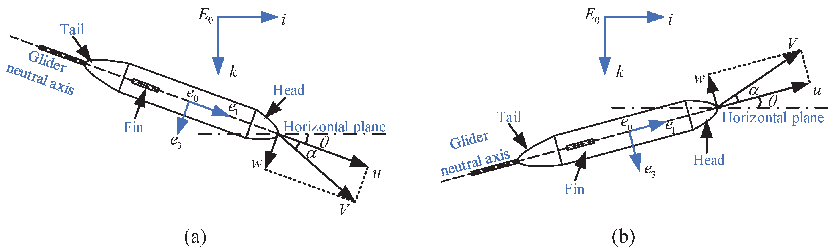
Inertial-referenced frame (IRF) $E_0$-$ik$ and body-referenced frame (BRF) $e_0$-$e_1{e}_3$ are always used to describe the motion of underwater vehicles. As shown in Figure 1, in IRF, the k-axis is oriented in the same direction as gravity; in BRF, the $e_1$-axis coincides with the longitudinal axis of the underwater glider, the $e_3$-axis is orthogonal to $e_1$-axis and pointing to the bottom. Motion equation of underwater gliders in the vertical plane could be obtained,

$$\begin{array}{c}\begin{array}{cc}& \dot{x}=ucos\theta +wsin\theta \hfill \\ & \dot{z}=-usin\theta +wcos\theta \hfill \\ & \dot{\theta }=q\hfill \end{array}\hfill \end{array}$$

(1)

where x, z are the position of the underwater glider in the vertical plane according to IRF, of which x denotes the horizontal movement distance and z denotes the dive depth. $\theta$ is the pitch angle, u and w are the velocity in BRF, q is the pitch angular velocity. The velocity and pitch angle of underwater gliders in vertical plane are shown in Figure 1.

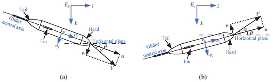
Figure 1. Velocity and pitch angle of underwater gliders in vertical plane. (a) Submerging process; (b) Floating process.

According to previous works [16], a decoupled motion dynamics of underwater gliders in the vertical plane can be developed,

$$\begin{array}{c}\begin{array}{cc}& \begin{array}{cc}\dot{q}=\hfill & \frac{1}{I_{f_2}}[\left(M_{f_3}-M_{f_1}+K_M\right)uw-\left(m_{b}g-\Delta B_e\right)r_{b}cos\theta \hfill \\ & -m_{p}g\left(r_{p}cos\theta +R_{p}sin\theta \right)+\left(K_{M_0}+K_{q}q\right)u^2+d_q]\hfill \end{array}\hfill \\ & \dot{u}=\frac{1}{M_{f_1}}\left[-K_{D_0}{u}^2+K_{L_0}uw+\Delta B_{b}sin\theta +d_u\right]\hfill \\ & \dot{w}=\frac{1}{M_{f_3}}\left[-K_{L_0}{u}^2-\left(K_L+K_{D_0}\right)uw-\Delta B_{b}cos\theta +d_w\right]\hfill \end{array}\hfill \end{array}\hfill$$

(2)

where $M_{f_1}$ and $M_{f_3}$ are the added mass, $I_{f_2}$ is the added moment of inertial, $K_M$, $K_{M_0}$, $K_q$, $K_{D_0}$, $K_L$ and $K_{L_0}$ are hydrodynamic coefficients of underwater gliders, $m_b$ is the change value of the oil mass in the external bladder, $m_p$ is the value of the movable mass, $r_b$ is the distance between the external bladder and the center of gravity (CG), $r_p$ is the distance between the movable mass and CG, $R_p$ is the rotational radius of the movable mass, $\Delta B_e$ is the buoyancy change value with respect to the hydraulic buoyancy regulating system, $\Delta B_b$ is the total change value of buoyancy, g is the gravitational acceleration, $d_q$, $d_u$ and $d_w$ are disturbances and lumped model uncertainties in the motion dynamics respectively.

The total change value of buoyancy could be described as

$$\begin{array}{c}\hfill \Delta B_b=\Delta B_e-\Delta B_h\end{array}$$

(3)

where $\Delta B_h$ is the buoyancy change value generated by the pressure hull of underwater gilders.

The hull volume will be compressed owing to the seawater pressure. The seawater density variation and the temperature variation also affect the buoyancy generated by pressure hull. The relationship can be expressed as

$$\begin{array}{c}\hfill \Delta B_h={\rho }_{sea}\left(z\right)V_{h0}\left[{\kappa }_t\left(T_0-T\left(z\right)\right)+{\kappa }_h{\rho }_{sea}\left(z\right)gz\right]\end{array}$$

(4)

where ${\rho }_{sea}\left(z\right)$ is the seawater density at the depth z, $V_{h0}$ is the volume of the pressure hull in the air, ${\kappa }_t$ and ${\kappa }_h$ are the influence coefficients of temperature and seawater pressure respectively, $T_0$ and $T\left(z\right)$ are temperatures of seawater at sea surface and depth z respectively, which are also can be measured by a temperature sensor.

According to previous works [11], the seawater density and temperature of South China Sea can be approximated as

$$\begin{array}{c}\hfill {\rho }_{sea}\left(z\right)={\rho }_{sea}\left(0\right)+1.7806ln\left(1+0.0478z\right)+0.0035z\end{array}$$

(5)

where ${\rho }_{sea}\left(0\right)$ is the seawater density at sea surface.

$$\begin{array}{c}\hfill T\left(z\right)=T_0/\left(az+1\right)\end{array}$$

(6)

where a is the coefficient of temperature variation.

The buoyancy produced by the hydraulic buoyancy regulating system can be written as

$$\begin{array}{c}\hfill \Delta B_e={\rho }_{sea}\left(z\right)g{V}_{oil}\end{array}$$

(7)

where $V_{oil}$ is the volume of the displaced hydraulic oil. $V_{oil}=\int Qdt$, which also can be measured by a cable linear displacement sensor. Q is the flow rate to the external bladder, t is the operating time of the pump.

Therefore, $m_b$ can be represented by $V_{oil}$

$$\begin{array}{c}\hfill m_b={\rho }_{oil}{V}_{oil}\end{array}$$

(8)

where ${\rho }_{oil}$ is the hydraulic oil density.

The dynamics of the hydraulic pump [10,32,33] is considered to provide a more accurate system model,

$$\begin{array}{c}\hfill Q=Dn-C_{t}P\left(z\right)\end{array}$$

(9)

where D is the displacement of the hydraulic pump, n is rational speed of the electrical motor, that drives the hydraulic pump. $C_t$ is the coefficient of the total internal leakage. $P\left(z\right)$ is the seawater pressure at depth z, and $P\left(z\right)={\rho }_{sea}\left(z\right)gz$, which also can be measured with a pressure sensor.

The dynamics of the electrical motor speed can be neglected, because the dynamics of the desired motion is significantly lower than the dynamics of the electrical motor. Therefore, it is assumed that the control voltage applied to the electrical motor is proportional to the rotational speed, as

$$\begin{array}{c}\hfill n={\kappa }_p{U}_1\end{array}$$

(10)

where ${\kappa }_p$ is a positive constant and $U_1$ is the control input voltage of the electrical motor.

However, the dynamics of the movable mass is not so high, which has to be considered,

$$\begin{array}{c}\hfill {\dot{r}}_p=-\frac{1}{{\tau }_{r_p}}{r}_p+\frac{{\kappa }_{r_p}}{{\tau }_{r_p}}{U}_2\end{array}$$

(11)

where ${\tau }_{r_p}$ and ${\kappa }_{r_p}$ are the time constant and the gain of the linear displacement dynamics of the movable mass respectively, $U_2$ is the control input voltage. In addition, $r_p$ can be measured with an encoder.

The following equilibrium equation of underwater gliders in the vertical plane [16] can be obtained,

$$\begin{array}{c}\begin{array}{cc}& \begin{array}{cc}{\alpha }_s=\hfill & \frac{1}{2}\left[-\frac{K_L}{K_D}tan{\xi }_s+\sqrt{{\left(\frac{K_L}{K_D}tan{\xi }_s\right)}^2-\frac{4}{K_D}\left(K_{D_0}+K_{L_0}tan{\xi }_s\right)}\right]\hfill \end{array}\hfill \\ & {\theta }_s={\xi }_s+{\alpha }_s\hfill \\ & u_s=V_{s}cos{\alpha }_s\hfill \\ & w_s=V_{s}sin{\alpha }_s\hfill \end{array}\hfill \end{array}$$

(12)

where s subindex stands for the equilibrium states, of which ${\alpha }_s$ is the attack angle, ${\xi }_s$ is the gliding angle, ${\theta }_s$ is the pitch angle, $u_s$ and $w_s$ are the velocity in BRF, $V_s$ is the velocity in IRF.

As ${\alpha }_s$ is usually very small [22], $w_s$ is very small compared to $u_s$. Therefore, only the velocity u and the pitch angle $\theta$ are taken in consideration of vertical plane motion control. It will not cause a big influence in a short time.

For simplification, define a set of parameters as $\eta$ $=[{\eta }_1,{\eta }_2,{\eta }_3,{\eta }_4,{\eta }_5,{\eta }_6]$, and ${\eta }_1=M_{f_3}-M_{f_1}+K_M$, ${\eta }_2=K_{M_0}$, ${\eta }_3=K_q$, ${\eta }_4=K_{D_0}$, ${\eta }_5=K_{L_0}$, ${\eta }_6=K_L+K_{D_0}$.

So, (2) can be expressed as

$$\begin{array}{c}\begin{array}{cc}& \begin{array}{c}\dot{q}=\frac{1}{I_{f_2}}\left[{\eta }_{1}uw+{\eta }_2{u}^2+{\eta }_{3}q{u}^2-\left(m_{b}g-\Delta B_e\right)r_{b}cos\theta -m_{p}g\left(r_{p}cos\theta +R_{p}sin\theta \right)+d_q\right]\hfill \end{array}\hfill \\ & \dot{u}=\frac{1}{M_{f_1}}\left[-{\eta }_4{u}^2+{\eta }_{5}uw+\Delta B_{b}sin\theta +d_u\right]\hfill \\ & \dot{w}=\frac{1}{M_{f_3}}\left[-{\eta }_5{u}^2-{\eta }_{6}uw-\Delta B_{b}cos\theta +d_w\right]\hfill \end{array}\hfill \end{array}$$

(13)

Remark 1.

For simplicity, assuming that the underwater glider initially has neutral buoyancy and balanced moment on the sea surface. The center of gravity (CG) in (2) means the initial center of gravity of the whole underwater gilder on the sea surface, which is considered unchangeable. In fact, the actual center of gravity may change, when the hydraulic pump and movable mass work. However, the correctness of (2) holds, no matter which rotational axis is chosen.

Remark 2.

$d_q$, $d_u$, $d_w$ are disturbances and lumped model uncertainties in the motion dynamics. The model uncertainties in the inner loops, such as $\Delta B_h$, $m_b$, are also considered in $d_q$, $d_u$, $d_w$.

Remark 3.

The dive depth z of the underwater glider can be measured by a depth gauge. Therefore, $\dot{z}$ can be calculated by differentiating z. The pitch angle θ could be measured with a gyroscope. However, the velocity u and w have to be measured with a DVL (Doppler velocity log).

3. Controller Design

The control objective is to make u and $\theta$ follow the desired velocity $u_d$ and pitch angle ${\theta }_d$ as close as possible, which could improve the operation performance in both vertical motion and virtual mooring. A command filtered adaptive algorithm based on backstepping procedure is proposed to compensate uncertainties and disturbances, and deal with the command saturation and calculation of derivatives.

Before the controller design, we have the following assumption.

Assumption 1.

The desired velocity $u_d$, pitch angle ${\theta }_d$ and their derivatives ${\dot{u}}_d$, ${\dot{\theta }}_d$, ${\ddot{\theta }}_d$ are bounded. Only the motion in vertical plane is considered in this paper. As the dynamics of the underwater glider is low, it is possible to design a smooth velocity and pitch angle command and keep their derivatives exist.

• Step 1:

This step concentrates on designing a desired buoyancy to make the velocity tracking error as small as possible, and designing an expected linear displacement of the movable mass to make the pitch angle tracking error as small as possible.

• Step 1.1:

Defining the velocity tracking error as

$$\begin{array}{c}\hfill \tilde{u}=u-u_d\end{array}$$

(14)

According to Assumption 1, differentiating (14) and noting (13),

$$\begin{array}{c}\begin{array}{cc}\dot{\tilde{u}}\hfill & =\dot{u}-{\dot{u}}_d\hfill \\ \hfill & =\frac{1}{M_{f_1}}\left[-{\eta }_4{u}^2+{\eta }_{5}uw+\Delta B_{e}sin\theta -\Delta B_{h}sin\theta +d_u\right]-{\dot{u}}_d\hfill \end{array}\hfill \end{array}$$

(15)

A virtual control input $\Delta B_e^0$ for $\Delta B_e$ is designed as

$$\begin{array}{c}\hfill \begin{array}{cc}\hfill \Delta B_e^0=& \hfill \frac{1}{sin\theta }\left[{\widehat{\eta }}_4{u}^2-{\widehat{\eta }}_{5}uw+\Delta B_{h}sin\theta -{\widehat{d}}_u+M_{f_1}\left({\dot{u}}_d-c_1\tilde{u}\right)\right]-{\chi }_2\hfill \end{array}\end{array}$$

(16)

where ${\widehat{\eta }}_4$, ${\widehat{\eta }}_5$ and ${\widehat{d}}_u$ are the estimations of ${\eta }_4$, ${\eta }_5$ and $d_u$, $c_1$ is a positive constant, ${\chi }_2$ is an extra corrector term, which will be designed later. ${\tilde{\eta }}_4$, ${\tilde{\eta }}_5$ and ${\tilde{d}}_u$ are the estimation errors, which are defined as ${\tilde{\eta }}_4={\eta }_4-{\widehat{\eta }}_4$, ${\tilde{\eta }}_5={\eta }_5-{\widehat{\eta }}_5$, ${\tilde{d}}_u=d_u-{\widehat{d}}_u$.

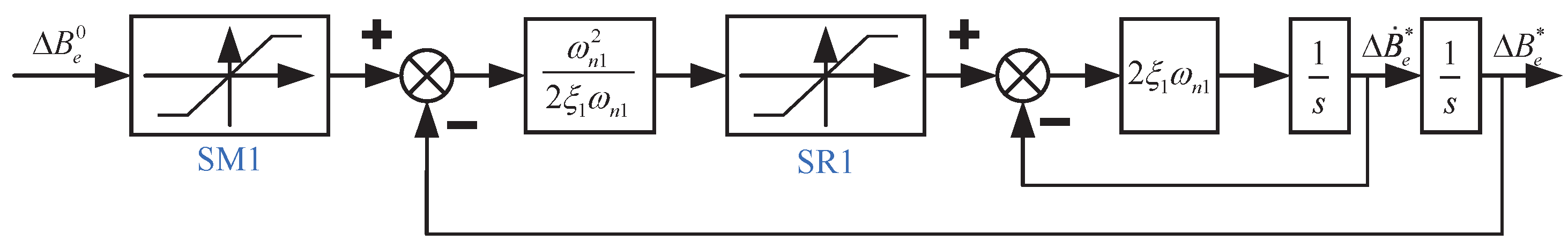
A second-order filter with coefficients ${\omega }_{n1}$ and ${\xi }_1$ showed in Figure 2 is applied on the virtual input $\Delta B_e^0$ to handle the command saturation and calculation of derivatives. The filtered output corresponding to $\Delta B_e^0$ is $\Delta B_e^{*}$.

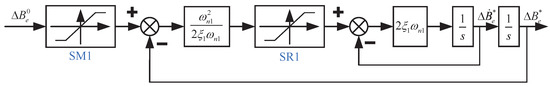
Figure 2. Schematic diagram of the command filter strategy applied on $\Delta B_e^0$.

The following errors are defined,

$$\begin{array}{c}\begin{array}{cc}\Delta {\tilde{B}}_e\hfill & =\Delta B_e-\Delta B_e^{*}\hfill \\ \Delta {\overline{B}}_e\hfill & =\Delta {\tilde{B}}_e-{\chi }_2\hfill \\ \hfill \overline{u}& =\tilde{u}-{\chi }_1\hfill \end{array}\hfill \end{array}$$

(17)

where ${\chi }_1$ is an extra corrector term, and is defined as ${\dot{\chi }}_1=-c_1{\chi }_1+\frac{sin\theta }{M_{f_1}}\left(\Delta B_e^{*}-\Delta B_e^0\right)$.

From (14) and (17), we can get

$$\begin{array}{c}\begin{array}{cc}\dot{\overline{u}}\hfill & =\dot{\tilde{u}}-{\dot{\chi }}_1=\dot{u}-{\dot{u}}_d-{\dot{\chi }}_1\hfill \\ & =\frac{1}{M_{f_1}}\left[-{\tilde{\eta }}_4{u}^2+{\tilde{\eta }}_{5}uw+{\tilde{d}}_u\right]-c_1\overline{u}+\frac{sin\theta }{M_{f_1}}\Delta {\overline{B}}_e\hfill \end{array}\hfill \end{array}$$

(18)

Define a following Lyapunov function

$$\begin{array}{c}\hfill V_1=\frac{1}{2}{k}_{11}{\overline{u}}^2+\frac{1}{2}{k}_{12}{\tilde{\eta }}_4^2+\frac{1}{2}{k}_{13}{\tilde{\eta }}_5^2+\frac{1}{2}{k}_{14}{\tilde{d}}_u^2\end{array}$$

(19)

where $k_{11}$, $k_{12}$, $k_{13}$ and $k_{14}$ are positive constants.

The adaption law is chosen as

$$\begin{array}{c}\begin{array}{cc}{\dot{\widehat{\eta }}}_4\hfill & =\frac{-k_{11}}{M_{f_1}{k}_{12}}{u}^2\overline{u}\hfill \\ {\dot{\widehat{\eta }}}_5\hfill & =\frac{k_{11}}{M_{f_1}{k}_{13}}uw\overline{u}\hfill \\ {\dot{\widehat{d}}}_u\hfill & =\frac{k_{11}}{M_{f_1}{k}_{14}}\overline{u}\hfill \end{array}\hfill \end{array}$$

(20)

Based on (18) and (20), the time derivative of $V_1$ is

$$\begin{array}{c}\hfill {\dot{V}}_1=-c_1{k}_{11}{\overline{u}}^2+\frac{k_{11}}{M_{f_1}}\overline{u}\Delta {\overline{B}}_{e}sin\theta \end{array}$$

(21)

• Step 1.2:

Meanwhile, define the pitch angle tracking error as

$$\begin{array}{c}\hfill \tilde{\theta }=\theta -{\theta }_d\end{array}$$

(22)

A sliding surface s is designed as

$$\begin{array}{c}\hfill s=\dot{\tilde{\theta }}+\lambda \tilde{\theta }\end{array}$$

(23)

where $\lambda$ is a positive constant. Since making $\tilde{\theta }$ small or converge to zero is equivalent to making s small or converge to zero, the rest of the design will focus on making s as small as possible.

According to Assumption 1, differentiating (23) and noting (13), (22), yielding the dynamics of s,

$$\begin{array}{c}\begin{array}{cc}\dot{s}\hfill & =\ddot{\tilde{\theta }}+\lambda \dot{\tilde{\theta }}\hfill \\ \hfill & =\frac{1}{I_{f_2}}[{\eta }_{1}uw+{\eta }_2{u}^2+{\eta }_{3}q{u}^2-\left(m_{b}g-\Delta B_e\right)r_{b}cos\theta \hfill \\ & -m_{p}g\left(r_{p}cos\theta +R_{p}sin\theta \right)+d_q]+\lambda q-\lambda {\dot{\theta }}_d-{\ddot{\theta }}_d\hfill \end{array}\hfill \end{array}$$

(24)

A virtual control input $r_p^0$ for $r_p$ is designed as

$$\begin{array}{c}\begin{array}{cc}{r}_p^0=\hfill & \frac{1}{m_{p}gcos\theta }[{\widehat{\eta }}_{1}uw+{\widehat{\eta }}_2{u}^2+{\widehat{\eta }}_{3}q{u}^2-\left(m_{b}g-\Delta B_e\right)r_{b}cos\theta -m_{p}g{R}_{p}sin\theta +{\widehat{d}}_q\hfill \\ & +I_{f_2}\left(\lambda q-\lambda {\dot{\theta }}_d-{\ddot{\theta }}_d-c_{3}s\right)]-{\chi }_4\hfill \end{array}\hfill \end{array}$$

(25)

where ${\widehat{\eta }}_1$, ${\widehat{\eta }}_2$, ${\widehat{\eta }}_3$ and ${\widehat{d}}_q$ are the estimations of ${\eta }_1$, ${\eta }_2$, ${\eta }_3$ and $d_q$, $c_3$ is a positive constant, ${\chi }_4$ is an extra corrector term, which will be designed later. ${\tilde{\eta }}_1$, ${\tilde{\eta }}_2$, ${\tilde{\eta }}_3$ and ${\tilde{d}}_q$ are the estimation errors, which are defined as ${\tilde{\eta }}_1={\eta }_1-{\widehat{\eta }}_1$, ${\tilde{\eta }}_2={\eta }_2-{\widehat{\eta }}_2$, ${\tilde{\eta }}_3={\eta }_3-{\widehat{\eta }}_3$, ${\tilde{d}}_q=d_q-{\widehat{d}}_q$.

A filter with same structure showed in Figure 2 but different parameters ${\omega }_{n2}$ and ${\xi }_2$, is applied on the virtual input $r_p^0$. In addition, $r_p^{*}$ is the filtered output.

Define the following errors

$$\begin{array}{c}\begin{array}{cc}\overline{s}\hfill & =s-{\chi }_3\hfill \\ {\tilde{r}}_p\hfill & =r_p-r_p^{*}\hfill \\ {\overline{r}}_p\hfill & ={\tilde{r}}_p-{\chi }_4\hfill \end{array}\hfill \end{array}$$

(26)

where ${\chi }_3$ is an extra corrector term, and is defined as ${\dot{\chi }}_3=-c_3{\chi }_3-\frac{1}{I_{f_2}}{m}_{p}gcos\theta \left(r_p^{*}-r_p^0\right)$.

Combing (24) and (26) yields

$$\begin{array}{c}\begin{array}{cc}\dot{\overline{s}}\hfill & =\dot{s}-{\dot{\chi }}_3\hfill \\ & \hfill =\frac{1}{I_{f_2}}\left[{\tilde{\eta }}_{1}uw+{\tilde{\eta }}_2{u}^2+{\tilde{\eta }}_{3}q{u}^2+{\tilde{d}}_q\right]-c_3\overline{s}-\frac{1}{I_{f_2}}{m}_{p}g{\overline{r}}_{p}cos\theta \hfill \end{array}\hfill \end{array}$$

(27)

Define a following Lyapunov function

$$\begin{array}{c}\hfill V_3=\frac{1}{2}{k}_{31}{\overline{s}}^2+\frac{1}{2}{k}_{32}{\tilde{\eta }}_1^2+\frac{1}{2}{k}_{33}{\tilde{\eta }}_2^2+\frac{1}{2}{k}_{34}{\tilde{\eta }}_3^2+\frac{1}{2}{k}_{35}{\tilde{d}}_q^2\end{array}$$

(28)

where $k_{31}$, $k_{32}$, $k_{33}$, $k_{34}$ and $k_{35}$ are positive constants.

A following adaption law is designed

$$\begin{array}{c}\hfill \begin{array}{cc}\hfill {\dot{\widehat{\eta }}}_1=& \hfill \frac{k_{31}}{I_{f_2}{k}_{32}}uw\overline{s}\hfill \\ \hfill {\dot{\widehat{\eta }}}_2=& \hfill \frac{k_{31}}{I_{f_2}{k}_{33}}{u}^2\overline{s}\hfill \\ \hfill {\dot{\widehat{\eta }}}_3=& \hfill \frac{k_{31}}{I_{f_2}{k}_{34}}q{u}^2\overline{s}\hfill \\ \hfill {\dot{\widehat{d}}}_q=& \hfill \frac{k_{31}}{I_{f_2}{k}_{35}}\overline{s}\hfill \end{array}\end{array}$$

(29)

Considering (27) and (29), the time derivative of $V_3$ can be calculated as

$$\begin{array}{c}\hfill {\dot{V}}_3=-c_3{k}_{31}{\overline{s}}^2-\frac{k_{31}}{I_{f_2}}{m}_{p}g\overline{s}{\overline{r}}_{p}cos\theta \end{array}$$

(30)

• Step 2:

This step focuses on the control inputs of the inner loop, which designs the control inputs of the electrical motor and movable mass.

• Step 2.1:

According to (7) and (17), we can get

$$\begin{array}{c}\begin{array}{cc}\Delta {\dot{\tilde{B}}}_e\hfill & =\Delta {\dot{B}}_e-\Delta {\dot{B}}_e^{*}\hfill \\ & ={\rho }_{sea}\left(z\right)g{\dot{V}}_{oil}-\Delta {\dot{B}}_e^{*}\hfill \\ & ={\rho }_{sea}\left(z\right)gQ-\Delta {\dot{B}}_e^{*}\hfill \end{array}\hfill \end{array}$$

(31)

So, the desired input $Q^0$ can be determined as

$$\begin{array}{c}\hfill Q^0=\frac{1}{{\rho }_{sea}\left(z\right)g}\left[\Delta {\dot{B}}_e^{*}-c_2\Delta {\tilde{B}}_e-\frac{k_{11}}{M_{f_1}{k}_2}\overline{u}sin\theta \right]\end{array}$$

(32)

And, the extra term ${\chi }_2$ is designed as

$$\begin{array}{c}\hfill {\dot{\chi }}_2=-c_2{\chi }_2+{\rho }_{sea}\left(z\right)g\left(Q-Q^0\right)\end{array}$$

(33)

where $c_2$ is a positive constant. In addition, Q is determined by applying a similar filter with coefficients ${\omega }_{n3}$ and ${\xi }_3$ showed in Figure 2 on $Q^0$.

Therefore, we can get

$$\begin{array}{c}\hfill \Delta {\dot{\overline{B}}}_e=\Delta {\dot{\tilde{B}}}_e-{\dot{\chi }}_2=-c_2\Delta {\overline{B}}_e-\frac{k_{11}}{M_{f_1}{k}_2}\overline{u}sin\theta \end{array}$$

(34)

Define a following Lyapunov function

$$\begin{array}{c}\hfill V_2=V_1+\frac{1}{2}{k}_2\Delta {\overline{B}}_e^2\end{array}$$

(35)

where $k_2$ is a positive constant.

Taking (21) and (34) into consideration, the time derivative of $V_2$ is given by

$$\begin{array}{c}\hfill {\dot{V}}_2=-c_1{k}_{11}{\overline{u}}^2-c_2{k}_2\Delta {\overline{B}}_e^2\end{array}$$

(36)

In addition, based on (9), (10), the control input of the electric motor could be determined as

$$\begin{array}{c}\hfill U_1=\frac{1}{D{\kappa }_p}\left[Q+C_t{\rho }_{sea}\left(z\right)gz\right]\end{array}$$

(37)

• Step 2.2:

According to (11) and (26), the dynamics of ${\dot{\tilde{r}}}_p$ can be expressed as

$$\begin{array}{c}\begin{array}{cc}{\dot{\tilde{r}}}_p\hfill & ={\dot{r}}_p-{\dot{r}}_p^{*}\hfill \\ & =-\frac{1}{{\tau }_{rp}}{r}_p+\frac{{\kappa }_{r_p}}{{\tau }_{rp}}{U}_2-{\dot{r}}_p^{*}\hfill \end{array}\hfill \end{array}$$

(38)

Thus, the desired input $U_2^0$ can be designed as

$$\begin{array}{c}\hfill U_2^0=\frac{{\tau }_{rp}}{{\kappa }_{r_p}}\left(\frac{1}{{\tau }_{rp}}{r}_p+{\dot{r}}_p^{*}-c_4{\tilde{r}}_p+\frac{k_{31}}{I_{f_2}{k}_4}{m}_{p}g\overline{s}cos\theta \right)\end{array}$$

(39)

The extra term ${\chi }_4$ could be also decided as

$$\begin{array}{c}\hfill {\dot{\chi }}_4=-c_4{\chi }_4+\frac{{\kappa }_{r_p}}{{\tau }_{rp}}\left(U_2-U_2^0\right)\end{array}$$

(40)

where $c_4$ is a positive constant. In addition, $U_2$ is determined by applying a similar filter with coefficients ${\omega }_{n4}$ and ${\xi }_4$ showed in Figure 2 on $U_2^0$.

So, the time derivative of ${\overline{r}}_p$ can be calculated

$$\begin{array}{c}\begin{array}{cc}{\dot{\overline{r}}}_p\hfill & ={\dot{\tilde{r}}}_p-{\dot{\chi }}_4\hfill \\ & =-c_4{\overline{r}}_p+\frac{k_{31}}{I_{f_2}{k}_4}{m}_{p}g\overline{s}cos\theta \hfill \end{array}\hfill \end{array}$$

(41)

Define a following Lyapunov function

$$\begin{array}{c}\hfill V_4=V_3+\frac{1}{2}{k}_4{\overline{r}}_p^2\end{array}$$

(42)

where $k_4$ is a positive constant.

Considering (30) and (41), the time derivative of $V_4$ is given by

$$\begin{array}{c}\hfill {\dot{V}}_4=-c_3{k}_{31}{\overline{s}}^2-c_4{k}_4{\overline{r}}_p^2\end{array}$$

(43)

Finally, define a following Lyapunov function

$$\begin{array}{c}\hfill V=V_2+V_4\end{array}$$

(44)

Combing (36) and (43), it could be easily obtained

$$\begin{array}{c}\hfill \dot{V}=-c_1{k}_{11}{\overline{u}}^2-c_2{k}_2\Delta {\overline{B}}_e^2-c_3{k}_{31}{\overline{s}}^2-c_4{k}_4{\overline{r}}_p^2\end{array}$$

(45)

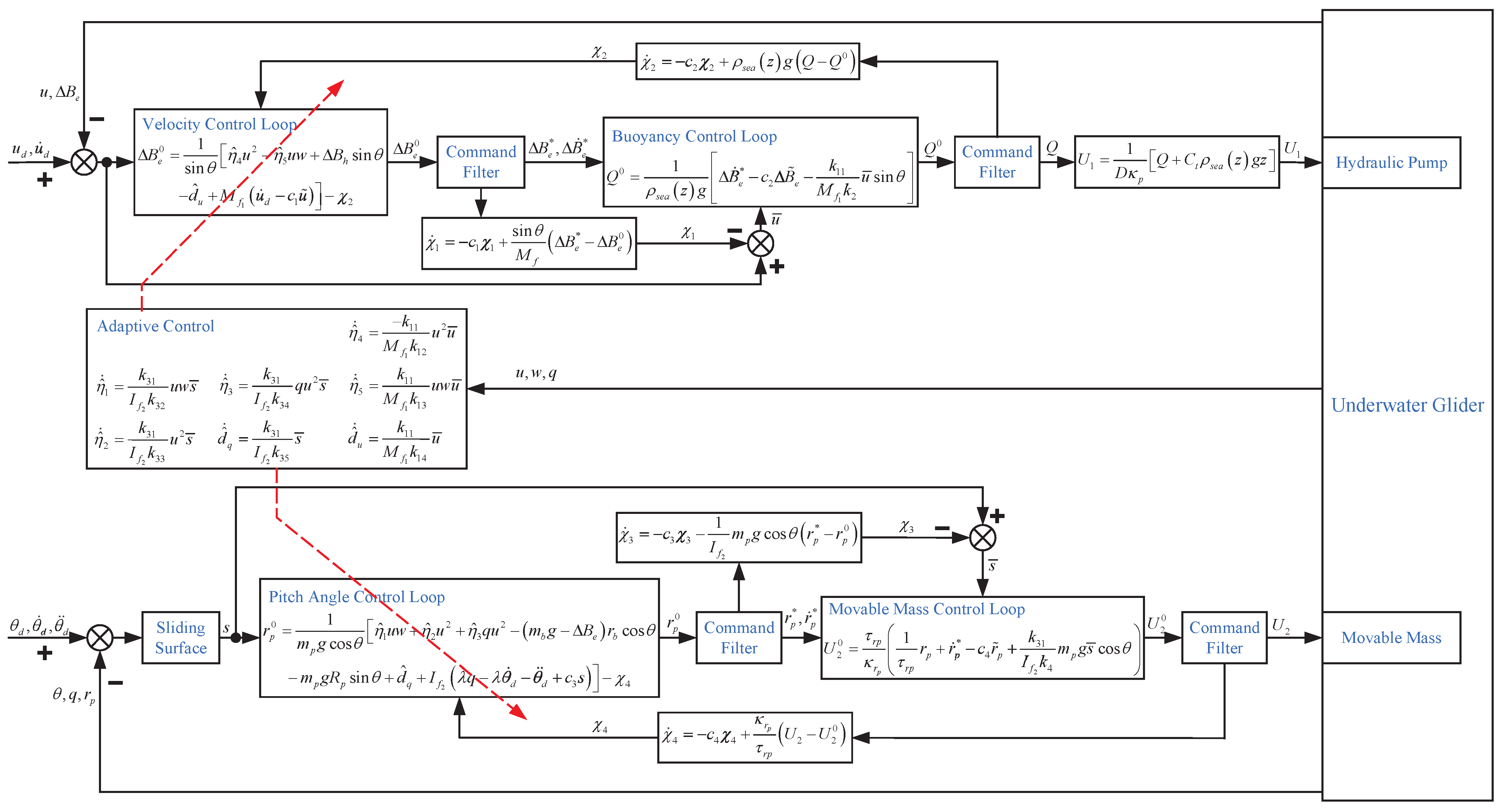
Therefore, $\dot{V}\le 0$, the stability of the control system has been proved. Figure 3 demonstrates the schematic diagram of the proposed command filtered adaptive control (CFAC) algorithm for underwater gliders.

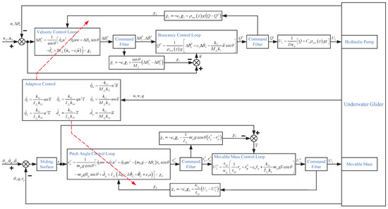
Figure 3. Schematic diagram of the proposed CFAC strategy.

Remark 4.

Extra corrector terms ${\chi }_1$, ${\chi }_2$, ${\chi }_3$, ${\chi }_4$ are the differences between the expected system errors and redefined errors with command filters, i.e., ${\chi }_1=\tilde{u}-\overline{u}$, ${\chi }_2=\Delta {\tilde{B}}_e-\Delta {\overline{B}}_e$, ${\chi }_3=s-\overline{s}$, ${\chi }_4={\tilde{r}}_p-{\overline{r}}_p$. ${\chi }_i$ ($i=1,2,3,4$) is defined as the first-order filter output of the command filter error. The design process is based on Lyapunov functions, which should make the differentiations of Lyapunov functions negative definite.

Remark 5.

The parameters in Lyapunov functions, i.e., $k_{11}$, $k_{12}$, $k_{13}$, $k_{14}$, $k_2$, $k_{31}$, $k_{32}$, $k_{33}$, $k_{34}$, $k_{35}$ and $k_4$ decide the convergence rate of the corresponding error. Their values should be determined based on simulation results.

4. Simulation and Discussion

Simulations based on three controllers are conducted to verify the effectiveness of the developed control strategy. The first was the proportional-integral-differential controller (PID), i.e., $U_1=sgn\left(u_d\right)(K_{P1}\tilde{u}+K_{I1}\int \tilde{u}dt+K_{D1}\frac{d\tilde{u}}{dt})$, $U_2=K_{P2}\tilde{\theta }+K_{I2}\int \tilde{\theta }dt+K_{D1}\frac{d\tilde{\theta }}{dt}$, where $sgn(•)$ is the signum function. The second was the nonlinear controller without parameter adaption and command filter (NC), i.e., $k_{11}=0$, $k_{31}=0$, $\Delta B_e^{*}=\Delta B_e^0$, $r_p^{*}=r_p^0$, $Q=Q^0$, $U_2=U_2^0$, and ${\chi }_1=0$, ${\chi }_2=0$, ${\chi }_3=0$, ${\chi }_4=0$. The third was the proposed CFAC strategy. The parameters of the underwater glider and seawater used for controller design and simulation are shown in Table 1. The control parameters of the aforementioned controllers are listed in Table 2 and Table 3 respectively. The simulations are implemented in MATLAB Simulink with a control rate of 100 Hz.

Table 1. Parameters of the underwater glider and seawater.

Parameter	Value	Unit
$m_p$	11	kg
g	$9.8$	m/s${}^2$
$r_b$	$0.075$	m
$r_p$	$[-0.05,0.05]$	m
$R_p$	$0.014$	m
${\rho }_{sea}\left(0\right)$	$1021.7$	kg/m${}^3$
$T_0$	30	${}^{\circ }$C
a	$0.0042$	m${}^{-1}$
$V_{h0}$	$0.06523$	m${}^3$
$V_{oil}$	$[-500,500]$	mL
${\kappa }_t$	$2.31\times {10}^{-6}$	(${}^{\circ }$C)${}^{-1}$
${\kappa }_h$	$1.46\times {10}^{-10}$	m${}^2$/kg
D	$4.5\times {10}^{-8}$	m${}^3$/r
$C_t$	$4\times {10}^{-15}$	m${}^3$/(s · Pa)
${\kappa }_p$	5	r/(s · V)
${\tau }_{r_p}$	2	s
${\kappa }_{r_p}$	$0.005$	m/V
$M_{f1},M_{f3}$	$1.48,65.92$	kg
$I_{f2}$	$7.88$	kg · m${}^2$
$K_M,K_{M0}$	$-65.84,0.28$	kg
$K_q$	$-205.64$	kg · s
$K_{D0}$	$7.19$	kg/m
$K_L,K_{L0}$	$440.99,-0.36$	kg/m
$U_1$	$[-10,10]$	V
$U_2$	$[-10,10]$	V

Table 2. Parameters of CFAC.

Parameter	Value	Parameter	Value
$c_1$	5	$k_{33}$	$0.01$
$c_2$	$0.1$	$k_{34}$	$0.001$
$c_3$	$0.1$	$k_{35}$	$0.01$
$c_4$	$0.5$	$k_4$	100
$\lambda$	1	${\omega }_{n1}$	10
$k_{11}$	1	${\xi }_1$	1
$k_{12}$	2	${\omega }_{n2}$	20
$k_{13}$	5	${\xi }_2$	1
$k_{14}$	$0.2$	${\omega }_{n3}$	5
$k_2$	2	${\xi }_3$	1
$k_{31}$	1	${\omega }_{n4}$	30
$k_{32}$	$1\times {10}^{-6}$	${\xi }_4$	1

Table 3. Parameters of PID.

Parameter	Value	Parameter	Value
$K_{P1}$	800	$K_{P2}$	20
$K_{I1}$	0	$K_{I2}$	$0.1$
$K_{D1}$	50	$K_{D2}$	400

4.1. Case 1: Motion Control during Submerging in Vertical Plane

The submerging motion from sea surface to seabed in vertical plane is simulated. To validate the effectiveness of parameter adaption and disturbance attenuation, the initial parameter values in the controllers are set different from the ones used in the underwater glider model. In addition, disturbances are also applied in the glider model, which are shown in (46).

$$\begin{array}{c}\hfill \begin{array}{cc}\hfill d_q=& \hfill 0.1\sin (0.02\pi t+\pi /6)\hfill \\ \hfill d_u=& \hfill 0.03\sin (0.02\pi t+\pi /3)\hfill \\ \hfill d_w=& \hfill 0.1\sin (0.02\pi t+\pi /2)\hfill \end{array}\end{array}$$

(46)

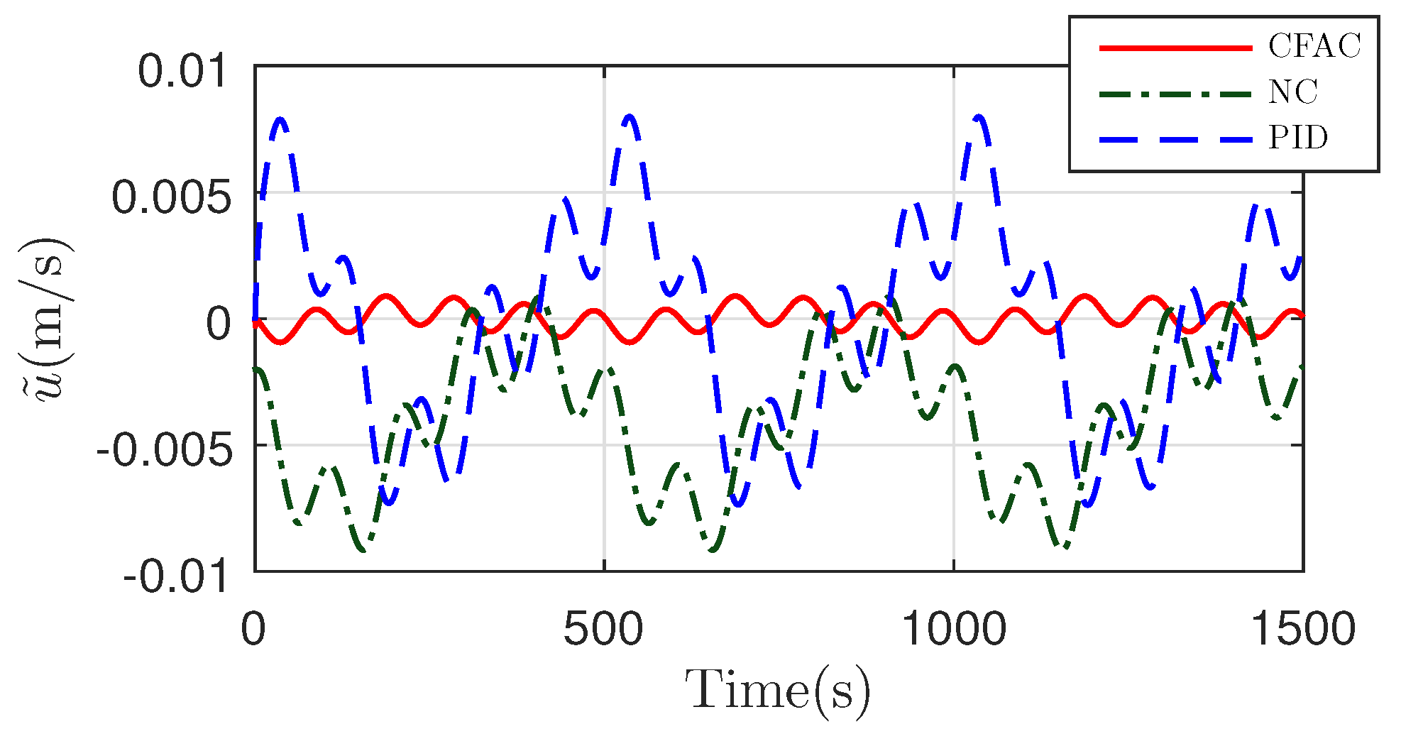
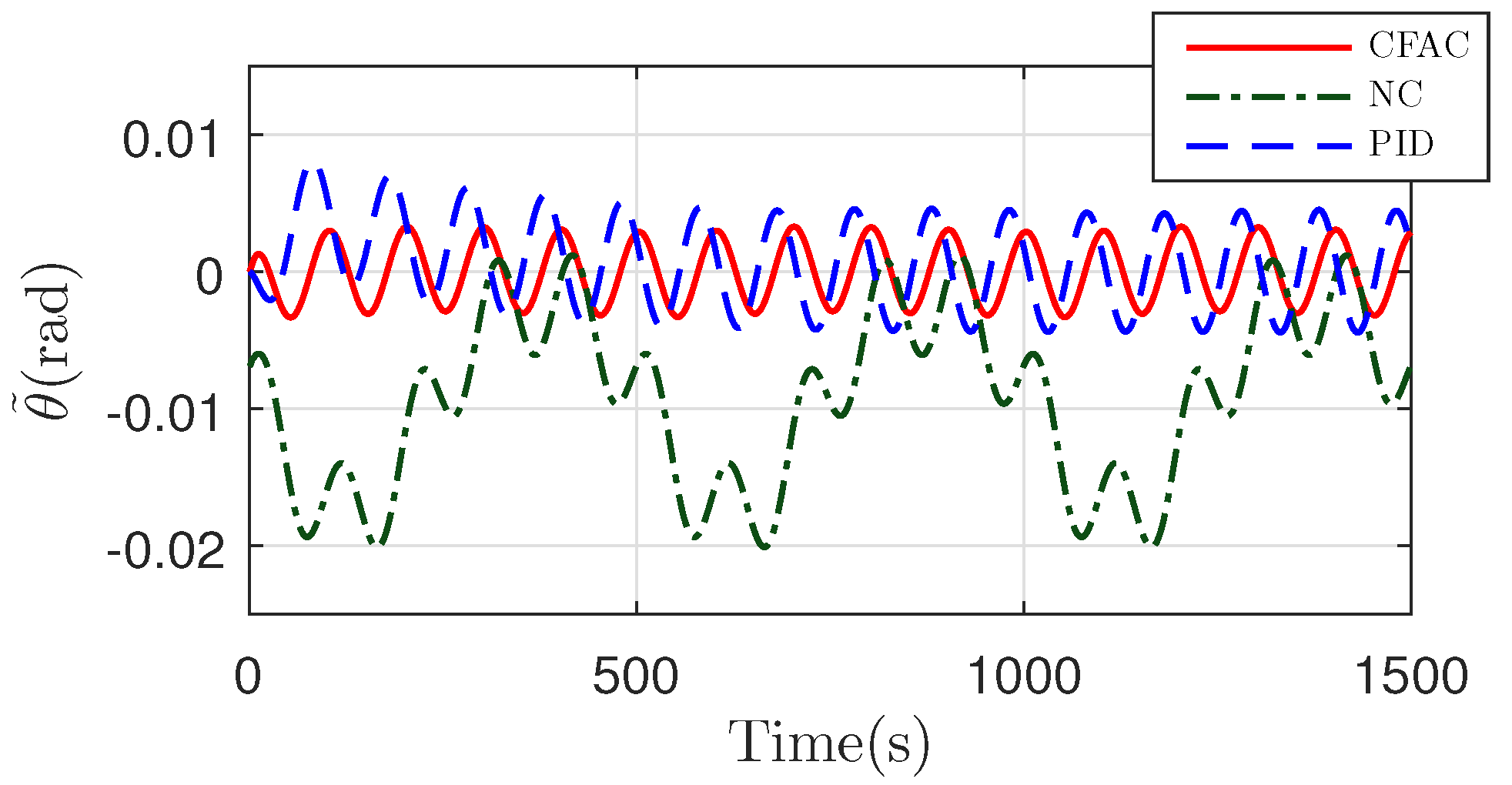
Firstly, the desired velocity is variable, while the desired pitch angle is constant. The tracking performance of velocity is shown in Figure 4 and Figure 5. PID exhibits the largest velocity tracking errors, and NC is a little better than PID. Comparing with NC and PID, CFAC performs much better. Figure 6 and Figure 7 show the pitch angle tracking performance. NC demonstrates the largest tracking errors among three controllers. CFAC is better than PID. The control inputs $U_1$ and $U_2$ are shown in Figure 8 and Figure 9 respectively.

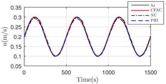
Figure 4. Velocity tracking performance in submerging motion with a variable velocity and constant pitch angle command.

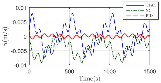
Figure 5. Velocity tracking error in submerging motion with a variable velocity and constant pitch angle command.

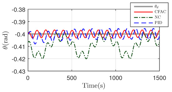
Figure 6. Pitch angle tracking performance in submerging motion with a variable velocity and constant pitch angle command.

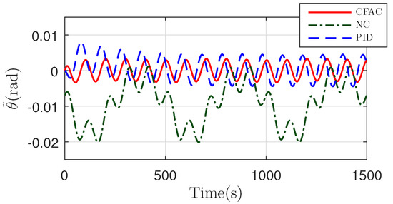
Figure 7. Pitch angle tracking error in submerging motion with a variable velocity and constant pitch angle command.

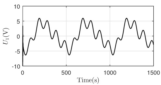
Figure 8. Control input $U_1$ in submerging motion with a variable velocity and constant pitch angle command.

Figure 9. Control input $U_2$ in submerging motion with a variable velocity and constant pitch angle command.

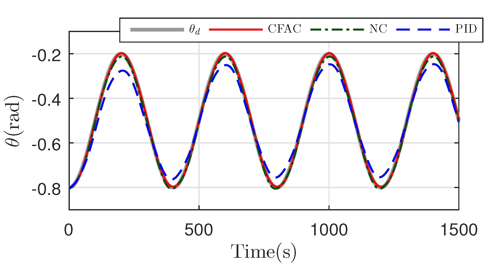
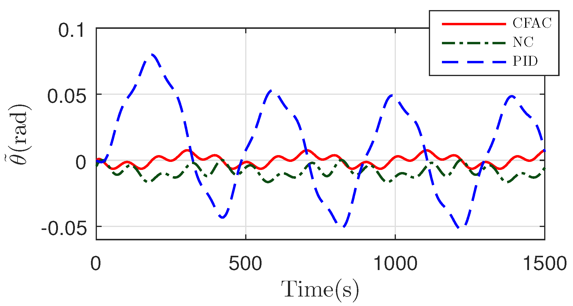
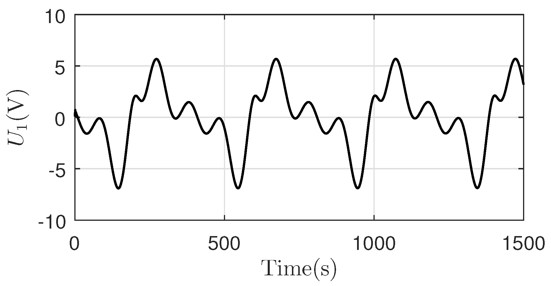
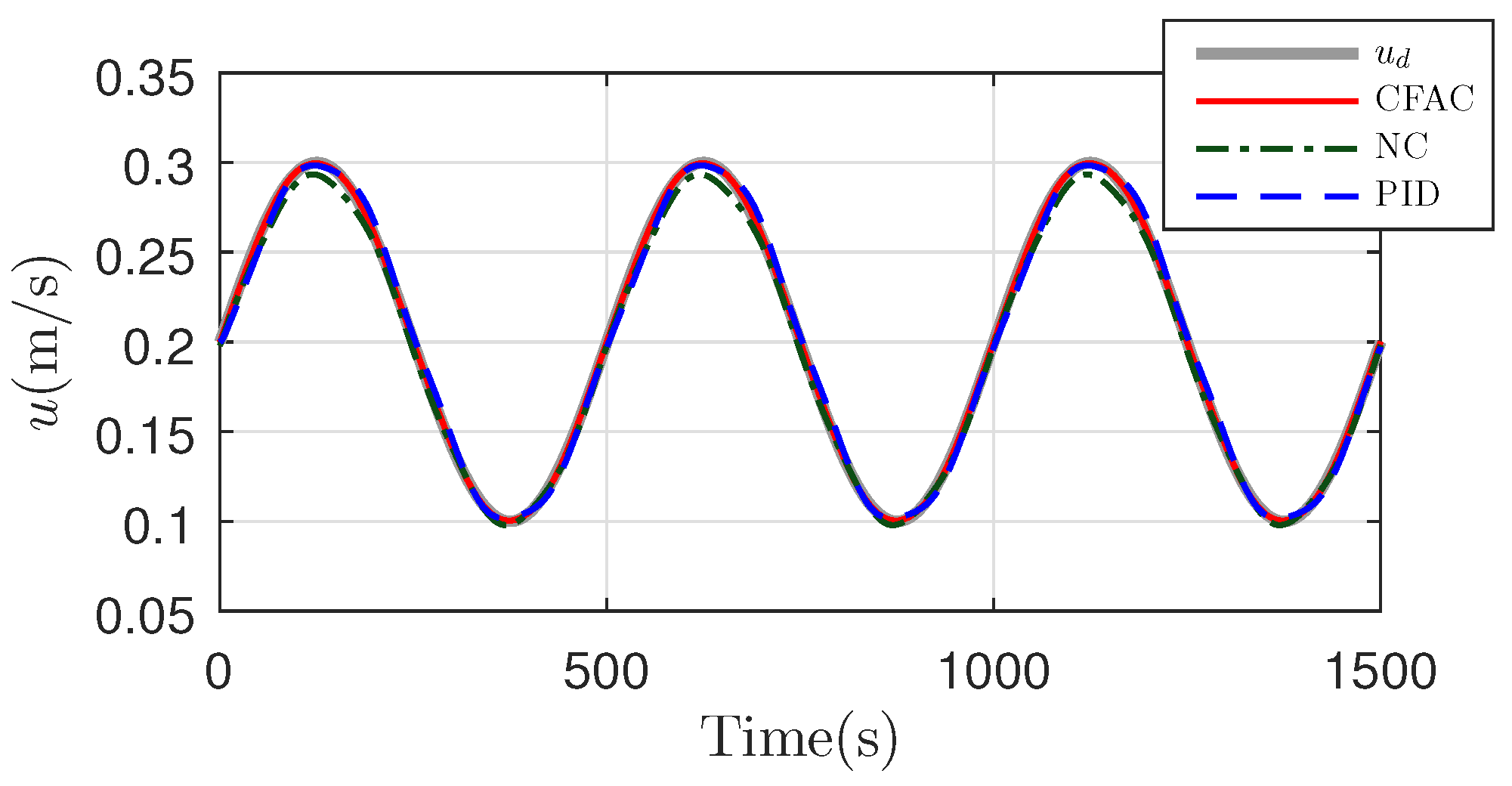
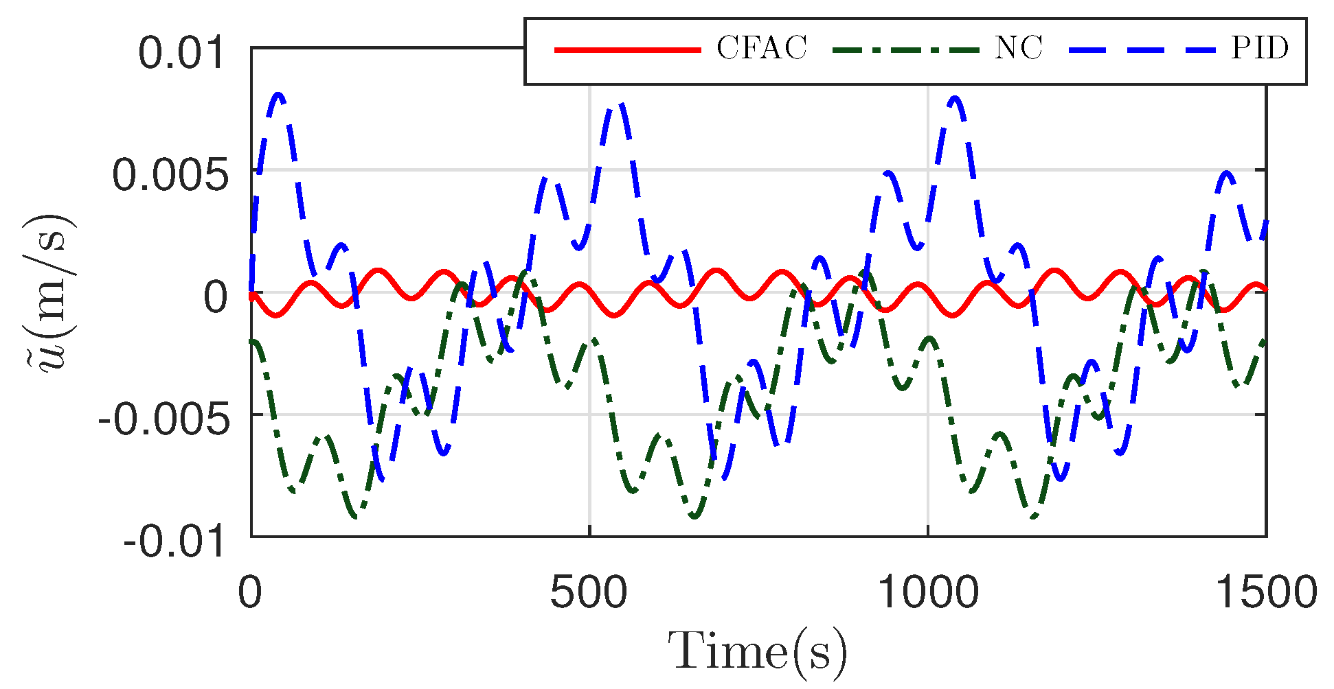
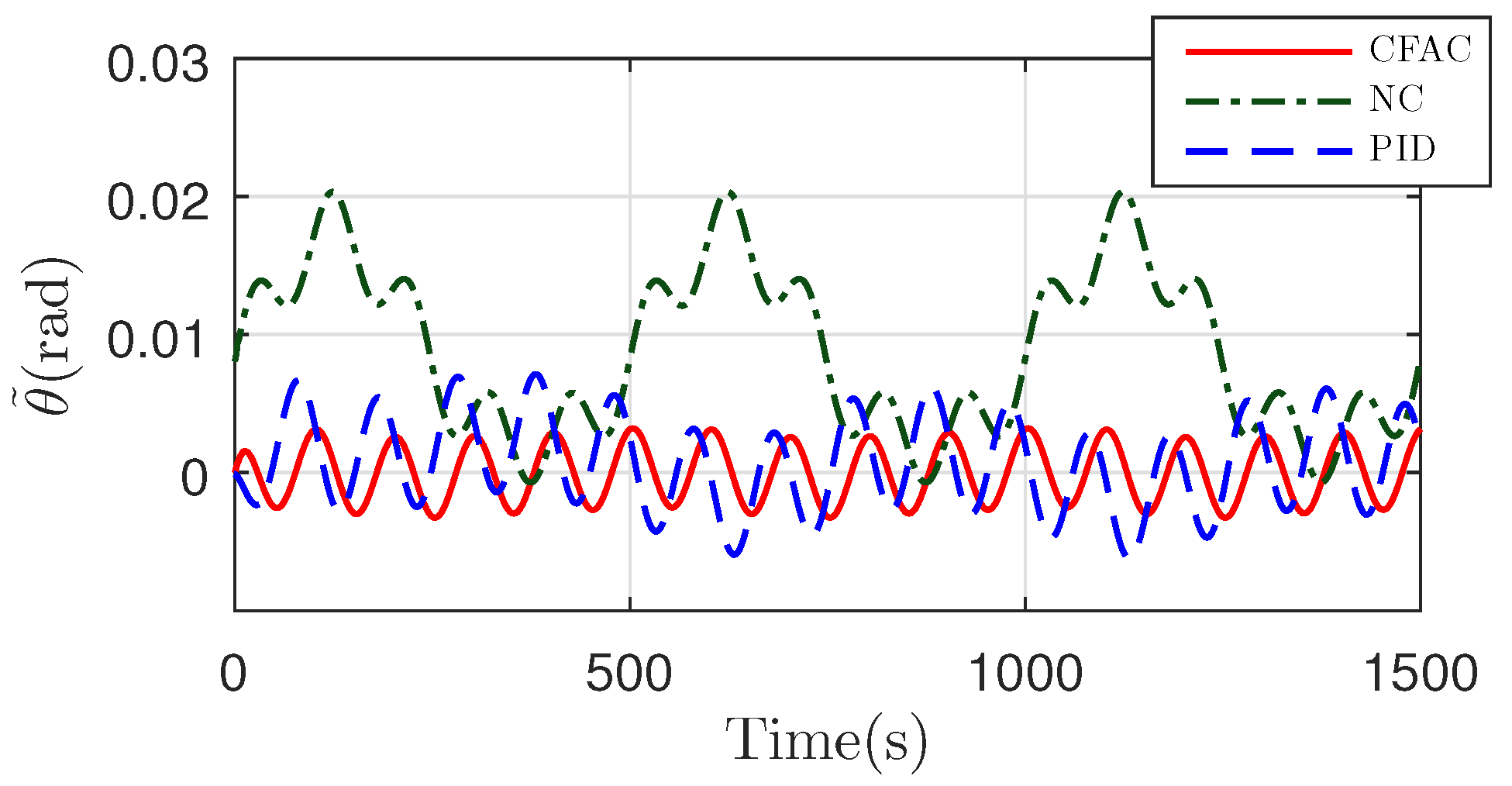
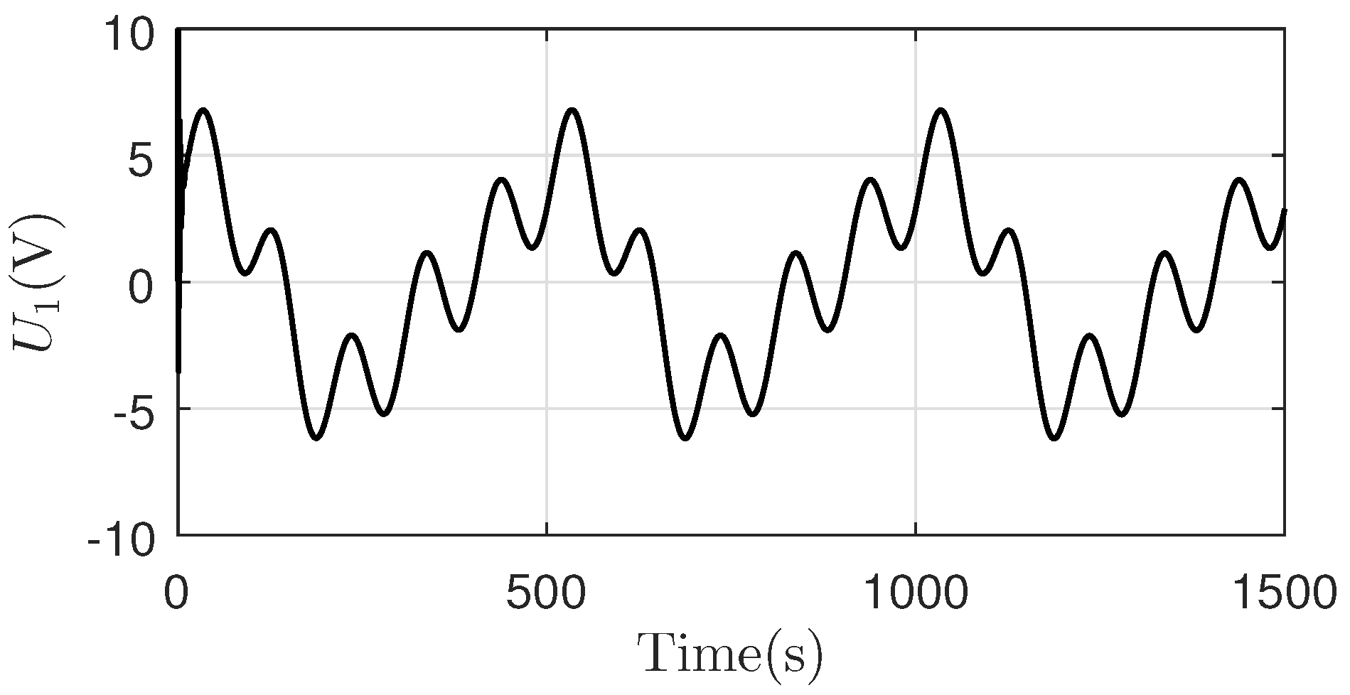
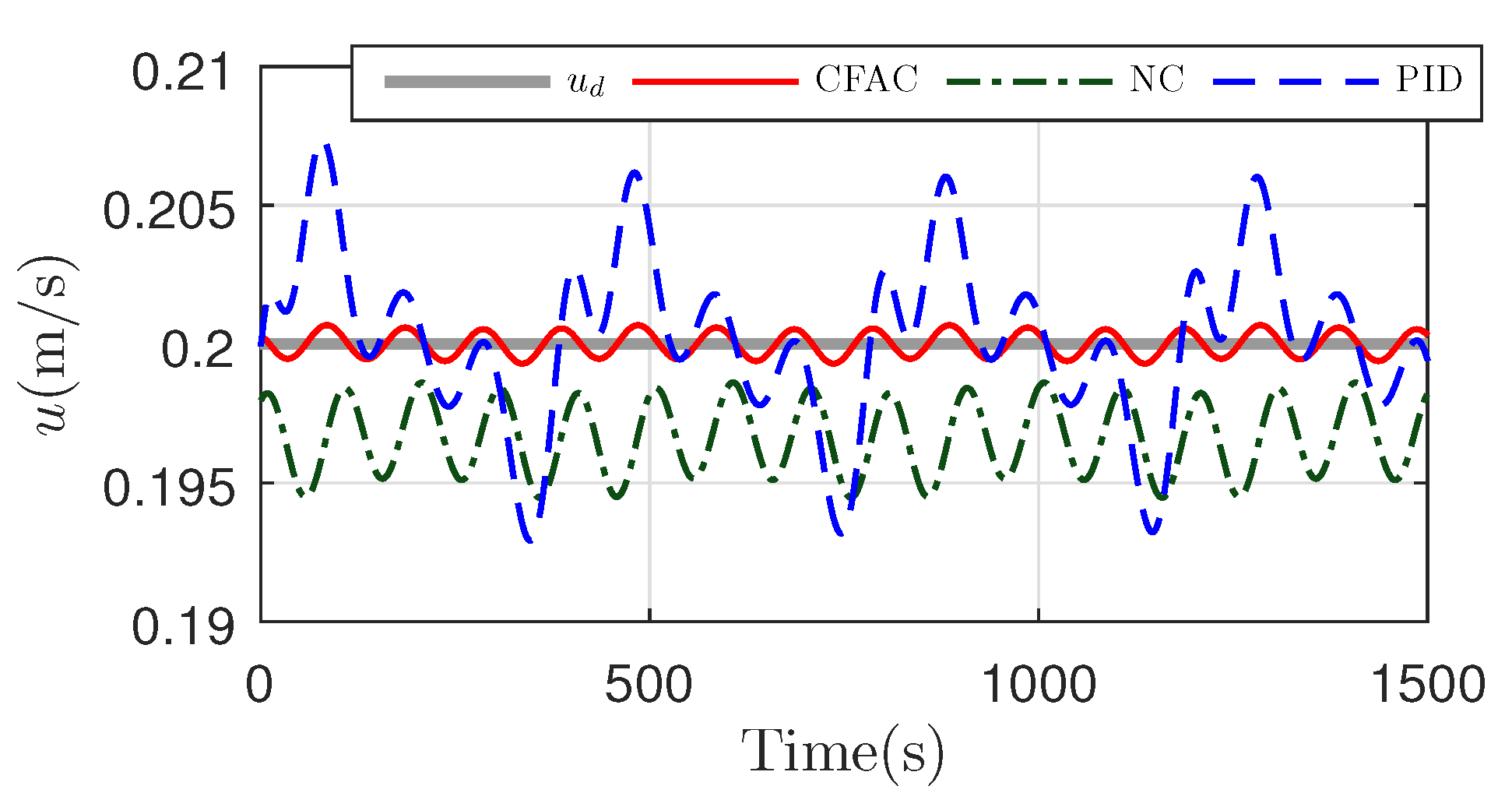
Then, the desired velocity is constant, while the desired pitch angle is variable. Based on Figure 10, Figure 11, Figure 12 and Figure 13, CFAC displays the best tracking performance both in velocity and pitch angle. The control inputs $U_1$ and $U_2$ are shown in Figure 14 and Figure 15 respectively.

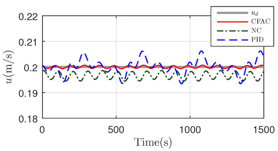
Figure 10. Velocity tracking performance in submerging motion with a constant velocity and variable pitch angle command.

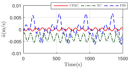
Figure 11. Velocity tracking error in submerging motion with a constant velocity and variable pitch angle command.

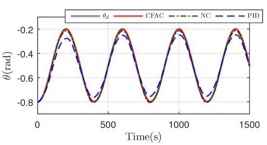
Figure 12. Pitch angle tracking performance in submerging motion with a constant velocity and variable pitch angle command.

Figure 13. Pitch angle tracking error in submerging motion with a constant velocity and variable pitch angle command.

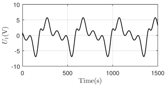
Figure 14. Control input $U_1$ in submerging motion with a constant velocity and variable pitch angle command.

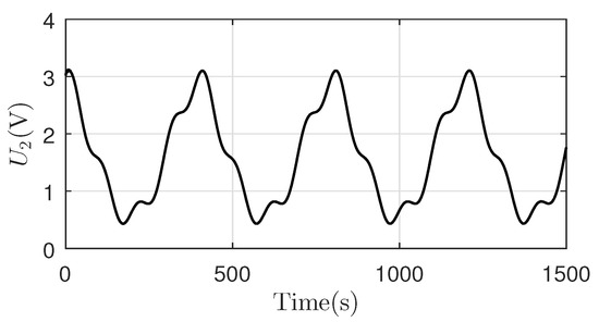
Figure 15. Control input $U_2$ in submerging motion with a constant velocity and variable pitch angle command.

It could be seen that nonlinear controller without parameter adaption may not achieve a better result than the traditional PID controller. NC works based on accurate model compensation. If parameters and disturbances in the model cannot be obtained precisely, NC may not demonstrate a good performance. In the meanwhile, PID does not depend on accurate model, and can obtain good results in a specific working condition. The drawback of PID is that the control parameters in PID only guarantee some specific working conditions. CFAC takes the advantages of adaptive control, which could attenuate the influence of parameter variation and external disturbance.

4.2. Case 2: Motion Control during Floating in Vertical Plane

To validate the robustness of CFAC, the simulation of floating motion from seabed to sea surface in vertical plane is also conducted. Same parameter initial values and disturbances as Case 1 are applied. Firstly, the desired velocity is variable, while the desired pitch angle is constant. The velocity tracking performance is shown in Figure 16 and Figure 17. The pitch angle tracking performance is shown in Figure 18 and Figure 19. The control inputs $U_1$ and $U_2$ are shown in Figure 20 and Figure 21 respectively.

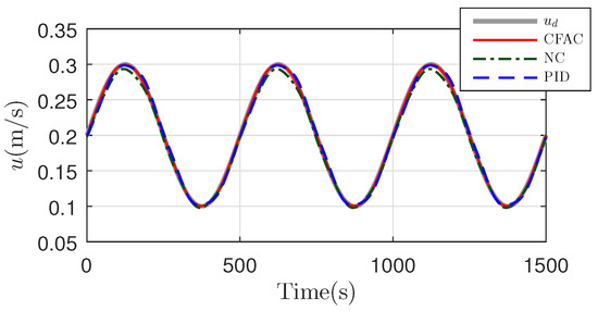
Figure 16. Velocity tracking performance in floating motion with a variable velocity and constant pitch angle command.

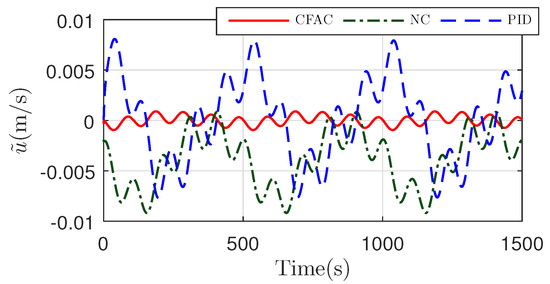
Figure 17. Velocity tracking error in floating motion with a variable velocity and constant pitch angle command.

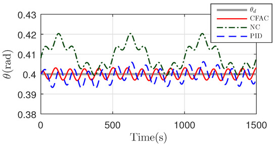
Figure 18. Pitch angle tracking performance in floating motion with a variable velocity and constant pitch angle command.

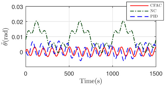
Figure 19. Pitch angle tracking error in floating motion with a variable velocity and constant pitch angle command.

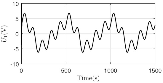
Figure 20. Control input $U_1$ in floating motion with a variable velocity and constant pitch angle command.

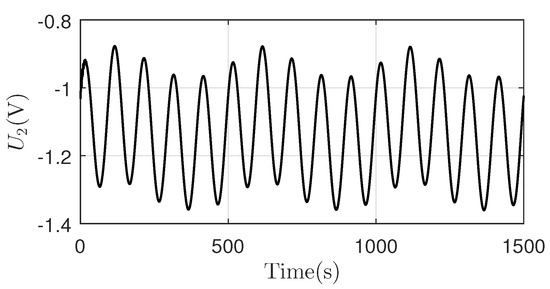
Figure 21. Control input $U_2$ in floating motion with a variable velocity and constant pitch angle command.

Secondly, the desired velocity is constant, and the desired pitch angle is variable. Figure 22, Figure 23, Figure 24 and Figure 25 show the tracking performance. Similar as Case 1, CAFC achieves the best tracking performance, comparing with NC and PID. PID demonstrates the worst pitch angle tracking performance in Figure 24 and Figure 25. Because the disturbance in the pitch angle loop and influence of hydraulic buoyancy regulating system hinder PID achieve good pitch angle tracking performance. The control inputs $U_1$ and $U_2$ are shown in Figure 26 and Figure 27 respectively.

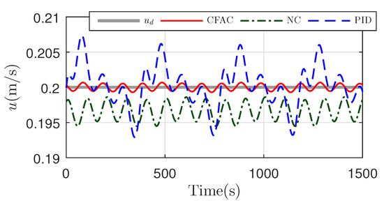
Figure 22. Velocity tracking performance in floating motion with a constant velocity and variable pitch angle command.

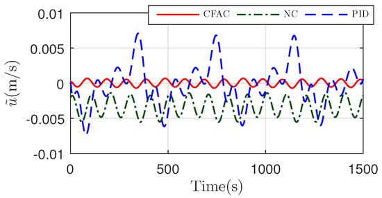
Figure 23. Velocity tracking error in floating motion with a constant velocity and variable pitch angle command.

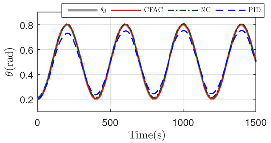
Figure 24. Pitch angle tracking performance in floating motion with a constant velocity and variable pitch angle command.

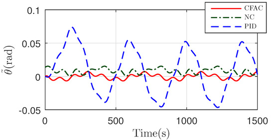
Figure 25. Pitch angle tracking error in floating motion with a constant velocity and variable pitch angle command.

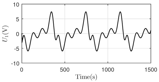
Figure 26. Control input $U_1$ in floating motion with a constant velocity and variable pitch angle command.

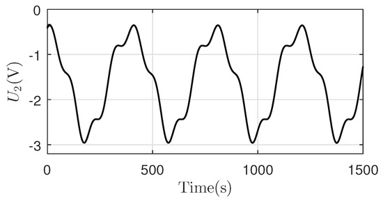
Figure 27. Control input $U_2$ in floating motion with a constant velocity and variable pitch angle command.

According to Case 1 and Case 2, CFAC shows its excellent motion control ability in both submerging and floating process in vertical plane. The switch process between submerging and floating process is not considered, because the switch process could be treated as an open-loop control process with depth as the command. After the switch process, closed-loop motion control can be executed again, which guarantees the completion of oceanic observation tasks.

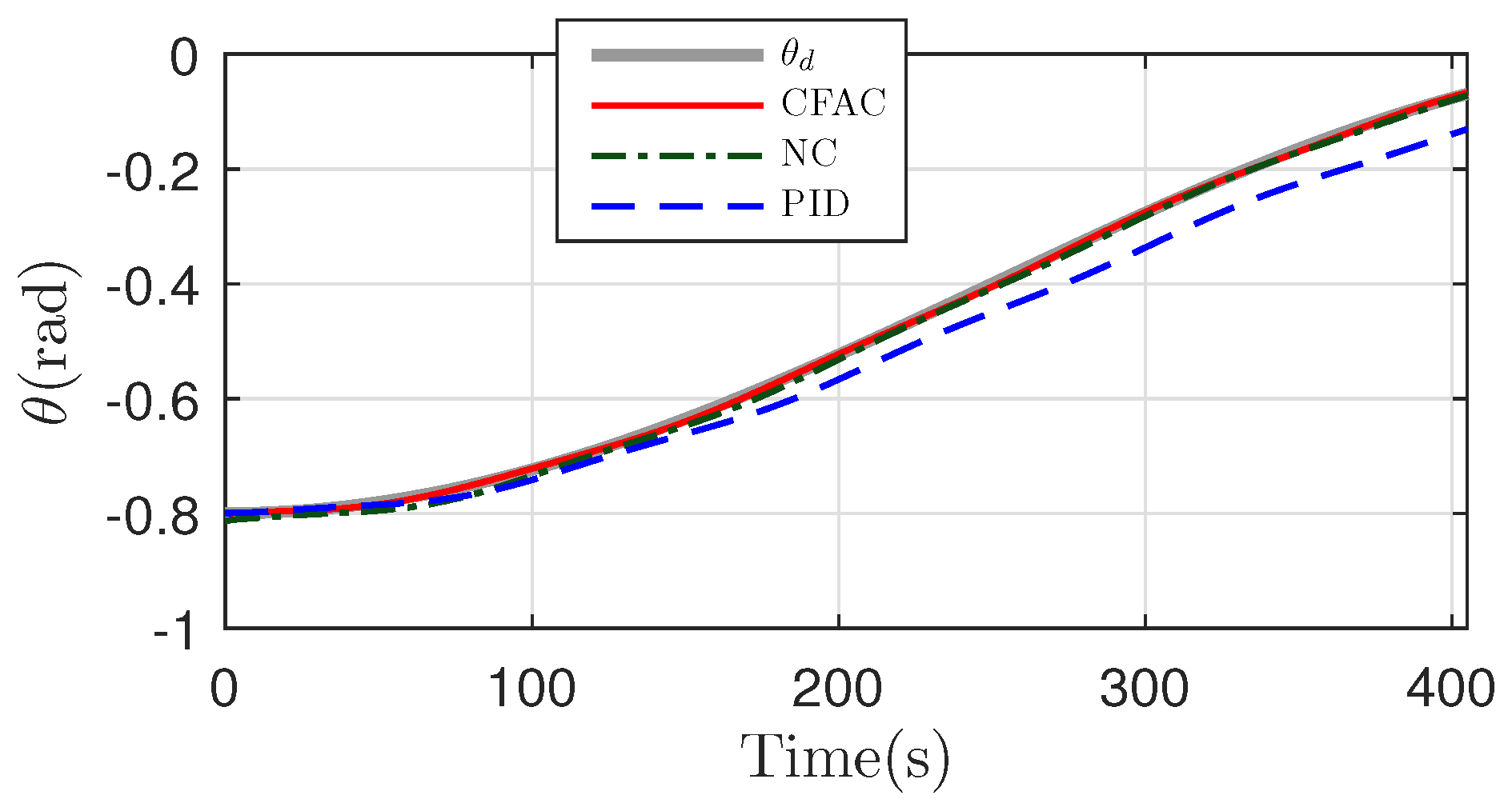
4.3. Case 3: Motion Control in Virtual Mooring

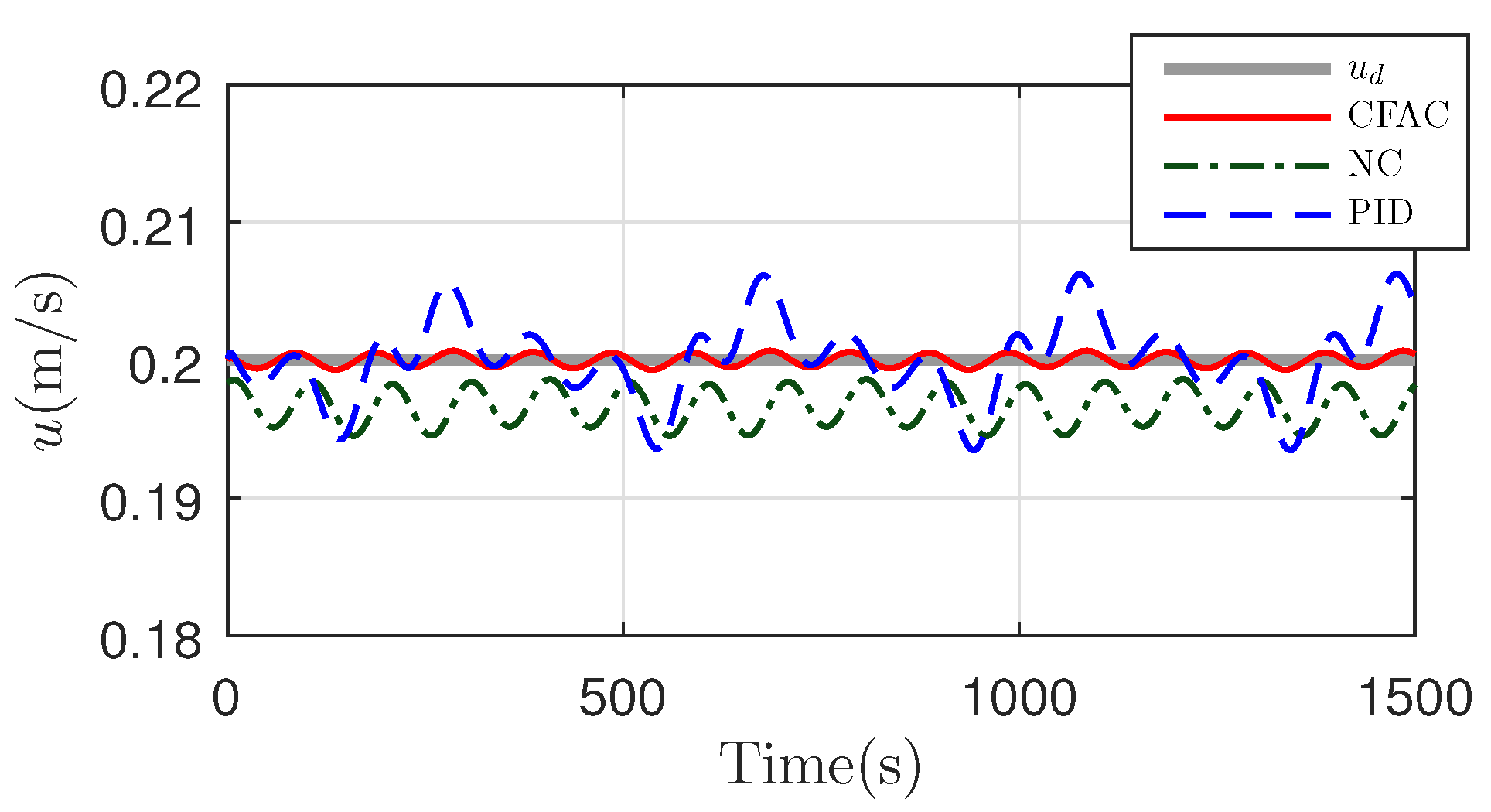
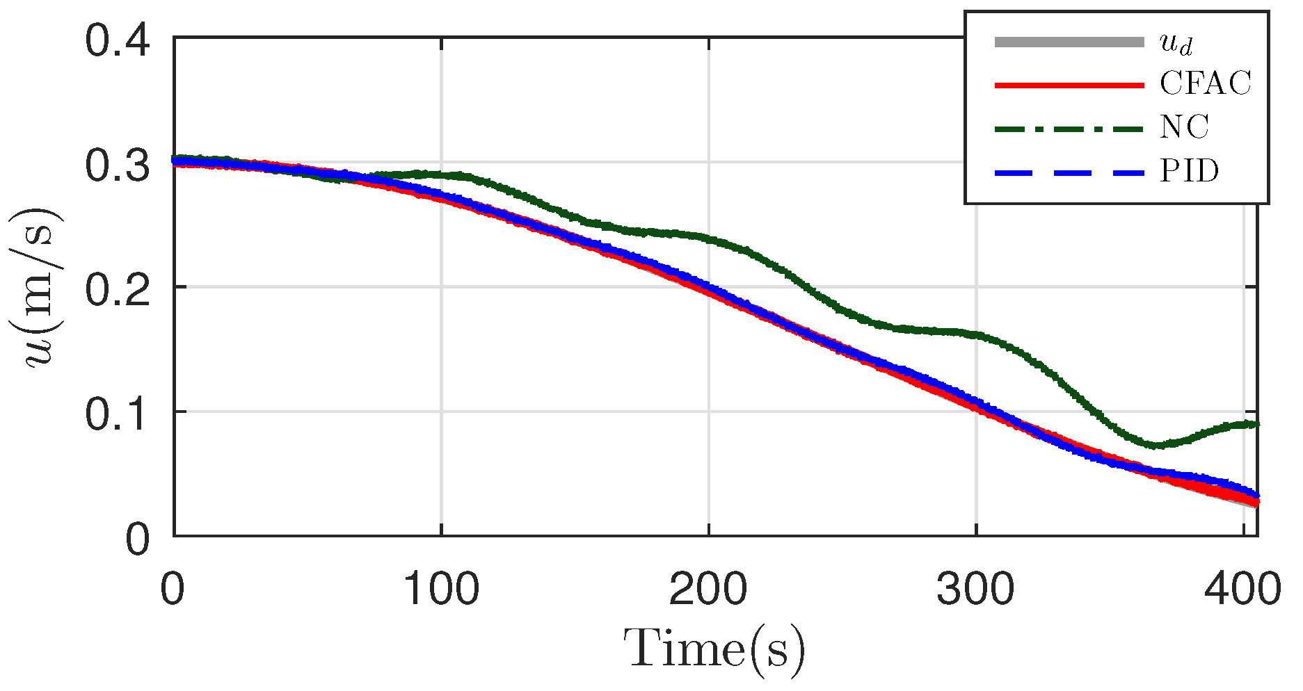
To explore the performance of CFAC further, simulation of virtual mooring in the submerging process is conducted. Same parameter initial values and disturbances as Case 1 are applied. The desired trajectories of velocity and pitch angle are described in Figure 28 and Figure 29. When the pitch angle $\theta$ approaches zero, $\Delta B_e^0$ in (16) will become infinite. In addition, the condition $u>>w$ (u is much larger than w) will be no more satisfied, if velocity u tends to zero. Therefore, the terminal of the desired trajectory is set as $u_d=0.03$ m/s and ${\theta }_d=-0.08$ rad, since low speed and small pitch angle will reduce the impact during virtual mooring. Once the desired trajectory reaches the terminal, the underwater glider will shift to open-loop buoyancy regulating and realize the final mooring. Because noises always exist in the practical measurement, especially velocities, white noises are imposed on the feedback of u, w and q in the simulation.

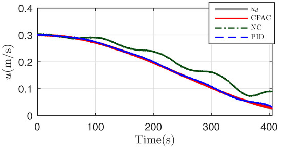
Figure 28. Velocity tracking performance in virtual mooring.

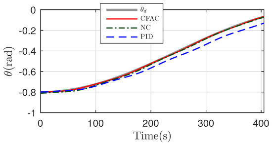
Figure 29. Pitch angle tracking performance in virtual mooring.

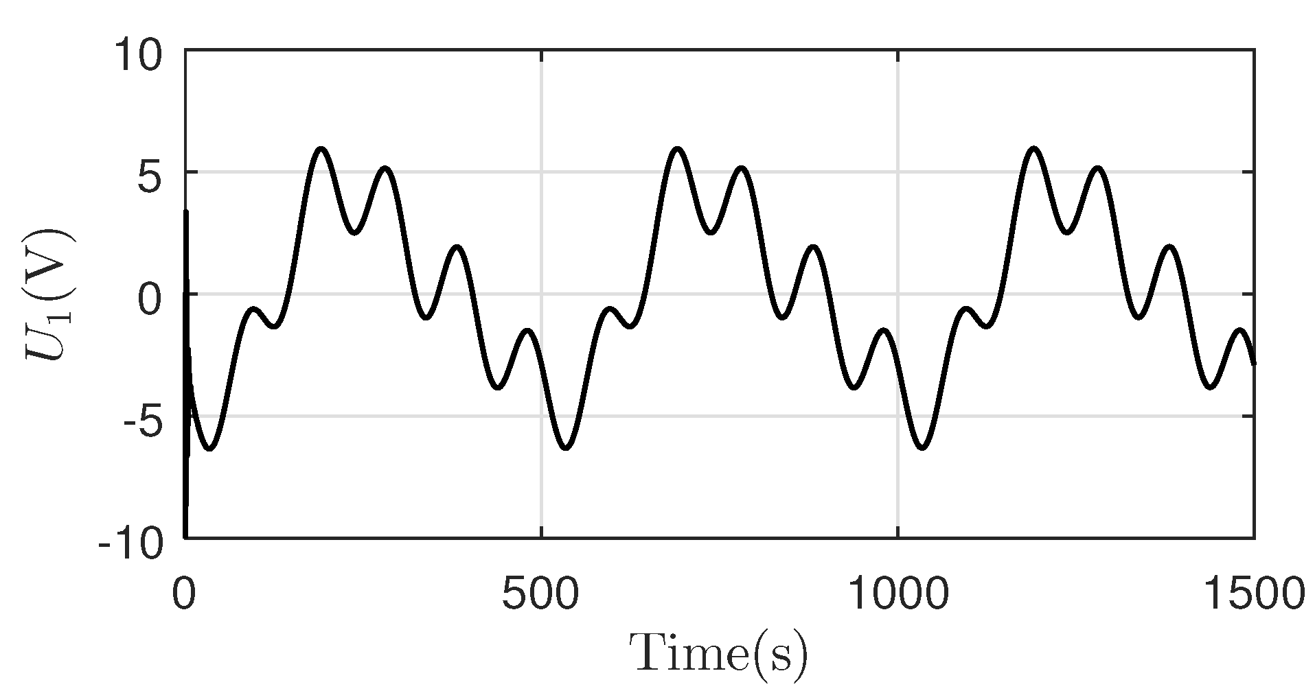
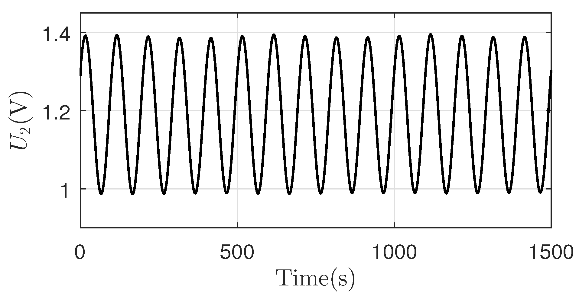
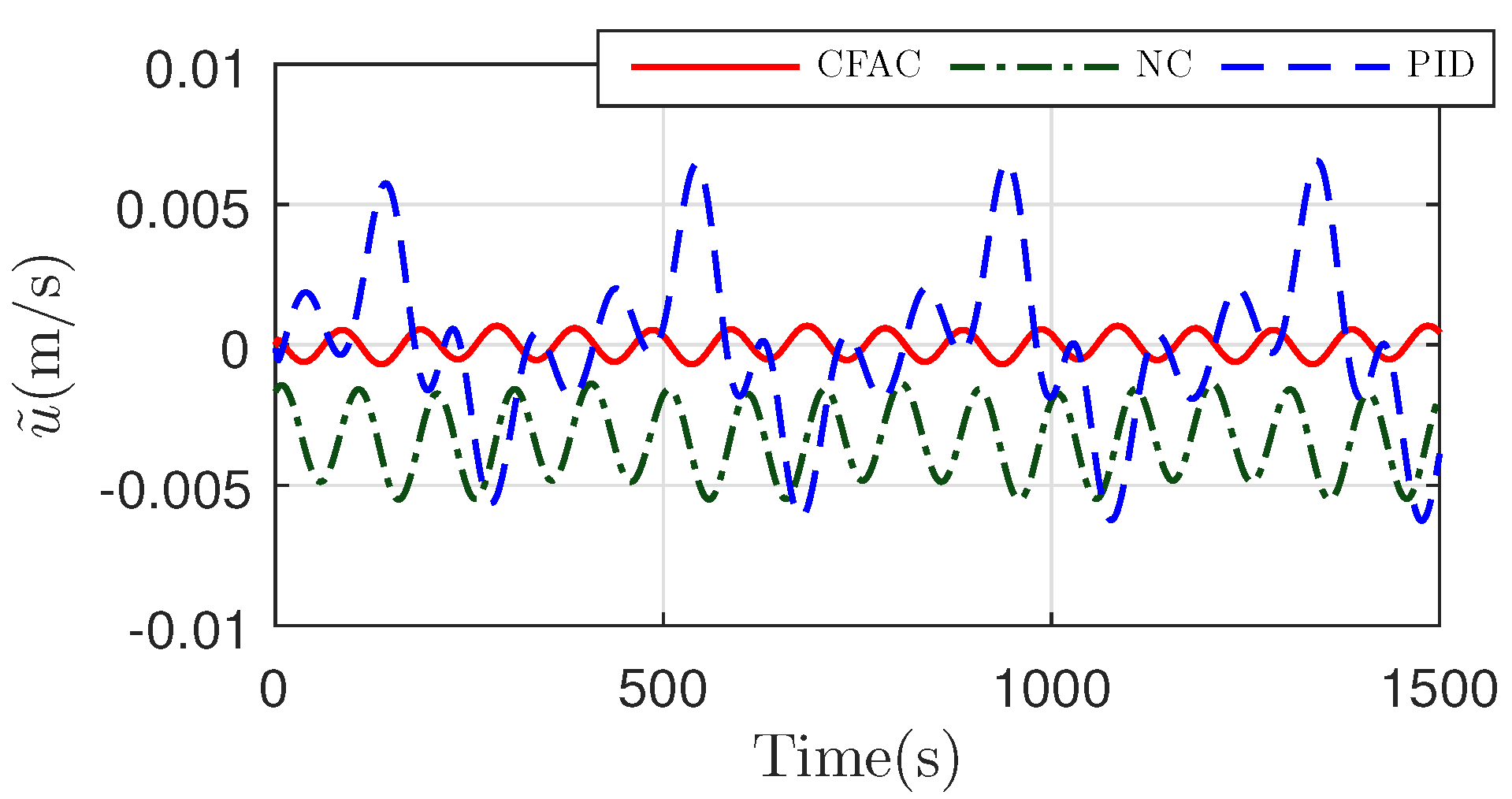
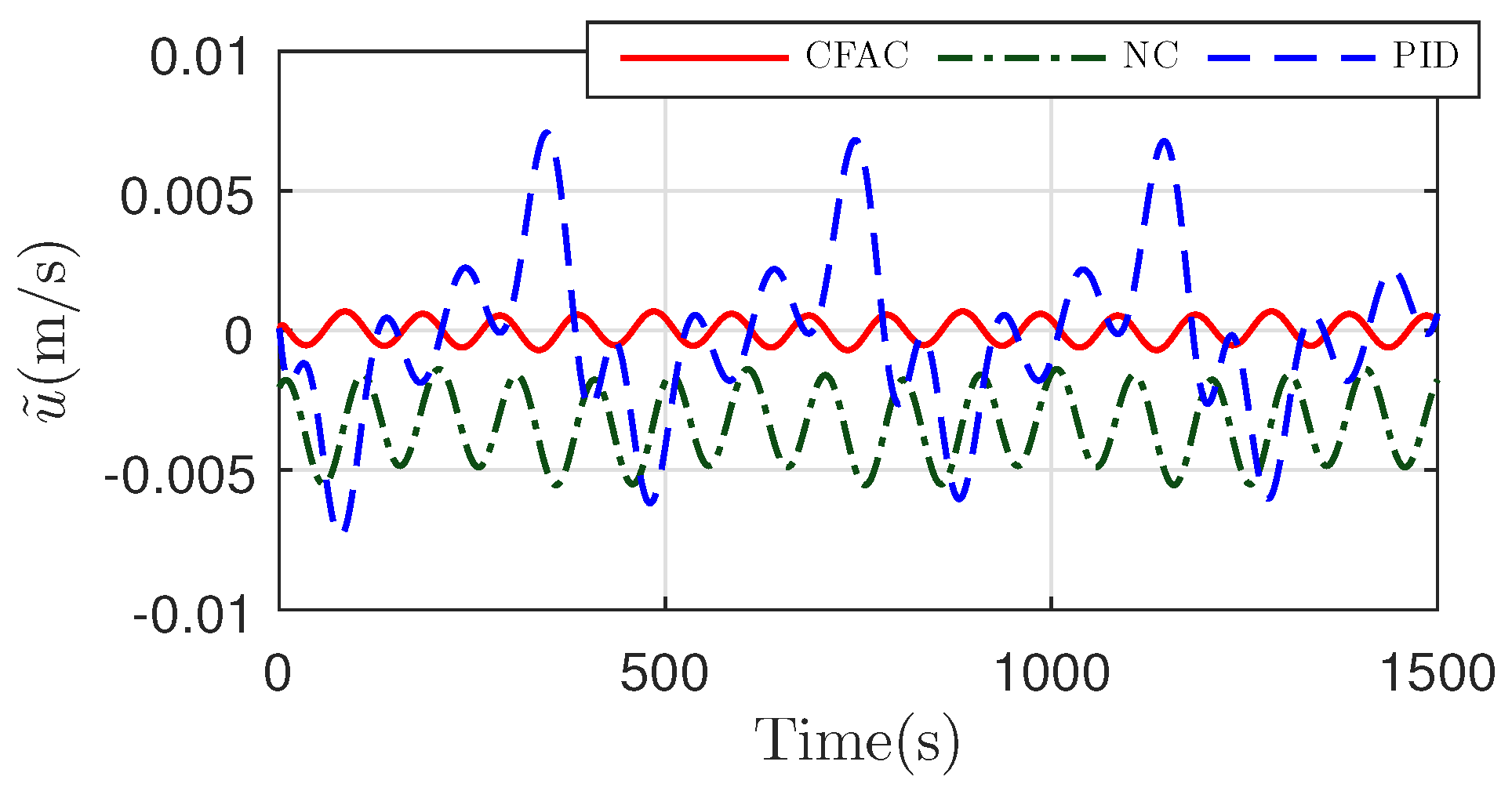
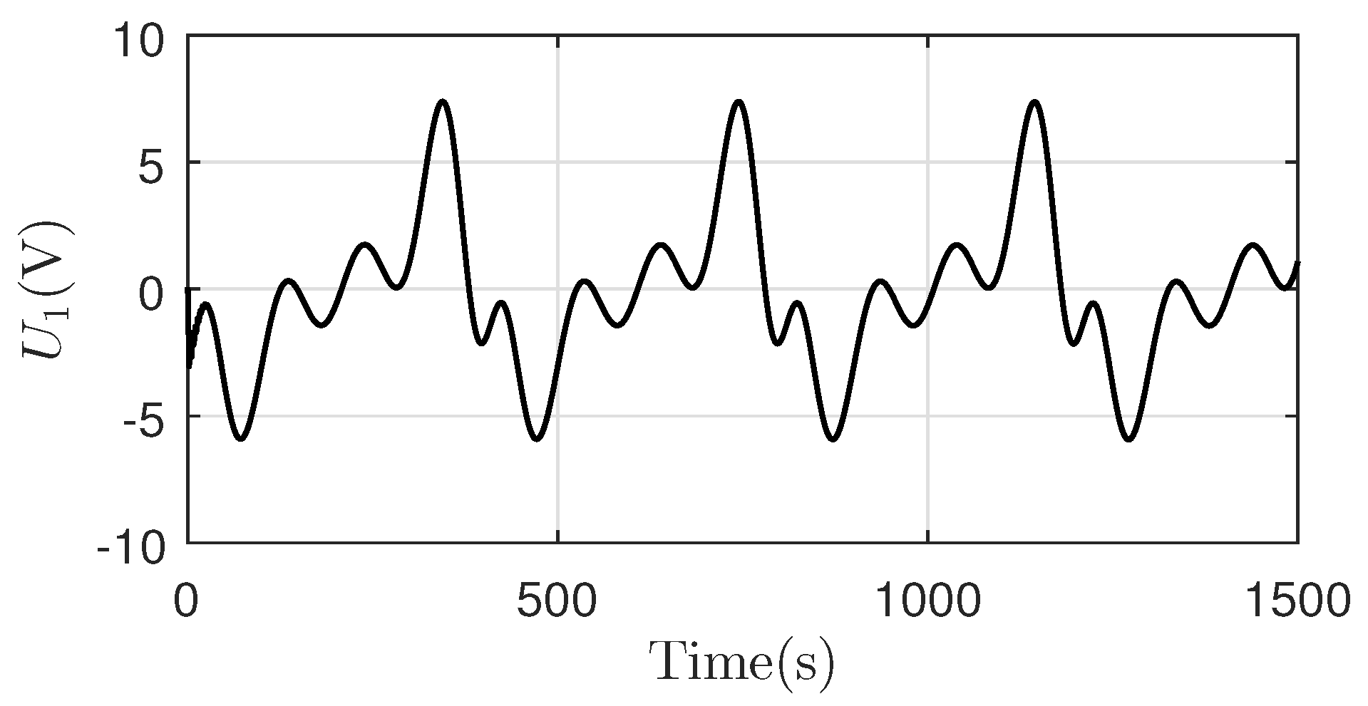
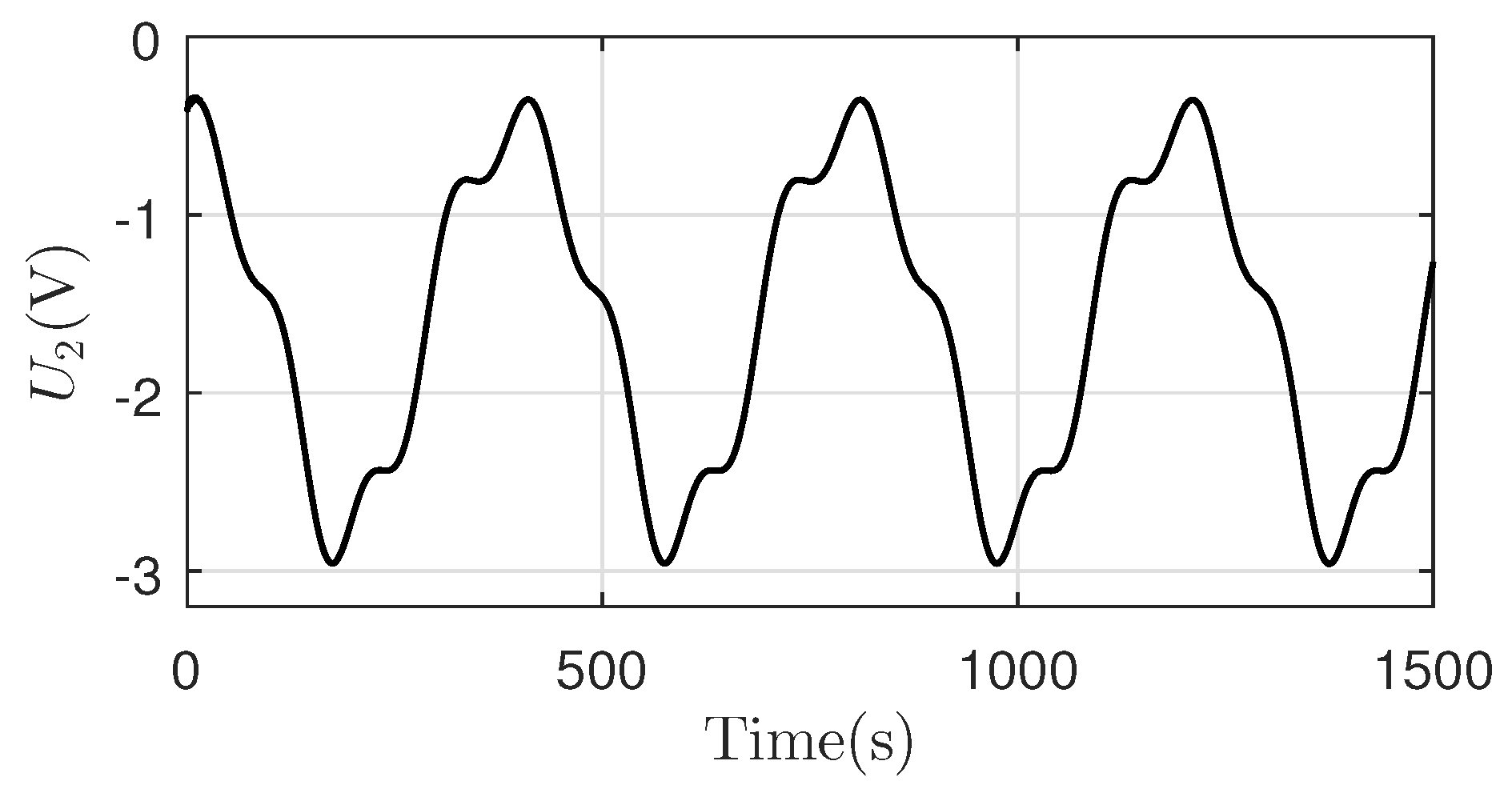
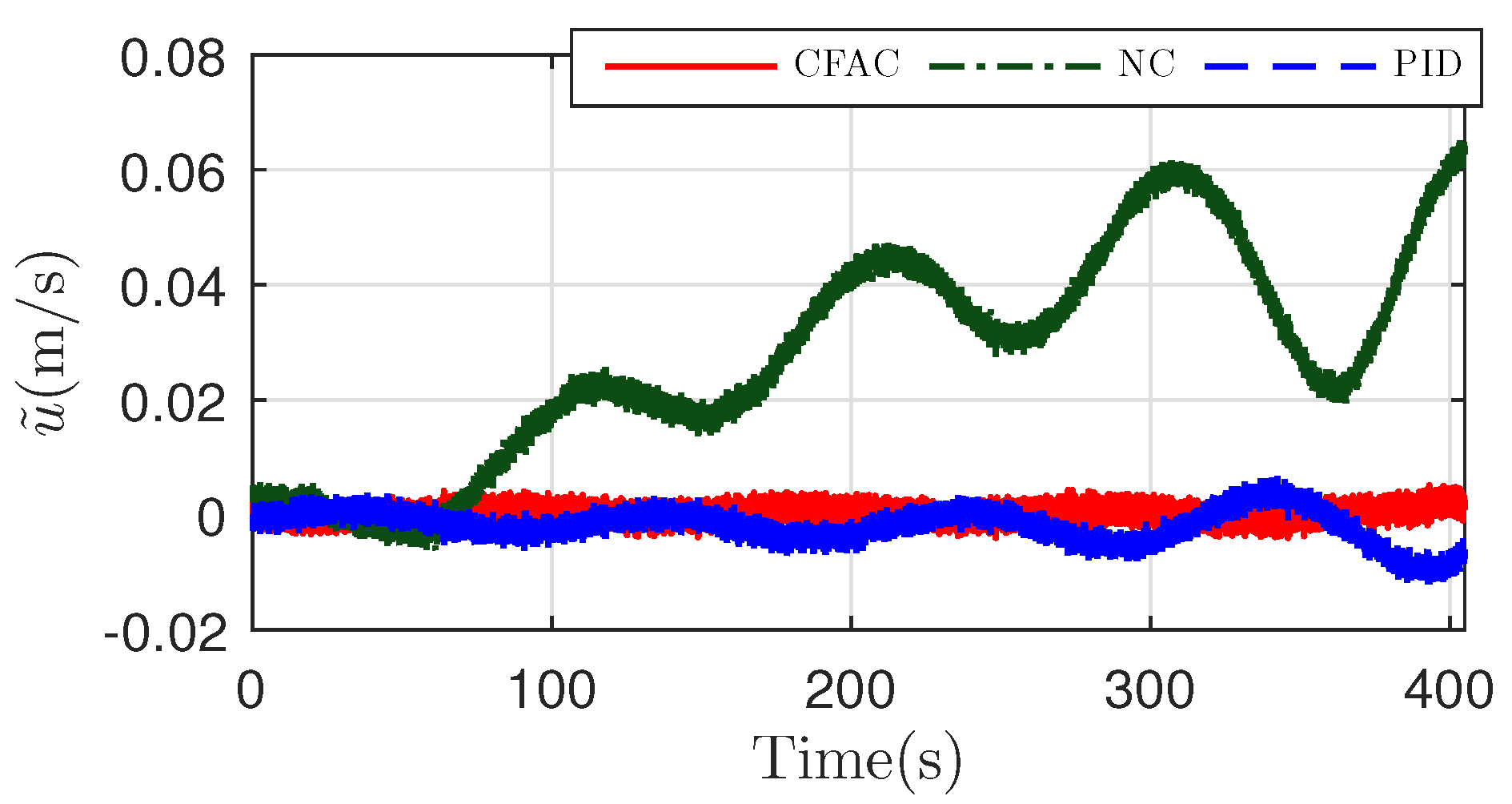
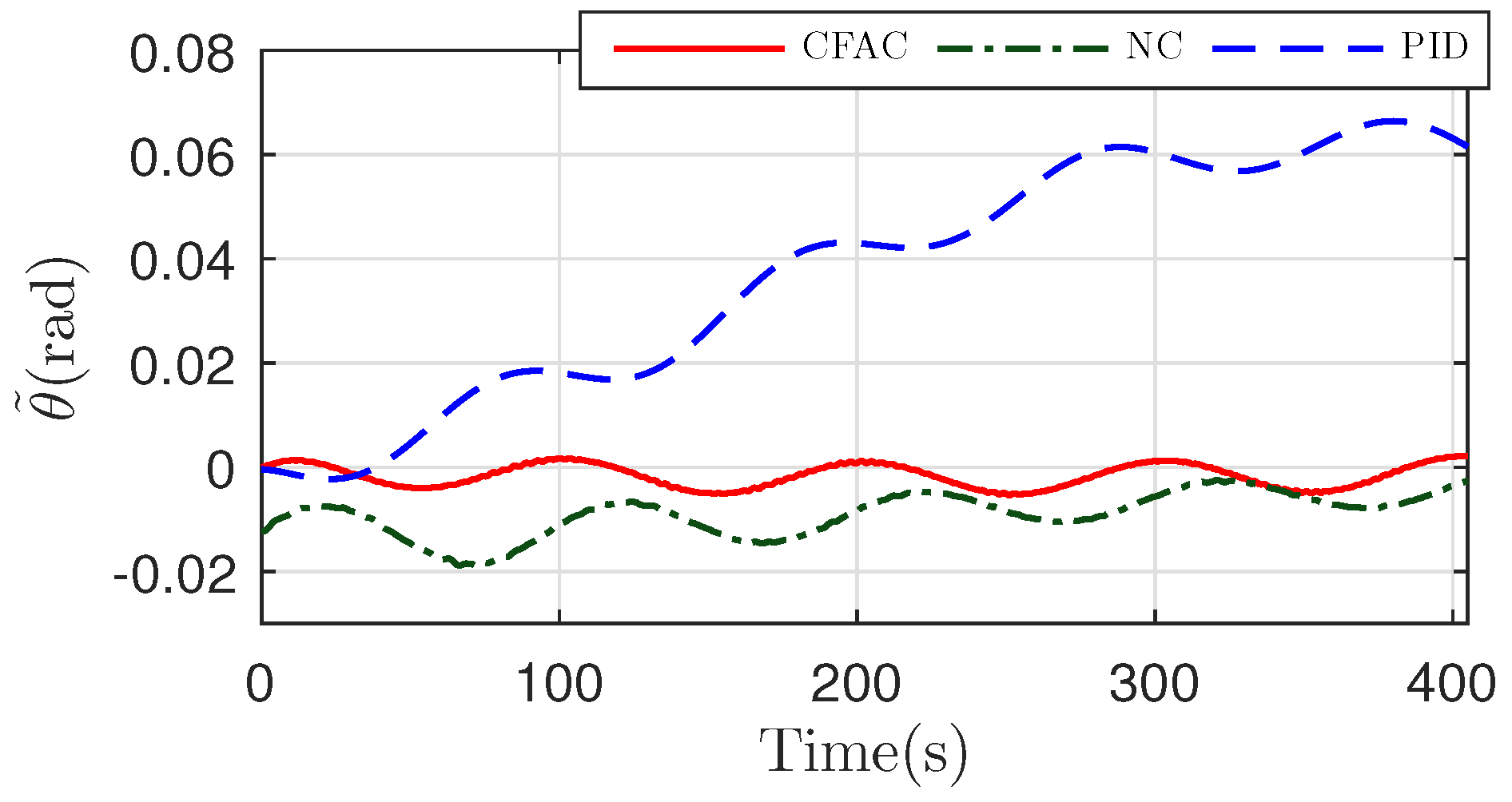
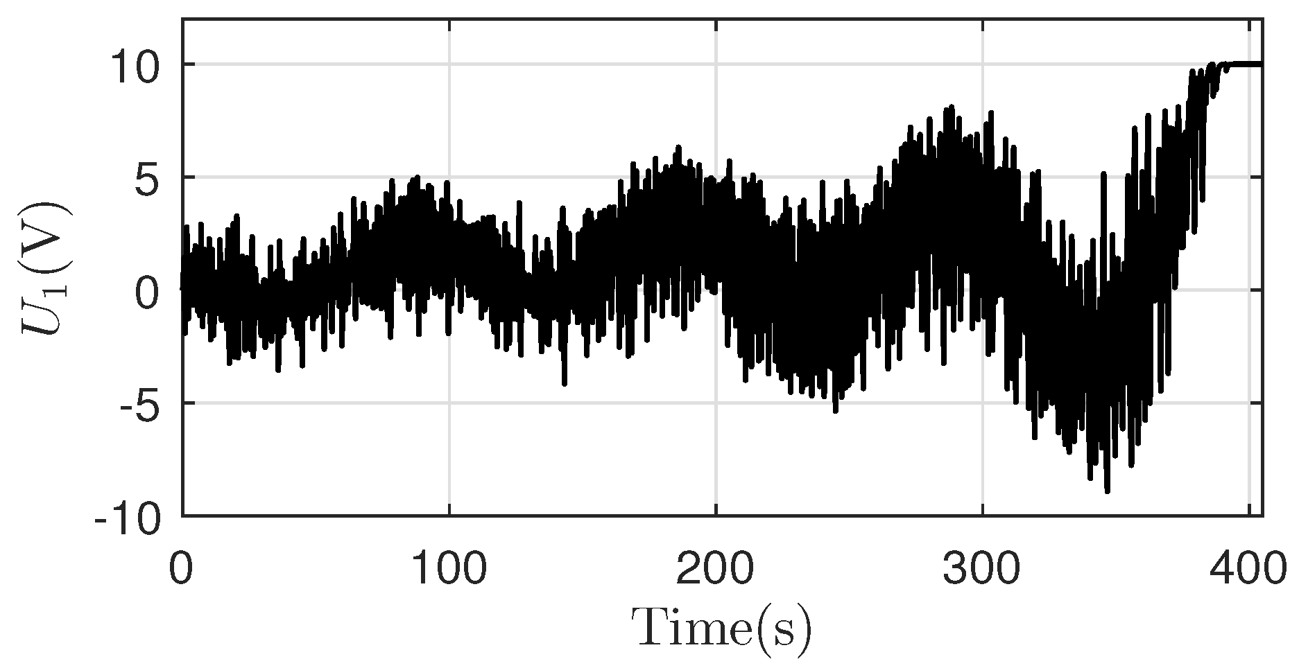
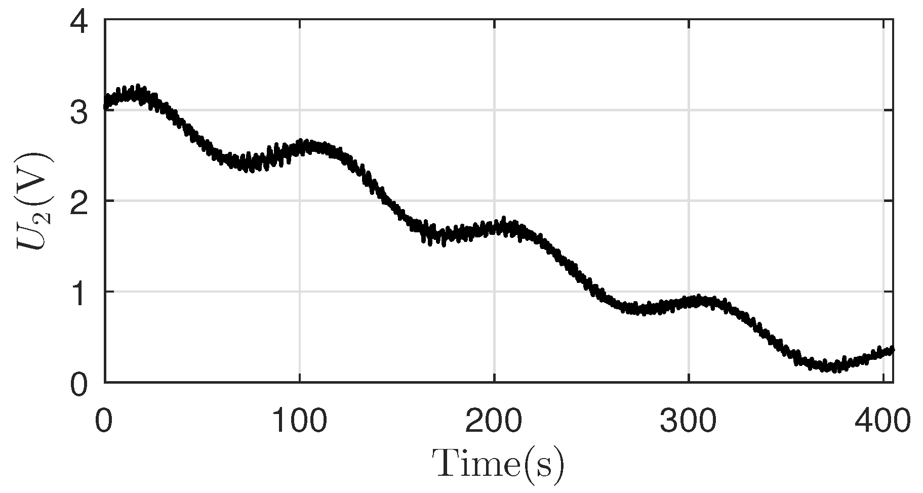
Figure 28 and Figure 30 show the velocity tracking performance. The velocity tracking errors of NC is larger than PID and CFAC. It can be seen that both the absolute value and amplitude of tracking error are much larger in NC. The reason is not only the parameter uncertainties and disturbances, but also the imposed measurement noises. However, in the meantime, PID also achieves a good performance as CFAC. PID strategy is only based on the feedback. The low dynamics of the hydraulic buoyancy regulating system and velocity response can reduce the noises imposed on the feedback of u, w and q. In addition, the parameter adaption of CFAC could not reach its best in a short working time. In CFAC, adaptive strategy compensates the parameter uncertainties and disturbances, while command filter attenuates the calculation explosion of derivatives caused by measurement noises in the backstepping process. The pitch angle tracking performance is shown in Figure 29 and Figure 31. CFAC still holds the best tracking performance. The control inputs $U_1$ varies acutely due to the imposed noises on feedback velocities as shown in Figure 32. $U_1$ finally reaches its saturation $10V$, that indicates a small velocity and pitch angle command is beyond the ability of the underwater glider. Control input $U_2$ is shown in Figure 33. $U_2$ does not vary dramatically like $U_1$, because the dynamics of pitch angle is lower than the one of velocity.

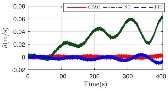
Figure 30. Velocity tracking error in virtual mooring.

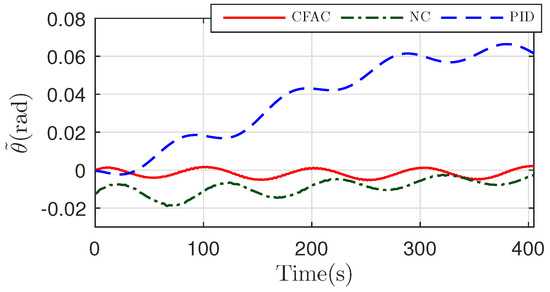
Figure 31. Pitch angle tracking error in virtual mooring.

Figure 32. Control input $U_1$ in virtual mooring.

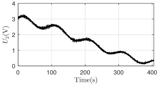
Figure 33. Control input $U_2$ in virtual mooring.

In CFAC, command filter deals with the command saturation and calculation of derivatives in the underwater glider control system. Equation (45) guarantees that $\overline{u}$, $\Delta {\overline{B}}_e$, $\overline{s}$ and ${\overline{r}}_p$ will become zero asymptotically, which are different from the expected tracking errors $\tilde{u}$, $\Delta {\tilde{B}}_e$, $\tilde{s}$ and ${\tilde{r}}_p$. Since the dynamics of u and $\theta$ of the underwater glider is not high based on (13), command filter can be applied to make CFAC work with a suitable response time to avoid overshoot. Taking $\tilde{u}$ for example, $\tilde{u}=\overline{u}+{\chi }_1$ based on (17), and ${\dot{\chi }}_1=-c_1{\chi }_1+\frac{sin\theta }{M_{f_1}}\left(\Delta B_e^{*}-\Delta B_e^0\right)$, ${\chi }_1$ is the first-order filter output of $\frac{sin\theta }{M_{f_1}}\left(\Delta B_e^{*}-\Delta B_e^0\right)$. $\Delta B_e^{*}$ is the filter output of $\Delta B_e^0$ through command filter in Figure 2. The error between $\Delta B_e^{*}$ and $\Delta B_e^0$ could become small enough to make ${\chi }_1$ converge to zero, that is possible because the dynamics of the underwater glider is not high. As a consequence, $\tilde{u}$ will approach zero, once $\overline{u}$ and ${\chi }_1$ converge to zero. In a same way, $\Delta {\tilde{B}}_e$, $\tilde{s}$ and ${\tilde{r}}_p$ can be proved to approach zero.

In practice use, ${\xi }_i$$(i=1,2,3,4)$ in CFAC is chosen as 1, which is the critical damping ratio of the second-order system and could avoid overshoot and oscillation during command filtering. ${\omega }_{ni}$$(i=1,2,3,4)$ is chosen based on the dynamics of the underwater glider and desired trajectory. A large ${\omega }_{ni}$ may introduce the influence of measurement noises, and cause overshoot and oscillation. A small ${\omega }_{ni}$ cannot eliminate the filter error and lead to the final control error. Hence, a balance of ${\omega }_{ni}$ should be kept. Command saturation keeps the calculated control command in a sound range, which is important for low dynamic systems, such as underwater gliders. Once command saturation works, the underwater glider cannot track the desired trajectory. It means that the dynamics or amplitude of the expected trajectory is beyond the response of controlled system.

5. Conclusions

This paper developed a detailed system mathematical model and a command filtered adaptive control strategy for underwater gliders, whose system dynamics is low and working condition is complicated. It will help improve the maneuverability and motion tracking performance in the oceanic observation tasks. Underwater gliders are driven by a hydraulic buoyancy regulating system and a movable mass. A detailed system dynamic model is proposed, which considers not only the influence of working environment, e.g., seawater density variation, temperature variation and hull deformation according to dive depth, but also the dynamic of system actuators, i.e., the hydraulic pump model and movable mass dynamic. An adaptive nonlinear control algorithm based on backstepping technique is proposed to compensate the uncertainties and disturbances. A command filtered method is employed to deal with command saturation and calculation of derivatives in the backstepping process. The stability of the whole system is proved through Lyapunov theory. Three controllers are compared in simulations with different motion requirements. The results demonstrate that CFAC has good velocity and pitch angle tracking performance under parameter uncertainties and disturbances, which can help underwater gliders accomplish observation tasks better. It could be learned that CFAC applies to low dynamic systems, such as underwater gliders. Experimental validation should be implemented in the future work.

References

- Zhou, M.; Bachmayer, R.; de Young, B. Mapping the underside of an iceberg with a modified underwater glider. J. Field Robot. 2019, 36, 1102–1117. [Google Scholar] [CrossRef]
- Li, S.; Zhang, F.; Wang, S.; Wang, Y.; Yang, S. Constructing the three-dimensional structure of an anticyclonic eddy with the optimal configuration of an underwater glider network. Appl. Ocean Res. 2020, 95, 101893. [Google Scholar] [CrossRef]
- Schultze, L.K.P.; Merckelbach, L.M.; Carpenter, J.R. Turbulence and Mixing in a Shallow Shelf Sea From Underwater Gliders. J. Geophys. Res. Ocean. 2017, 122, 9092–9109. [Google Scholar] [CrossRef]
- Han, G.J.; Zhou, Z.R.; Zhang, T.W.; Wang, H.; Liu, L.; Peng, Y.; Guizani, M. Ant-Colony-Based Complete-Coverage Path-Planning Algorithm for Underwater Gliders in Ocean Areas With Thermoclines. IEEE Trans. Veh. Technol. 2020, 69, 8959–8971. [Google Scholar] [CrossRef]
- Yang, C.; Peng, S.; Fan, S.; Zhang, S.; Wang, P.; Chen, Y. Study on docking guidance algorithm for hybrid underwater glider in currents. Ocean Eng. 2016, 125, 170–181. [Google Scholar] [CrossRef]
- Kan, T.; Mai, R.; Mercier, P.P.; Mi, C.C. Design and Analysis of a Three-Phase Wireless Charging System for Lightweight Autonomous Underwater Vehicles. IEEE Trans. Power Electron. 2018, 33, 6622–6632. [Google Scholar] [CrossRef]
- Wang, Y.; Wang, Y.; He, Z. Bouyancy compensation analysis of an autonomous underwater glider. In Proceedings of the 2011 International Conference on Electronic & Mechanical Engineering and Information Technology, Harbin, China, 12–14 August 2011; Volume 2, pp. 824–827. [Google Scholar]
- Gao, L.; Li, B.; Gao, L. Physical Modeling for the Gradual Change of Pitch Angle of Underwater Glider in Sea Trial. IEEE J. Ocean. Eng. 2018, 43, 905–912. [Google Scholar] [CrossRef]
- Yang, Y.; Liu, Y.; Wang, Y.; Zhang, H.; Zhang, L. Dynamic modeling and motion control strategy for deep-sea hybrid-driven underwater gliders considering hull deformation and seawater density variation. Ocean Eng. 2017, 143, 66–78. [Google Scholar] [CrossRef]
- Wang, S.; Li, H.; Wang, Y.; Liu, Y.; Zhang, H.; Yang, S. Dynamic modeling and motion analysis for a dual-buoyancy-driven full ocean depth glider. Ocean Eng. 2019, 187, 106163. [Google Scholar] [CrossRef]
- Zhou, H.; Fu, J.; Liu, C.; Zeng, Z.; Yu, C.; Yao, B.; Lian, L. Dynamic modeling and endurance enhancement analysis of deep-sea gliders with a hybrid buoyancy regulating system. Ocean Eng. 2020, 217, 108146. [Google Scholar] [CrossRef]
- Leonard, N.E.; Graver, J.G. Model-based feedback control of autonomous underwater gliders. IEEE J. Ocean. Eng. 2001, 26, 633–645. [Google Scholar] [CrossRef] [Green Version]
- Abraham, I.; Yi, J. Model predictive control of buoyancy propelled autonomous underwater glider. In Proceedings of the 2015 American Control Conference (ACC), Chicago, IL, USA, 1–3 July 2015; pp. 1181–1186. [Google Scholar]
- Song, D.; Guo, T.; Sun, W.; Jiang, Q.; Yang, H. Using an Active Disturbance Rejection Decoupling Control Algorithm to Improve Operational Performance for Underwater Glider Applications. J. Coast. Res. 2018, 34, 724–737. [Google Scholar] [CrossRef]
- Zhou, P.; Yang, C.; Wu, S.; Zhu, Y. Designated Area Persistent Monitoring Strategies for Hybrid Underwater Profilers. IEEE J. Ocean. Eng. 2020, 45, 1322–1336. [Google Scholar] [CrossRef]
- Zhou, H.; Wei, Z.; Zeng, Z.; Yu, C.; Yao, B.; Lian, L. Adaptive robust sliding mode control of autonomous underwater glider with input constraints for persistent virtual mooring. Appl. Ocean Res. 2020, 95, 102027. [Google Scholar] [CrossRef]
- Jeong, S.K.; Choi, H.S.; Ji, D.H.; Kim, J.Y.; Hong, S.M.; Cho, H.J. A Study on an Accurate Underwater Location of Hybrid Underwater Gliders Using Machine Learning. J. Mar. Sci. Technol. 2020, 28, 7. [Google Scholar]
- Wang, Z.G.; Yu, C.Y.; Li, M.J.; Yao, B.H.; Lian, L. Vertical Profile Diving and Floating Motion Control of the Underwater Glider Based on Fuzzy Adaptive LADRC Algorithm. J. Mar. Sci. Eng. 2021, 9, 698. [Google Scholar] [CrossRef]
- Slotine, J.J.E.; Li, W. Applied Nonlinear Control; Prentice Hall: Englewood Cliffs, NJ, USA, 1991. [Google Scholar]
- Yao, B.; Tomizuka, M. Adaptive robust control of SISO nonlinear systems in a semi-strict feedback form. Automatica 1997, 33, 893–900. [Google Scholar] [CrossRef]
- Zhang, M.J.; Chu, Z.Z. Adaptive sliding mode control based on local recurrent neural networks for underwater robot. Ocean Eng. 2012, 45, 56–62. [Google Scholar] [CrossRef]
- Cao, J.; Cao, J.; Zeng, Z.; Lian, L. Nonlinear multiple-input-multiple-output adaptive backstepping control of underwater glider systems. Int. J. Adv. Robot. Syst. 2016, 13, 1729881416669484. [Google Scholar] [CrossRef] [Green Version]
- Chen, Y.; Zhang, R.; Zhao, X.; Gao, J. Adaptive fuzzy inverse trajectory tracking control of underactuated underwater vehicle with uncertainties. Ocean Eng. 2016, 121, 123–133. [Google Scholar] [CrossRef]
- Cui, R.; Zhang, X.; Cui, D. Adaptive sliding-mode attitude control for autonomous underwater vehicles with input nonlinearities. Ocean Eng. 2016, 123, 45–54. [Google Scholar] [CrossRef]
- Lu, D.; Xiong, C.; Zeng, Z.; Lian, L. Adaptive Dynamic Surface Control for a Hybrid Aerial Underwater Vehicle With Parametric Dynamics and Uncertainties. IEEE J. Ocean. Eng. 2020, 45, 740–758. [Google Scholar] [CrossRef]
- Yu, C.; Xiang, X.; Wilson, P.A.; Zhang, Q. Guidance-Error-Based Robust Fuzzy Adaptive Control for Bottom Following of a Flight-Style AUV With Saturated Actuator Dynamics. IEEE Trans. Cybern. 2020, 50, 1887–1899. [Google Scholar] [CrossRef] [PubMed]
- Thanh, H.L.; Vu, M.T.; Mung, N.X.; Nguyen, N.P.; Phuong, N.T. Perturbation Observer-Based Robust Control Using a Multiple Sliding Surfaces for Nonlinear Systems with Influences of Matched and Unmatched Uncertainties. Mathematics 2020, 8, 1371. [Google Scholar] [CrossRef]
- Vu, M.T.; Le, T.H.; Thanh, H.L.; Huynh, T.T.; Van, M.; Hoang, Q.D.; Do, T.D. Robust Position Control of an Over-actuated Underwater Vehicle under Model Uncertainties and Ocean Current Effects Using Dynamic Sliding Mode Surface and Optimal Allocation Control. Sensors 2021, 21, 747. [Google Scholar] [CrossRef] [PubMed]
- Hu, C.; Wu, D.; Liao, Y.; Hu, X. Sliding mode control unified with the uncertainty and disturbance estimator for dynamically positioned vessels subjected to uncertainties and unknown disturbances. Appl. Ocean Res. 2021, 109, 102564. [Google Scholar] [CrossRef]
- Farrell, J.A.; Polycarpou, M.; Sharma, M.; Dong, W. Command filtered backstepping. IEEE Trans. Autom. Control 2009, 54, 1391–1395. [Google Scholar] [CrossRef]
- Dong, W.; Farrell, J.A.; Polycarpou, M.M.; Djapic, V.; Sharma, M. Command filtered adaptive backstepping. IEEE Trans. Control Syst. Technol. 2012, 20, 566–580. [Google Scholar] [CrossRef]
- Wei, J.; Guo, K.; Fang, J.; Tian, Q. Nonlinear supply pressure control for a variable displacement axial piston pump. Proc. Inst. Mech. Eng. Part I J. Syst. Control Eng. 2015, 229, 614–624. [Google Scholar] [CrossRef]
- Li, M.; Shi, W.; Wei, J.; Fang, J.; Guo, K.; Zhang, Q. Parallel Velocity Control of an Electro-Hydraulic Actuator with Dual Disturbance Observers. IEEE Access 2019, 7, 56631–56641. [Google Scholar] [CrossRef]
Publisher’s Note: MDPI stays neutral with regard to jurisdictional claims in published maps and institutional affiliations. |
© 2022 by the authors. Licensee MDPI, Basel, Switzerland. This article is an open access article distributed under the terms and conditions of the Creative Commons Attribution (CC BY) license (https://creativecommons.org/licenses/by/4.0/).