An Energy-Saving Position Control Strategy for Deep-Sea Valve-Controlled Hydraulic Cylinder Systems

Abstract

The valve-controlled hydraulic cylinder system (VCHCS) is commonly utilized in the underwater manipulator, which is the most important tool for subsea tasks. Hydraulic oil viscosity is very sensitive to pressure. Therefore, when working at different depths under different ambient pressures in the sea, the hydraulic oil viscosity and the pipeline pressure loss in the deep-sea VCHCS vary greatly, which seriously affects the energy efficiency of the system. In addition, the control accuracy of the deep-sea VCHCS is also influenced by changes in the hydraulic oil viscosity and the pipeline pressure loss. In order to realize energy-saving control, this research introduces a proportional relief valve and develops a variable pump pressure control strategy. At the same time, a variable gain proportional-integral-derivative (PID) algorithm is designed to achieve precise control. A co-simulation model of the deep-sea VCHCS is then established, and many simulation analyses are carried out. Compared with traditional PID control with a constant pump pressure, the proposed method presents advantages such as lower energy consumption, better control accuracy, better resistance to load impact, and accuracy consistency under different working depths. Among them, when working at 11 km depth in the sea, the proposed method is capable of saving energy by 36.5% for the multi-step movement, by 30% for the harmonic movement, and by 47% for the complex movement. The present work in this research provides a solution that can realize energy saving and precise control of the deep-sea VCHCS at the same time in the wide span of depth in the sea.

1. Introduction

Due to the extremely harsh environment of the deep sea, underwater manipulators are the best tools for deep-sea tasks such as scientific research, resource exploration, and engineering applications. Therefore, AUVs (autonomous underwater vehicles) [1], ROVs (remotely operated vehicles) [2], HOVs (human occupied vehicles) [3], etc., are usually equipped with manipulators to expand the operating capabilities. There are a large number of commercial underwater manipulators powered by the hydraulic system [4], which has many advantages, such as a more compact structure, a higher power-to-weight ratio, overload protection, and so on [4,5]. In addition, for the hydraulic system with hydraulic oil as the working medium, the internal pressure of the system is balanced with the seawater ambient pressure by the mounted pressure compensator [6,7]. In this case, all hydraulic components can be exempted from the bulky pressure-resistant structural design. Some scholars are also developing and researching hydraulic systems that directly use seawater as the working medium [8,9]. However, the seawater-based hydraulic system has not yet been applied on a large scale due to problems such as corrosion, wear, and leakage [10], which are still very prominent. It is the oil-based one that the deep-sea hydraulic system or the deep-sea hydraulic manipulator is concerned with in this research.

The valve-controlled hydraulic cylinder system (VCHCS) that realizes the telescopic motion is the most important part of the hydraulic manipulator. Whether it is a valve controlled hydraulic cylinder system working on land or underwater, many scholars have conducted a lot of research on its precision control. Ye et al. [11] proposed an improved particle swarm optimization (PSO) algorithm to realize the precise position control of the VCHCS in the excavator. The proposed algorithm was utilized to determine the optimal proportional-integral-derivative (PID) controller gains for the system, and the superiority of the improved PSO algorithm was validated by co-simulation results. With nonlinearity, modeling uncertainty, and severe measurement noise considered, Yao et al. [12] proposed a desired compensation adaptive controller to achieve the precision motion control of electro-hydraulic servo systems. With an extended state observer, Won et al. [13] proposed a nonlinear control method for precision control of an electro-hydraulic system with only position feedback. The tracking performance of the proposed control method has been verified by both simulated and experimental tests. Wang et al. [14] developed a tracking-differentiator-based back-stepping control method to reduce the complexity of the control law for VCHCS. In experimental tests, the developed controller showed better control performance than the classical PI controller.

Many scholars have also done research related to underwater working conditions. Yao and Wang [15] adopted model reference adaptive control to achieve the precision control of the underwater hydraulic manipulator, and the proposed control scheme had good robustness against parameter variation and external disturbance. To achieve the high tracking performance of a 4500 m deep-sea hydraulic manipulator, Cao et al. [16] proposed an adaptive robust tracking control strategy based on a backstepping algorithm. The simulated and experimental results verified the performance of the proposed control algorithm. Zhang et al. [17] proposed a PI control algorithm with variable gains to achieve precise and stable control of the slave hydraulic manipulator. The on-line pressure experiments verified the control performance and the manipulator worked well on sea trials in the Bashi Channel. With the viscosity change of the hydraulic oil caused by the seawater ambient pressure considered, Tian et al. [18] investigated the performance of the hydraulic manipulator through both simulation and online experiment. They found it is the increase in pipeline pressure loss relating to the viscosity change of hydraulic oil that causes the movement delay when the hydraulic manipulator works at a depth of 11 km in the sea. With not only the viscosity change of hydraulic oil caused by ambient pressure but also the viscosity change when flowing in the slender pipeline considered, our previous work [19] established the co-simulation model of a deep-sea VCHCS, and its working performance under different depths and system parameters was simulated and analyzed. The results showed that, as the depth in the sea increases, the viscosity of the hydraulic oil increases, and subsequently the pipeline pressure loss increases, which reduces the pressure difference across the servo valve. Then the servo valve needs to increase the flow area to provide the required flow. When the servo valve reaches its maximum opening, the required flow cannot be provided, and a movement delay of the deep-sea VCHCS occurs.

In recent years, the problem of energy shortages has become severe, and energy-saving is a global consensus. Therefore, in addition to the work performance or precision control of VCHCSs, some scholars have also conducted related research on energy-saving control. With a proportional directional valve and a proportional relief valve, Baghestan et al. [20] proposed a nonlinear backstepping control algorithm with an energy-saving approach to achieve the precise position control and energy saving of the electro-hydraulic servo system. The effectiveness of the proposed algorithm was verified by experiments. With a hydraulic energy regeneration unit connected to the outlet, Lin et al. [21] proposed a new type of proportional relief valve to achieve energy saving. A control strategy was developed to obtain a good working performance. Both simulation and experimental tests verified the energy-saving superiority of the proposed scheme. Lyu et al. [22] developed a novel idea of advanced valves and pump coordinated hydraulic control design to realize precision accuracy and good energy efficiency at the same time. The advantages of the proposed control method were verified both in theory and in experiments. Wang et al. [23] proposed a hydraulic servo system structure based on dual hydraulic accumulators to reduce energy loss. In addition, they also proposed an output feedback controller based on the desired compensation approach to achieve precision control.

The existing energy-saving control research for VCHCSs is basically carried out for land conditions, and the pipeline pressure loss is generally omitted to simplify the model [24]. However, due to the sensitivity of hydraulic oil viscosity to pressure and the high ambient pressure in the deep sea, the pipeline pressure loss in the deep sea hydraulic system has a significant impact [18,19]. The output pressure of the power source in the deep-sea hydraulic system is determined to cover the extreme working conditions at the maximum working depth. When working at a shallower depth, which is the most common situation, the pipeline pressure loss is less, and then a large amount of energy waste occurs since the output pressure of the power source remains the same. In addition, deep-sea systems are powered by batteries mounted on the submersible or by the mother ship on the sea surface. Obviously, the energy supply for deep-sea VCHCSs is far less abundant than in systems operating on land. Furthermore, precise control undoubtedly remains the primary need for deep-sea VCHCSs. The viscosity of hydraulic oil and the pipeline pressure loss change greatly under deep-sea conditions, which have a huge impact on the tracking performance of the deep-sea VCHCS together with the performance consistency when working at different depths.

Given that the large difference in ambient pressure at different depths in the sea has a significant effect on the working performance and energy consumption of the deep-sea VCHCS, the significance and originality of this study are that it investigates a feasible deep-sea VCHCS control strategy that can realize energy savings and precise control at the same time in the sea’s wide range of depth. In this paper, the fundamental equations of the deep-sea VCHCS are first introduced. Based on the equations and an introduced proportional relief valve, an energy-saving control strategy, in which the desired pump pressure is estimated, is proposed. In addition, a variable gain PID algorithm is also designed to achieve precise control. The co-simulation model of a deep-sea VCHCS is then established, and numerous simulation analyses are carried out to verify the superiority of the proposed control strategy. The simulation results show that the proposed method is effective in energy saving and precise control at the same time. All the work done in this research can provide a reference for the design and optimization of the deep-sea VCHCS.

2. Methodology

The schematic diagram of a deep-sea VCHCS is shown in Figure 1. The system consists of an oil tank, a pressure compensator, a pump source, a proportional relief valve, a servo valve, two slender pipelines, two pressure sensors, a hydraulic cylinder, a position sensor, and a controller. The fundamental equations of the core components are described below, which contribute to the basis of the system modeling and the energy-saving control strategy. Nomenclature in this paper can refer to Appendix A.

2.1. Fundamental Equations

2.1.1. Equations Related to the Hydraulic System

The viscosity-pressure characteristics of hydraulic oil are described by the Barus formula [25], which is expressed as follows.

$$\eta ={\eta }_0{e}^{\alpha P}.$$

(1)

where ${\eta }_0$ denotes the initial dynamic viscosity at standard atmospheric pressure, $\alpha$ denotes the viscosity-pressure index, and P denotes the pressure.

The pressure compensator transmits the ambient pressure of seawater into the oil tank so that the basic pressure in the deep-sea VCHCS and the ambient pressure tend to be balanced. The following is the dynamic equation of the piston assembly in the compensator [7].

$$m_c{\ddot{x}}_c+B_c{\dot{x}}_c+k_c{x}_c=P_{am}{A}_c-P_t{A}_c.$$

(2)

where $m_c$ denotes the mass of the piston assembly in the compensator, $B_c$ and $k_c$ denote the viscous friction coefficient and spring stiffness, respectively, $x_c$, ${\dot{x}}_c$, and ${\ddot{x}}_c$ denote the displacement, velocity, and acceleration of the piston assembly in the compensator, respectively, $P_t$ denotes the pressure in the oil tank or the compensated pressure, and $P_{am}$ denotes the ambient pressure.

The pressure compensator also compensates for volume changes in the deep-sea VCHCS, and the flow continuity equation is

$$A_c{\dot{x}}_c=Q_{out}-Q_{in}+\frac{V_t+V_c}{\beta }{P}_t.$$

(3)

where $A_c$ denotes the effective area of the compensator, $x_c$ denotes the displacement of the piston assembly, $Q_{out}$ and $Q_{in}$ denote the flows out and into the oil tank, respectively, $V_t$ and $V_c$ denote the volumes of the oil tank and the oil chamber in the compensator, respectively, and $\beta$ denotes the elastic module of the hydraulic oil.

The servo valve controls the flow through it by changing its spool displacement, namely [26]

$$Q_a=k_q{x}_v\sqrt{\Delta p_1},\Delta p_1=\left\{\begin{array}{cc}{P}_p-P_a,\hfill & x_v>0\\ P_a-P_t,\hfill & x_v<0\end{array}\right.,$$

(4)

$$Q_b=k_q{x}_v\sqrt{\Delta p_2},\Delta p_2=\left\{\begin{array}{cc}{P}_b-P_t,\hfill & x_v>0\\ P_p-P_b,\hfill & x_v<0\end{array}\right..$$

(5)

where $P_a$ and $Q_a$ denote the pressure and flow rate at the port a of the servo valve, respectively, $P_b$ and $Q_b$ denote the pressure and flow rate at the port b of the servo valve, respectively, $P_p$ denotes the pressure at the port p of the servo valve or the pump pressure, $P_t$ denotes the pressure at the port t of the servo valve or the pressure in the oil tank, $\Delta p_1$ and $\Delta p_2$ denote the pressure differences, $k_q$ denotes the flow gain coefficient, and $x_v$ denotes the spool displacement.

Compared with the hydraulic cylinder, the servo valve responds much faster, so its dynamic characteristics can be omitted. Then we have

$$x_v=k_{sv}u.$$

(6)

where $k_{sv}$ denotes the input gain and u denotes the input current applied to the valve solenoids.

The hydraulic components are connected by pipelines. Due to functional requirements, the hydraulic cylinder is arranged farther away from the other components as an actuator. This results in the utilization of slender pipelines between the servo valve and the hydraulic cylinder, and the pressure loss in the slender pipeline has a significant impact. The Darcy–Weisbach equation [27] is a typical formula for calculating pipeline pressure loss in a land hydraulic system. For a circular pipeline, it is expressed as

$$\Delta P_{pipe}=\lambda \frac{L}{D}\frac{\rho v^2}{2}.$$

(7)

where $\Delta P_{pipe}$ denotes the pressure loss, D and L denote the inner diameter and the length of the pipeline, v denotes the flow velocity, $\rho$ denotes the density of hydraulic oil, and $\lambda$ denotes the friction coefficient.

For the laminar flow state in the pipeline with a smooth inner surface, the Darcy–Weisbach equation is equivalent to Poiseuille’s law, which is expressed as follows.

$$\Delta P_{pipe}=\frac{128\eta LQ}{\pi D^4}.$$

(8)

Neither the Darcy–Weisbach equation expressed by Equation (7) nor Poiseuille’s law expressed by Equation (8) takes into account the viscosity change of hydraulic oil. It can be known from Equation (1) that the viscosity of hydraulic oil is sensitive to pressure, so its viscosity will increase significantly under the effect of the ambient pressure introduced by the pressure compensator. Large viscosity can lead to large pressure losses in slender pipelines. Then, the large pressure change in the pipeline causes the viscosity to change further on the basis of the increase caused by the ambient pressure. Therefore, for pipeline pressure losses in deep-sea systems, Equation (7) or Equation (8), in which the viscosity is treated as a constant, is no longer suitable.

With viscosity-pressure characteristics expressed by Equation (1), our previous work proposed a novel pipeline pressure loss equation [28] and it is expressed as follows.

$$\Delta P_{pipe}=-\frac{1}{\alpha }ln(1-\frac{128\alpha {\eta }_{0}LQ{e}^{\alpha P_o}}{\pi D^4}).$$

(9)

where $P_o$ is the pipeline outlet pressure and the other symbols have the same meaning as before.

The proposed novel equation has taken the viscosity change of hydraulic oil into account and has been proved to be equivalent to Poiseuille’s law when the change in viscosity or the pressure loss is small [28]. In addition, it should be pointed out that there are two flow states of laminar and turbulent flow, but Equation (9) is based on laminar flow only. Some scholars have also studied the fast, accurate, and explicit calculation of pressure loss caused by flow friction in turbulent flow [29,30]. In order to reduce the pipeline pressure loss in the hydraulic system, the maximum flow rate is limited in the design so that the flow state of the hydraulic oil in the pipeline is laminar flow. It can be known from Equation (1) that the ambient pressure in the deep sea causes the viscosity of the hydraulic oil to increase significantly, so the dimensionless Reynolds number for judging the flow state, which is inversely proportional to the viscosity, will decrease. This means that for the hydraulic system working in deep-sea conditions, the flow state of the hydraulic oil in the pipeline is also laminar flow. Therefore, turbulent flow is not considered in this research.

The dynamic equation of the hydraulic cylinder is:

$$m_h\ddot{x}+B_h\dot{x}-\sum F_i=P_1{A}_1-P_2{A}_2.$$

(10)

where $m_h$ denotes the mass of the piston, $B_h$ denotes the viscous friction coefficient, $F_i$ denotes the axial component of the force applied to the hydraulic cylinder, $\dot{x}$ and $\ddot{x}$ denote the velocity, and acceleration of the piston assembly in the hydraulic cylinder, respectively, $P_1$ and $P_2$ denote the pressure at the two ports of the hydraulic cylinder, and $A_1$ and $A_2$ denote the effective areas of the two chambers, which are defined as follows.

$$\left\{\begin{array}{c}{A}_1=\frac{\pi D_h^2}{4},\hfill \\ A_2=\frac{\pi D_h^2}{4}-\frac{\pi d_h^2}{4}.\hfill \end{array}\right.$$

(11)

where $D_h$ and $d_h$ denote the piston diameter and rod diameter of the hydraulic cylinder, respectively.

The flow continuity equations of the hydraulic cylinder are

$$Q_1=\frac{V_{01}+A_{1}x}{{\beta }_e}{\dot{P}}_1+A_1\dot{x}+c_l\left(P_1-P_2\right),$$

(12)

$$Q_2=-\frac{V_{02}+A_{2}x}{{\beta }_e}{\dot{P}}_2+A_2\dot{x}+c_l\left(P_1-P_2\right).$$

(13)

where $Q_1$ and $Q_2$ denote the flow rates at the two ports of the hydraulic cylinder, $V_{01}$ and $V_{02}$ denote the initial volumes of the two chambers of the hydraulic cylinder, x denotes the position of the piston assembly in the hydraulic cylinder, $c_l$ denotes the internal leakage coefficient, and ${\beta }_e$ denotes the effective bulk modulus of the combination of the hydraulic oil and the pipeline.

As shown in Figure 2, regardless of the shape of the object connected to the hydraulic cylinder, its outer surface is subjected to the ambient pressure of the seawater [19]. Then, an additional load force caused by the ambient pressure, $F_{am}$, is deduced as follows.

$$F_{am}=\int P_{am}ds=\frac{\pi d_h^2{P}_{am}}{4}.$$

(14)

where $P_{am}$ denotes the ambient pressure.

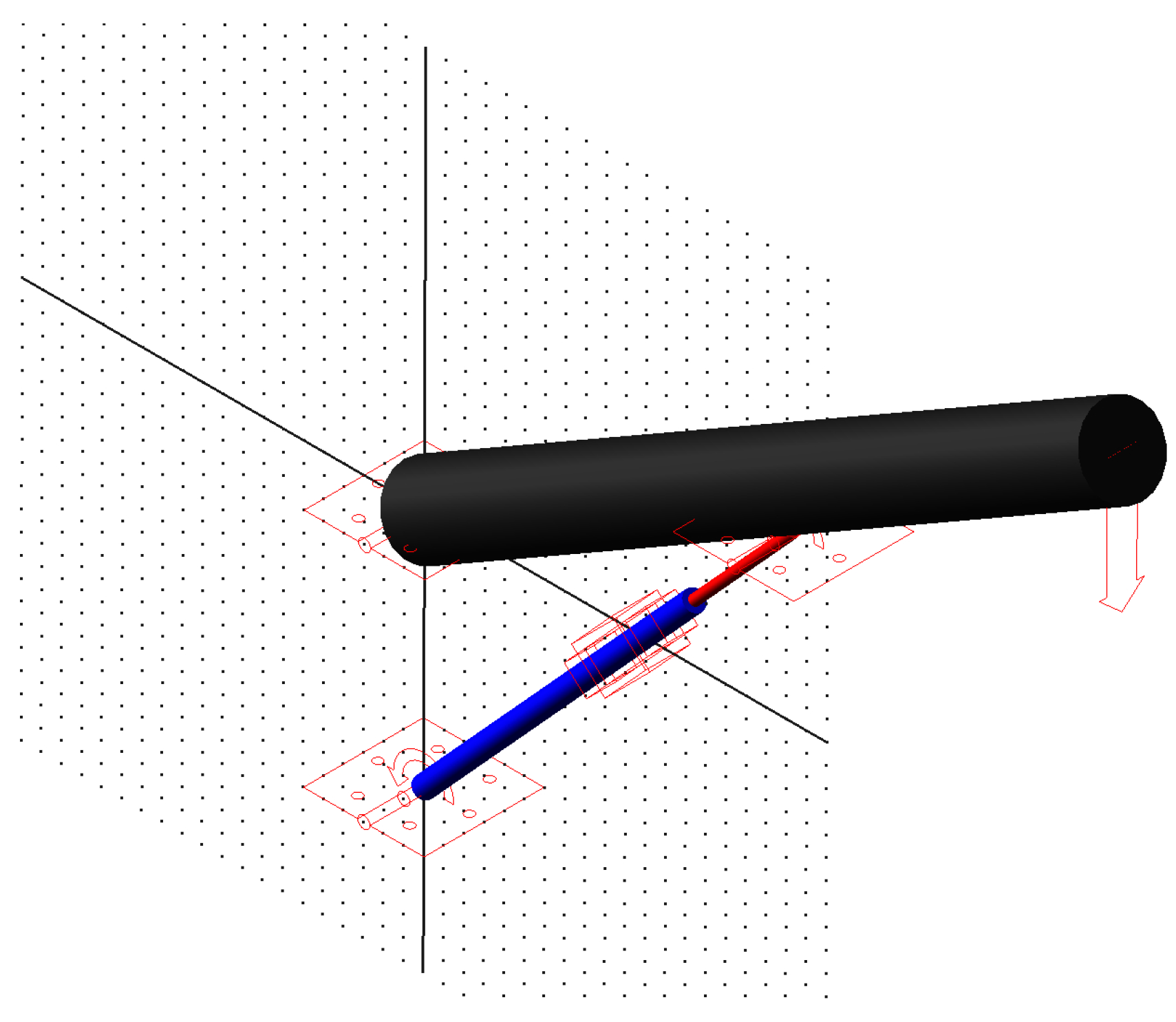
2.1.2. Equations Related to the Mechanical System

A simple mechanical system is introduced in this research, as shown in Figure 3. The rotational movement of the cylindrical beam is driven by the extension or retraction of the hydraulic cylinder. The gravity of the load mass, $G_l$, is applied to the end of the beam, and the entire mechanical system is under the effects of an ocean current with a velocity of $v_{oc}$.

Both the self-rotation of the solid part and the effect of the ocean current cause additional hydrodynamic loads. For a rotating cylinder, the hydrodynamic torque caused by its own rotation, $M_{hd-r}$, and the hydrodynamic torque caused by the ocean current, $M_{hd-oc}$, are as follows [19]:

$$M_{hd-r}=\frac{1}{8}{\rho }_s{C}_D{D}_c\omega \left|\omega \right|\left(l_2^4-l_1^4\right)+\frac{1}{12}{\rho }_s{C}_M\pi D_c^2·\frac{d\omega }{dt}·\left(l_2^3-l_1^3\right),$$

(15)

$$M_{hd-oc}=\frac{1}{2}{\rho }_s{C}_D{D}_c{v}_{oc}\left|v_{oc}\right|{sin}^2\theta \left(l_2^2-l_1^2\right)+\frac{1}{8}{\rho }_s{C}_M\pi D_c^{2}sin\theta ·\frac{d{v}_{oc}}{dt}·\left(l_2^2-l_1^2\right).$$

(16)

where ${\rho }_s$ denotes the density of the seawater, $C_D$ and $C_M$ denote the drag coefficient and inertia coefficient, respectively, $D_c$ denotes the cylinder diameter, $l_1$ and $l_2$ denote the distances from the two ends of the cylinder to the rotation axis, respectively, $\omega$ denotes the angular velocity of the cylinder, $\theta$ denotes the inclination angle of the cylinder, and $v_{oc}$ denotes the velocity of the ocean current.

Equations (15) and (16) are deduced based on Morrison’s equation [31]. With Equations (15) and (16), the hydrodynamic loads can be applied to both the hydraulic cylinder and the cylindrical beam.

2.2. Control Strategy

In a conventional VCHCS, in which a fixed displacement pump and a regular relief valve are used, the output flow of the pump is set to be greater than the maximum flow required by the system. Due to the pressure losses of the valve and pipeline together with the load pressure, the cracking pressure of the relief valve is usually set relatively high to ensure the flow of hydraulic oil, and eventually the movement of the hydraulic cylinder. However, in most cases, the system will not be operating at maximum flow, so the excess flow will return to the oil tank through the relief valve, leading to a lot of energy waste.

From the above analysis, it can be known that there are two solutions to reduce the energy consumption of the deep-sea VCHCS: Reducing the output flow of the power unit and reducing the output pressure of the power unit. For the solution of reducing the flow, a variable-displacement pump or a variable-speed motor is needed. However, either variable-displacement pumps or variable-speed motors respond too slowly [20] to meet the deep-sea VCHCS’s need for rapid response. The ambient pressure in the deep sea will greatly change the viscosity of the hydraulic oil. The pressure loss in the slender pipeline will also change. Then it can be known that the method of adjusting the pressure is more suitable for the deep-sea VCHCS. In the energy-saving control scheme adopted in this research, a proportional relief valve is used to achieve the function of adjusting the output pressure of the power unit, as shown in Figure 1. In addition to the proportional relief valve, two pressure sensors are also configured on the two ports of the hydraulic cylinder. The energy-saving control strategy of the variable pressure scheme, together with the position control strategy, is designed as follows.

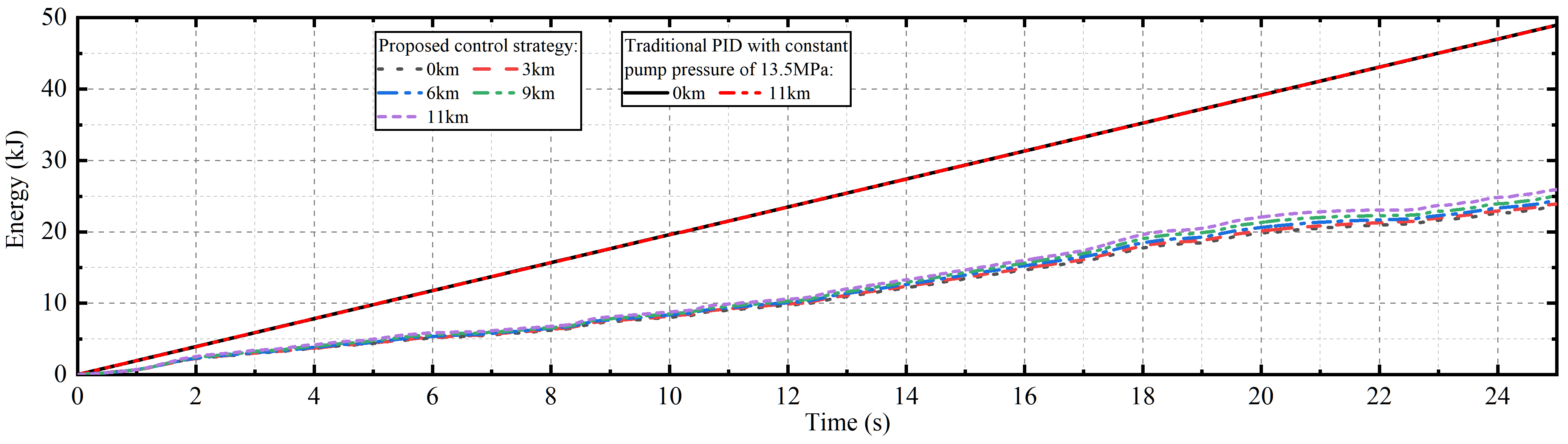
2.2.1. Energy-Saving Control

On the basis of satisfying the pressure required for the movement of the hydraulic cylinder, the smaller the output pressure of the power unit, the more energy-efficient the system is. When the hydraulic cylinder is expected to perform an extension movement, the pressure $P_1$ detected by the pressure sensor is the combined manifestation of the external load and all pressure losses of hydraulic oil flowing from the hydraulic cylinder back to the tank. When extending, the desired velocity of the hydraulic cylinder, ${\dot{x}}_d$, is greater than or equal to 0. Because the hydraulic cylinder’s effective area is $A_1$, the desired flow rate, $Q_d$, is

$$Q_d=A_1{\dot{x}}_d.$$

(17)

With Equations (9) and (17), the estimated pressure loss in the slender pipeline is

$$\Delta P_{pipe}=-\frac{1}{\alpha }ln(1-\frac{128\alpha {\eta }_{0}L{A}_1{\dot{x}}_d{e}^{\alpha P_1}}{\pi D^4}).$$

(18)

With Equations (4), (6) and (17), the estimated pressure loss in the servo valve is

$$\Delta P_{valve}=\frac{A_1^2{\dot{x}}_d^2}{k_q{k}_{sv}u}=\frac{A_1^2{\dot{x}}_d^2}{k_q{k}_{sv}k{u}_{rated}}.$$

(19)

The input current of the servo valve, u, changes at any time according to the position feedback control. To facilitate estimation of the pressure loss in the servo valve, u is replaced with $k{u}_{rated}$ in Equation (19). k is a constant between 0 and 1, and $u_{rated}$ is the rated input current. In this case, for the same desired flow, $Q_d$, or desired velocity, ${\dot{x}}_d$, the larger the constant k is, the smaller the pressure loss in the servo valve is, and the more energy-efficient the system is.

According to Equations (18) and (19), when ${\dot{x}}_d\ge 0$, the desired pump pressure $P_{pd}$ is

$$P_{pd}=P_1-\frac{1}{\alpha }ln(1-\frac{128\alpha {\eta }_{0}L{A}_1{\dot{x}}_d{e}^{\alpha P_1}}{\pi D^4})+\frac{A_1^2{\dot{x}}_d^2}{k_q{k}_{sv}k{u}_{rated}}+P_m,{\dot{x}}_d\ge 0.$$

(20)

where $P_m$ denotes a safety margin to accommodate pressure fluctuations caused by unknown disturbances and uncertainties in the system.

When the hydraulic cylinder is expected to perform a retraction movement, namely when ${\dot{x}}_d<0$, similarly to the above procedure, the desired pump pressure can be derived and then expressed as follows.

$$P_{pd}=P_2-\frac{1}{\alpha }ln(1-\frac{128\alpha {\eta }_{0}L{A}_2{\dot{x}}_d{e}^{\alpha P_2}}{\pi D^4})+\frac{A_2^2{\dot{x}}_d^2}{k_q{k}_{sv}k{u}_{rated}}+P_m,{\dot{x}}_d<0.$$

(21)

The cracking pressure of the proportional relief valve equals the difference between the pump pressure and the tank pressure. Due to the function of the pressure compensator, the tank pressure, $P_t$, is basically the same as the ambient pressure, $P_{am}$. Therefore, the control current applied to the proportional relief valve solenoid is

$$u_{rv}=\frac{P_{pd}-P_{am}}{k_{prv}}.$$

(22)

where $k_{prv}$ denotes the input gain of the proportional relief valve.

As aforementioned, the pump pressure and the corresponding proportional relief valve control signal are preliminarily deduced. However, due to the limitation of rated current and rated cracking pressure of the relief valve, some problems occur under certain extreme conditions. As shown by the black curve in Figure 4, the hydraulic cylinder is expected to linearly extend a certain distance in only 0.1 s. Outside of this short period of 0.1 s, the hydraulic cylinder position is expected to remain unchanged. Due to the extremely short time of 0.1 s, the desired velocity, ${\dot{x}}_d$, is extremely large. Then $P_{pd}$ estimated according to Equation (20) and $u_{rv}$ obtained according to Equation (22) are also very large. When $u_{rv}$ exceeds the rated current of the proportional relief valve, only the rated current can be allowed, and then only the maximum cracking pressure can be provided. In this case, the pump pressure actually provided is less than the required, and a delay inevitably occurs within the 0.1 s of the expected extension. After this short period of 0.1 s, the situation is even worse. Since ${\dot{x}}_d=0$, the second and third terms in Equation (20) are both 0, which means that the actual pump pressure supplied is less than before, and the delay becomes more serious, as shown by the red dotted curve in Figure 4. Obviously, if the proportional relief valve can work at the maximum cracking pressure, x can respond much more quickly than the current situation when ${\dot{x}}_d=0$. The above analysis is based on the example of linear rapid extension. Similar significant delays will also occur in other cases where $\left|{\dot{x}}_d\right|$ is extremely large.

Aiming at the above problem, we designed the following error-related compensation term for the pump pressure.

$$P_{pd-c}=\left\{\begin{array}{c}0,\left|e\right|<e_1\hfill \\ \frac{\left|e\right|-e_1}{e_2-e_1}\times \left(P_{rv-max}-P_{set}\right)+P_{set},e_1\le \left|e\right|<e_2\hfill \\ P_{rv-max},\left|e\right|\ge e_2\hfill \end{array}\right..$$

(23)

where $P_{pd-c}$ denotes the error-related compensated pump pressure, e denotes the error, $e_1$ and $e_2$ denote the error thresholds, $P_{set}$ denotes an artificially set pressure, and $P_{rv-max}$ denotes the maximum cracking pressure of the proportional relief valve.

According to Equation (23), the error-related compensated pump pressure, $P_{pd-c}$, is 0 when the error $\left|e\right|$ is less than $e_1$, which is an allowable smaller error threshold. When $\left|e\right|\ge e_2$, $P_{pd-c}$ is directly set to the maximum cracking pressure of the relief valve, $P_{rv-max}$, since an error larger than the set $e_2$ has seriously affected the position accuracy. When $\left|e\right|$ is between $e_1$ and $e_2$, the value of $P_{pd-c}$ increases linearly from $P_{set}$ to $P_{rv-max}$.

Finally, the estimation formula of the desired pump pressure, $P_{pd}$, is expressed as follows, and the control current applied to the proportional relief valve is still calculated by Equation (22).

$$P_{pd}=\left\{\begin{array}{c}{P}_1-\frac{1}{\alpha }ln(1-\frac{128\alpha {\eta }_{0}L{A}_1{\dot{x}}_d{e}^{\alpha P_1}}{\pi D^4})+\frac{A_1^2{\dot{x}}_d^2}{k_q{k}_{sv}k{u}_{rated}}+P_m+P_{pd-c},{\dot{x}}_d\ge 0\hfill \\ P_2-\frac{1}{\alpha }ln(1-\frac{128\alpha {\eta }_{0}L{A}_2{\dot{x}}_d{e}^{\alpha P_2}}{\pi D^4})+\frac{A_2^2{\dot{x}}_d^2}{k_q{k}_{sv}k{u}_{rated}}+P_m+P_{pd-c},{\dot{x}}_d<0\hfill \end{array}\right..$$

(24)

2.2.2. Position Control

With the advantages of simplicity, practicality, and so on, the PID (Proportional-Integral-Derivative) control algorithm is widely utilized in automatic control. The control parameters in the traditional PID algorithm are constants, makes it unsuitable for applications with high accuracy requirements and large changes in system parameters. Nowadays, researchers have developed various variable-gain PID control algorithms to improve its control performance. Among them, fuzzy control [32,33], artificial neural network [34,35], fractional-order calculus [36,37], etc., are all used to optimize the PID algorithm. The hydraulic oil viscosity and pipeline pressure loss in the deep-sea VCHCS vary greatly at different depths; that is, the operating parameters of the system itself vary greatly. Therefore, the traditional PID algorithm cannot guarantee the consistency of the control accuracy of the deep-sea VCHCS at different depths, and a variable-gain PID control algorithm is needed.

Subsea equipment usually carries a large number of actuators, and the computing power that can be allocated to the deep-sea VCHCS is limited. Therefore, it is desirable to use a control algorithm that is simple, reliable and easy to implement. In this research, a variable-gain PID control algorithm, which is described as follows, is designed to achieve precise position control of the deep-sea VCHCS and accuracy consistency at different working depths.

$$U=k_{p}e+k_i\int edt+k_d\frac{de}{dt},$$

(25)

$$k_p=k_1+k_2{e}^2.$$

(26)

where U denotes the controller output, e denotes the error, $k_p$, $k_i$, $k_d$ denote the proportional gain, the integral gain, and the differential gain, respectively, $k_1$ and $k_2$ are constants.

From the above two equations, it can be known that $k_i$ and $k_d$ are constants, and the proportional gain $k_p$ is a function of e. When $\left|e\right|$ becomes smaller and tends to 0, $k_p$ also becomes smaller and tends to $k_1$, which helps reduce overshoot. When $\left|e\right|$ gets larger, $k_p$ increases, and the system responds faster to reduce the error.

3. Model

3.1. Model and Settings

Based on the fundamental equations and control strategy in the previous section, a co-simulation model of the deep-sea VCHCS is built in the AME Sim and ADAMS platforms. Figure 5 shows the hydraulic system model and control model established in AME Sim. Figure 6 shows the mechanical system model established in ADAMS. The force signal is transmitted from AME Sim to ADAMS, while the position and velocity signals are transmitted from ADAMS to AME Sim.

The AME Sim model shown in Figure 5 is consistent with the schematic diagram shown in Figure 1. Among them, the PID controller adopts the module that comes with the software, the gains $k_i$ and $k_d$ are constants, and the gain $k_p$ is variable. The energy-saving control strategy proposed in Section 2.2.1 and the $k_p$ change rule described in Equation (26) are encapsulated in the module named “Controller” in Figure 5. The control parameters of variable gain PID and energy saving strategy are listed in

Table 1. Control parameters.

Object	Parameter	Symbol	Value
Position control	Proportional gain	$k_p$	4 + 0.5 × 10${}^{-2}$
	Integral gain	$k_i$	0.001
	Derivative gain	$k_d$	0.005
Energy-saving control	Error thresholds	$e_1$, $e_2$	2.5, 5
	Artificially set pressure	$P_{set}$	20 MPa
	User-defined constant	k	0.7
	Safety margin pressure	$P_m$	1 MPa

. The ADAMS model shown in Figure 6 is consistent with the mechanical system shown in Figure 3. Hydrodynamic loads are applied to each moving part according to Equations (15) and (16). The parameter settings in the co-simulation model are listed in Appendix B. The ambient pressure increases by 10 MPa for each 1 km increase in depth. The Mariana Trench is approximately 11 km below sea level at its deepest point, with a maximum ambient pressure of 110 MPa. The simulation step and convergence tolerance are 0.001 s and $1\times {10}^{-5}$, respectively. The simulation type is dynamic, and the solver type in AME Sim is regular. More details about the co-simulation model can be found in [19].

When building the control strategy model, some issues need to be carefully dealt with. According to Equation (24), it can be known that the estimated required pump pressure is switched according to whether ${\dot{x}}_d<0$. Obviously, instantaneous and abrupt switching can cause system instability. AME Sim provides a smooth switching method, and the equation is expressed as follows.

$$Output=\left\{\begin{array}{c}\gamma \times Input1+\left(1-\gamma \right)\times Input2,Switchcommand\ge Switchthreshold\hfill \\ \left(1-\gamma \right)\times Input1+\gamma \times Input2,Switchcommand<Switchthreshold\hfill \end{array}\right..$$

(27)

where $\gamma$ is a time-varying coefficient between 0 and 1.

When it is not in the transition period, $\gamma$ equals 1. If the switch command is greater or equal to the switch threshold, the output equals the input 1. If the switch command is less than the switch threshold, the output equals the input 2. When it is in the smooth transition process, $\gamma$ changes with time, so that the output switches smoothly between input 1 and input 2. The value of $\gamma$ is automatically adjusted by the software according to the transition duration set by the user. In the model established in this research, the transition duration is set to 0.1s.

Besides, when $x_d$ remains unchanged, due to the numerical calculation accuracy of the differentiator in the software, ${\dot{x}}_d$ is not exactly 0, but a changing value with an extremely tiny absolute value, which may be positive or negative. This can result in the pump pressure constantly switching and therefore causing system instability. To avoid this problem, the switch threshold of ${\dot{x}}_d$ in the model is adjusted from 0 to –0.01.

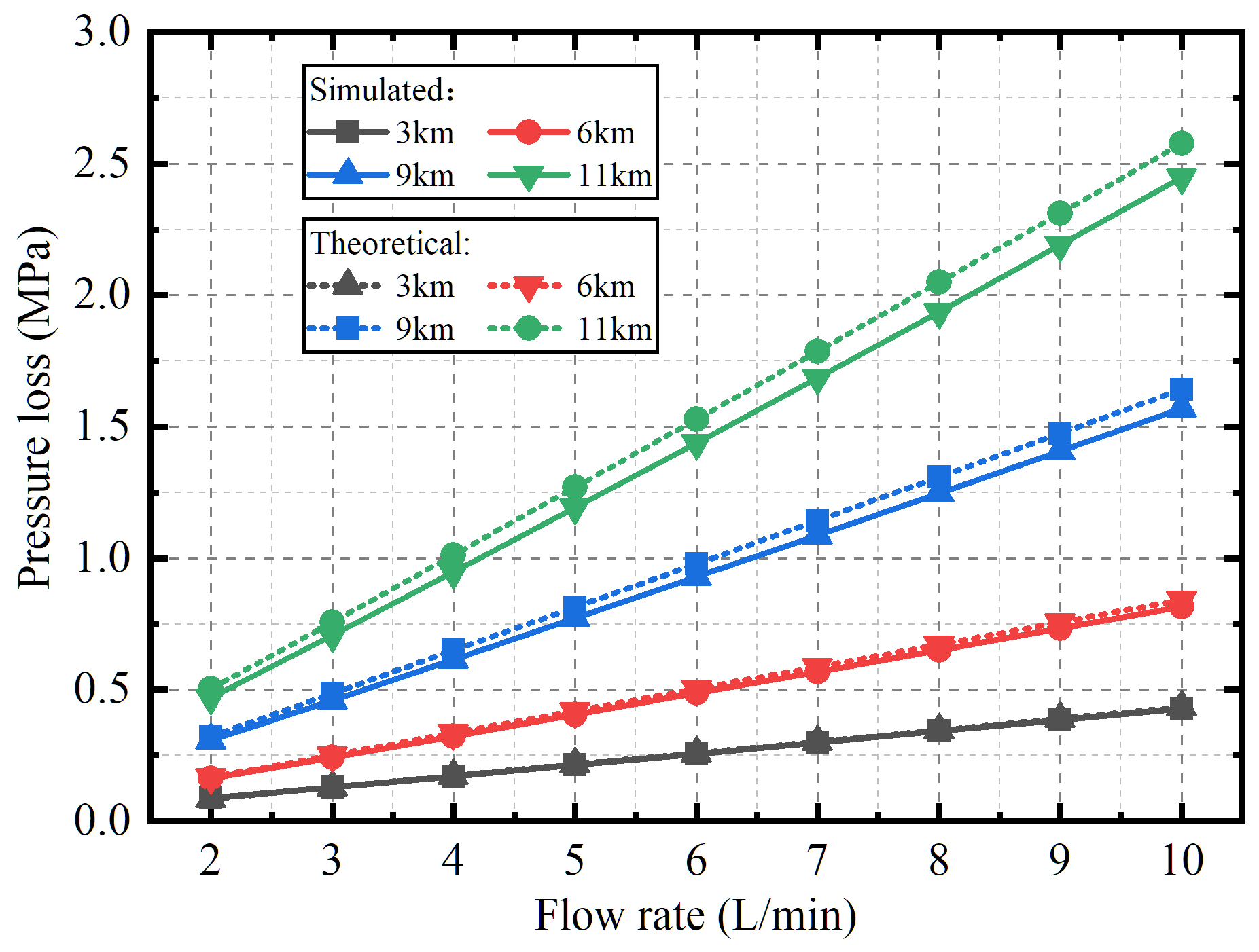
3.2. Validation of Pipeline Pressure Loss

In the model established in this study, the novel formula expressed by Equation (9) is used to calculate the pipeline pressure loss, and this formula is also used in the energy saving control strategy described in Section 2.2.1. Therefore, it is necessary to ensure that the pipeline pressure loss obtained by the simulation is consistent with Equation (9). Figure 7 depicts the simulated pipeline pressure loss in a single slender pipeline at different depths together with theoretical values calculated by Equation (9). It shows that the simulated pipeline pressure loss is consistent with the theoretical value at different depths and different flow rates. Among them, the maximum error is –6.7% compared with the theoretical value. Figure 7 also shows that the pipeline pressure loss varies greatly at different subsea depths, which has significant influence on the working performance and energy efficiency of the deep-sea VCHCS at different depths. The working performance and the energy efficiency of the deep-sea VCHCS are just what the proposed control strategy in this research is supposed to deal with.

4. Results and Discussions

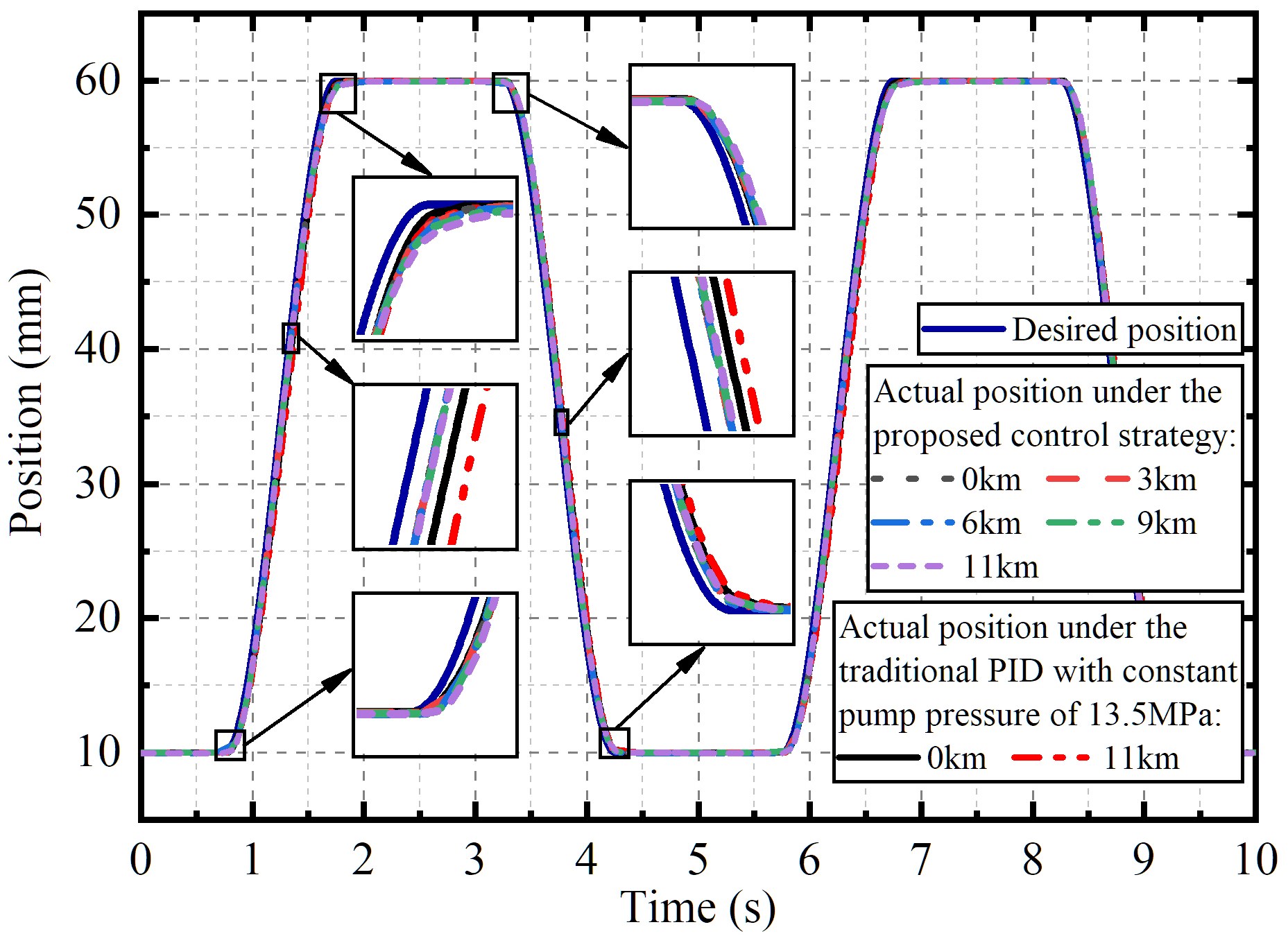
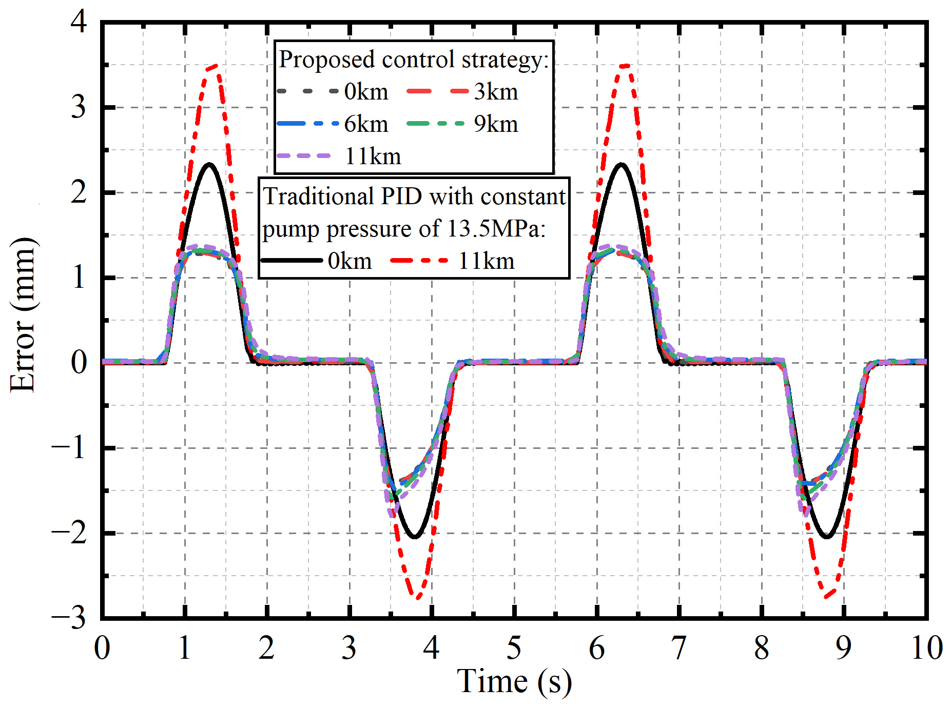
4.1. Multi-Step Movement

Figure 8 depicts the tracking performance of the deep-sea VCHCS at different depths in the sea while performing a multi-step movement, and Figure 9 shows the corresponding tracking errors. As a comparison, the results with traditional PID control and constant pump pressure are also plotted in the figures. It can be known from Figure 9 that the control strategy proposed in this research has better control accuracy compared with the traditional PID control combined with constant pump pressure when performing the multi-step motion. In addition, the proposed control strategy also presents the advantage that the control accuracy is basically the same under different working depths.

Figure 10 and Figure 11 depict the pump pressure and the energy consumption of the deep-sea VCHCS at different depths in the sea while performing a multi-step movement. It can be known from Figure 10 that the proposed control strategy realizes the adaptive adjustment of pump pressure. The variations in pump pressure at different working depths are consistent with each other. The deeper the depth in the sea is, the greater the pump pressure is. This is due to the increase in the viscosity of the hydraulic oil caused by the ambient pressure and, subsequently, the increase in the pipeline pressure loss. Since the pump pressure can be adjusted adaptively, the proposed control strategy also realizes the energy saving of the deep-sea VCHCS, as shown in Figure 11. When compared to traditional PID control with 13.5 MPa pump pressure, the proposed strategy can save energy by 43% on land and 36.5% at 11 km depth in the sea.

For the tracking errors shown in Figure 9 and the pump pressures shown in Figure 10, when the position increases, the shape of the curves is different from that when the position decreases. There is even a small overshoot in the pump pressure curve when the position starts decreasing and ends decreasing. The abovementioned phenomenon occurs for the following two reasons. First, as can be seen from Figure 3, both the mechanical system’s gravity and the external load tend to make the hydraulic cylinder retract, so they are a hindrance when the hydraulic cylinder position increases, but a benefit when the hydraulic cylinder position decreases. Another reason is that the effective working area of the two chambers in the hydraulic cylinder is different. The above two reasons make the pressure when the position increases different from that when it decreases. According to Equation (24), the desired pump pressure switches based on whether the desired velocity is less than 0, that is, the switching occurs when the desired position begins to decrease or ends to decrease. Therefore, due to the aforementioned two physical structural reasons, the pump pressure inevitably undergoes abrupt changes during switching, and then overshoot occurs. Further, due to the change in pump pressure, the drive capability of the system changes. Then the tracking performance when the position increases is different from when it decreases, leading to the shape change of error curves. Similar phenomena also exist in the tracking error and the pump pressure in the rest results, and the reason is the same, so it will not be repeated in the following.

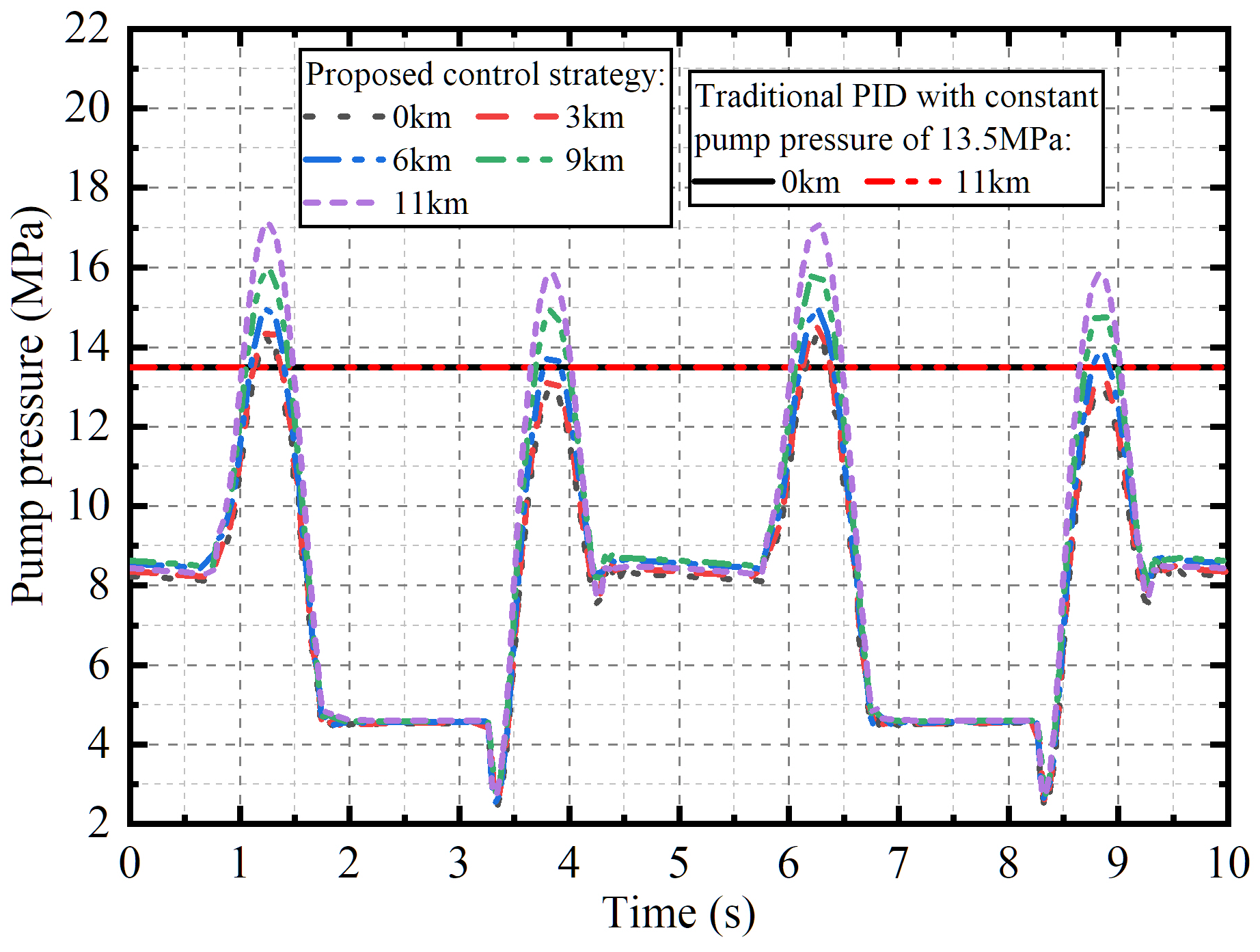
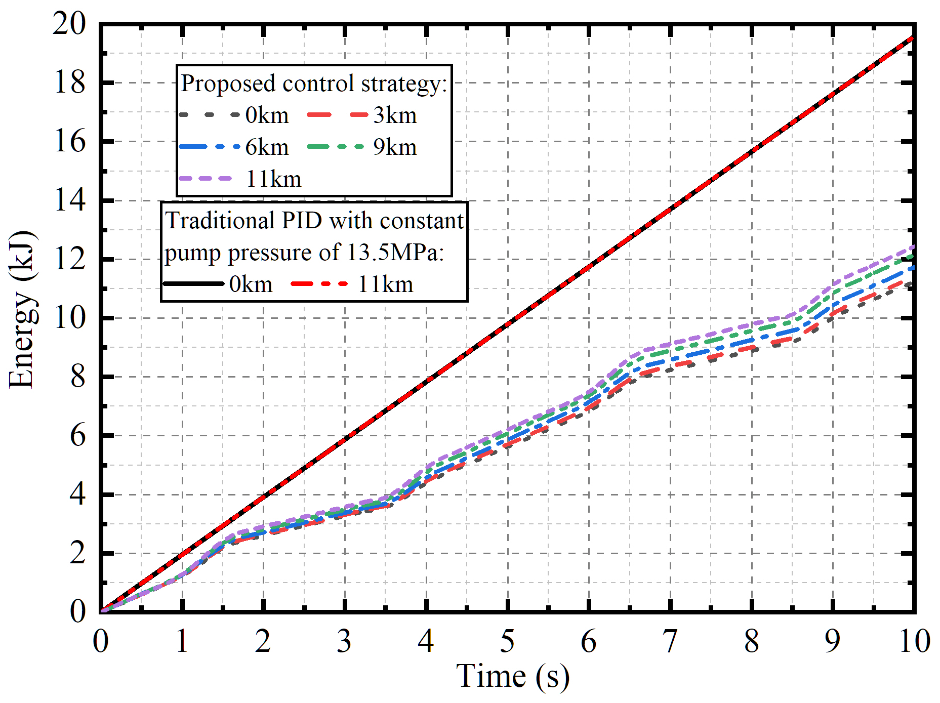
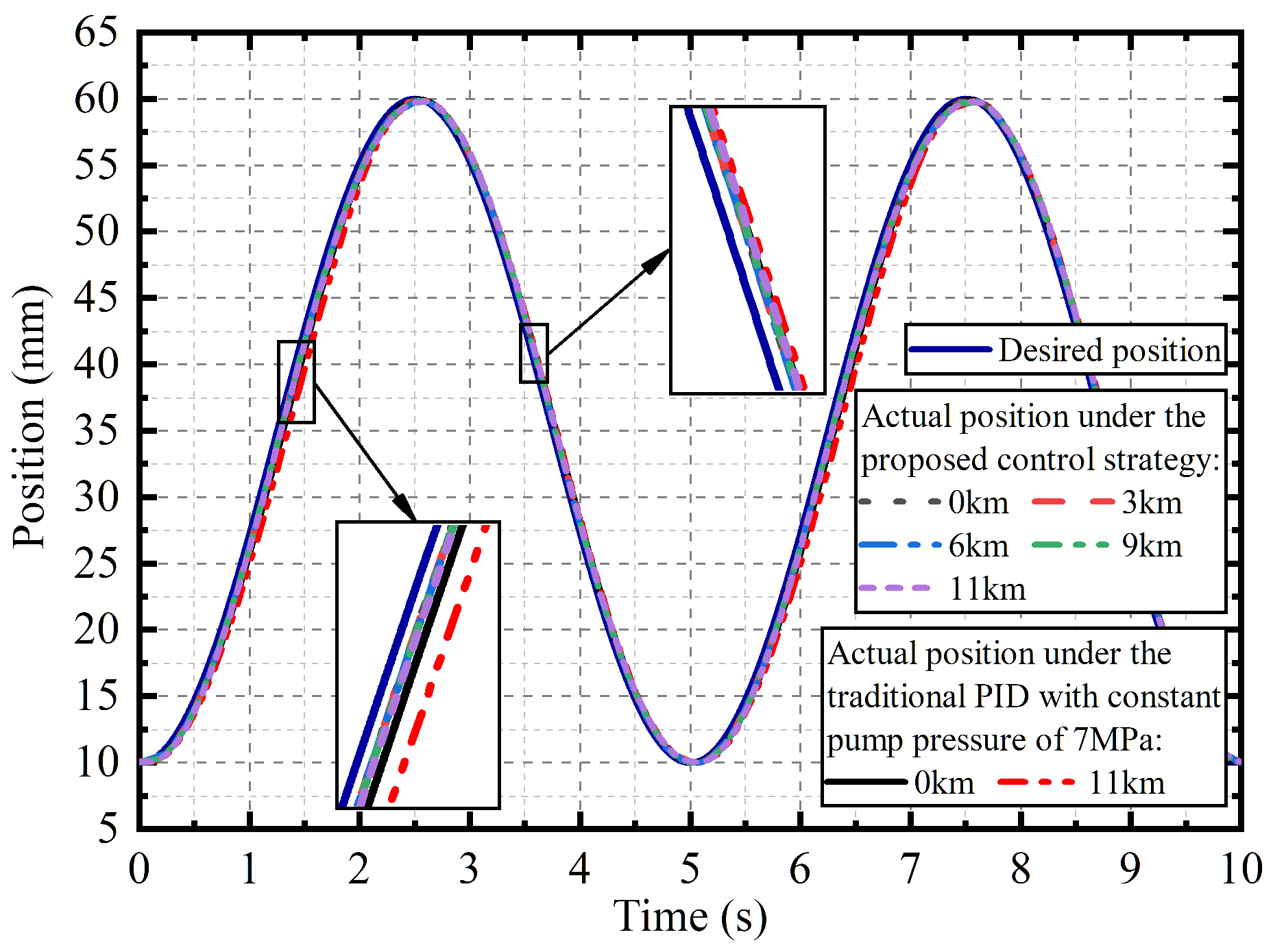
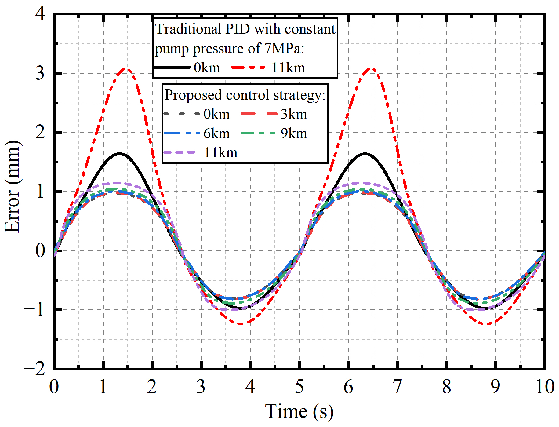
4.2. Harmonic Movement

When the deep-sea VCHCS performs a harmonic movement, the tracking performance, the tracking error, the pump pressure, and the energy consumption are plotted in Figure 12, Figure 13, Figure 14 and Figure 15, respectively. It can be known from Figure 12, Figure 13, Figure 14 and Figure 15 that the proposed control strategy also presents the same advantages when performing a harmonic movement as when performing a multi-step movement in the previous subsection. That is, it has better control accuracy, basically the same performance at different depths, variable pump pressure, and less energy consumption. When compared to traditional PID control with 7 MPa pump pressure, the proposed strategy can save energy by 36% on land and 30% at 11 km depth in the sea.

4.3. Complex Movement

A complex movement simulation is also performed in this research. As shown in Figure 16, the complex movement includes random movement, multi-step movement, harmonic movement, and ramp movement. It can be known from Figure 16, Figure 17 and Figure 18 that the proposed control strategy also presents the same advantages, such as better control accuracy, basically the same performance at different depths, and less energy consumption. When compared to traditional PID control with 13.5 MPa pump pressure, the proposed strategy can save energy by 52% on land and 47% at 11 km depth in the sea.

It should be noted that the tracking error of the proposed control strategy is slightly larger than that of the traditional PID combined with the constant pump pressure at around 2.8 s and 4.3 s in Figure 17. This can also be seen from the enlarged view of around 2.8 s in Figure 16. The reason for this phenomenon is explained as follows. It can be seen from Figure 16 that the desired positions at these two time points increase relatively slowly, that is, the desired velocity ${\dot{x}}_d$ is relatively small. Therefore, according to Equation (24), the pump pressure of the system is also smaller at this time. In the case of traditional PID combined with constant pump pressure, the pump pressure is constant at 13.5 MPa, which is much larger than that in the proposed control strategy. This means that its driving ability is stronger at this time, which leads to better tracking performance. Of course, more energy is consumed at the same time. While the tracking performance of the proposed control strategy is slightly weaker in these two time periods, it can be seen from Figure 17 that the tracking error is less than 1mm, which is acceptable.

4.4. Other Performance

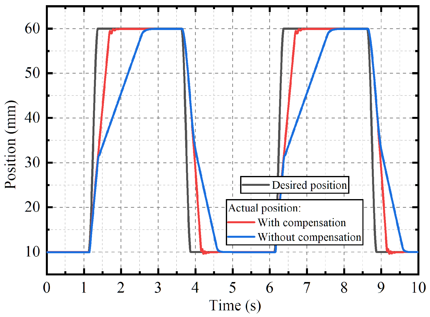
4.4.1. Error-Related Pump Pressure Compensation

As described in Section 2.2.1, an error-related compensated pump pressure expressed by Equation (23) is designed to cope with the significant delay shown in Figure 4. Figure 19 plots the tracking performance with or without error-related compensated pump pressure when performing a multi-step movement with an extremely short switching transition at a depth of 11 km in the sea. It can be known from Figure 19 that when the desired position remains unchanged, that is, when the desired velocity is 0, the position output of the deep-sea VCHCS is seriously delayed when there is no compensation, and the tracking performance is significantly improved with the error-related pump pressure compensation.

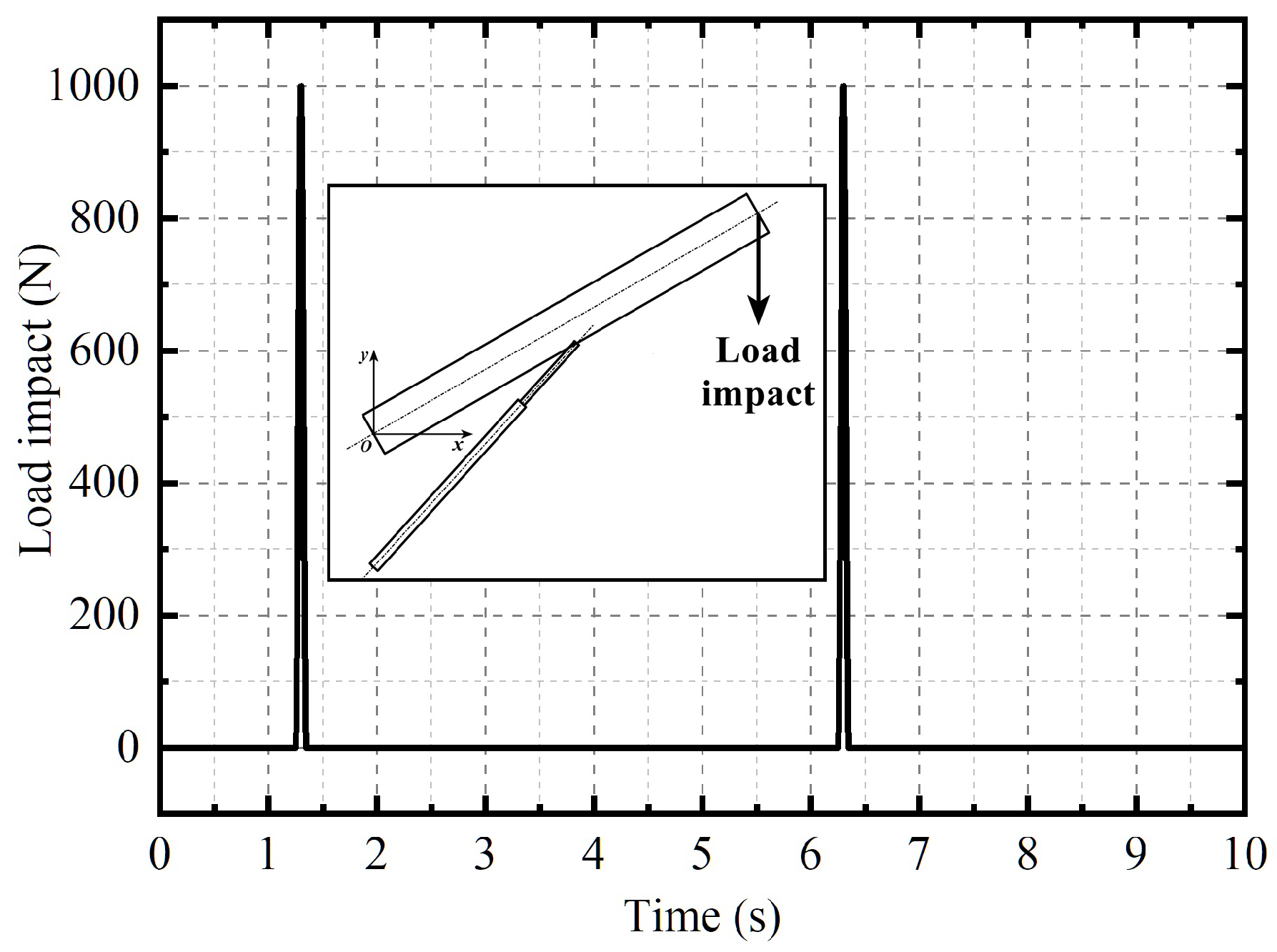
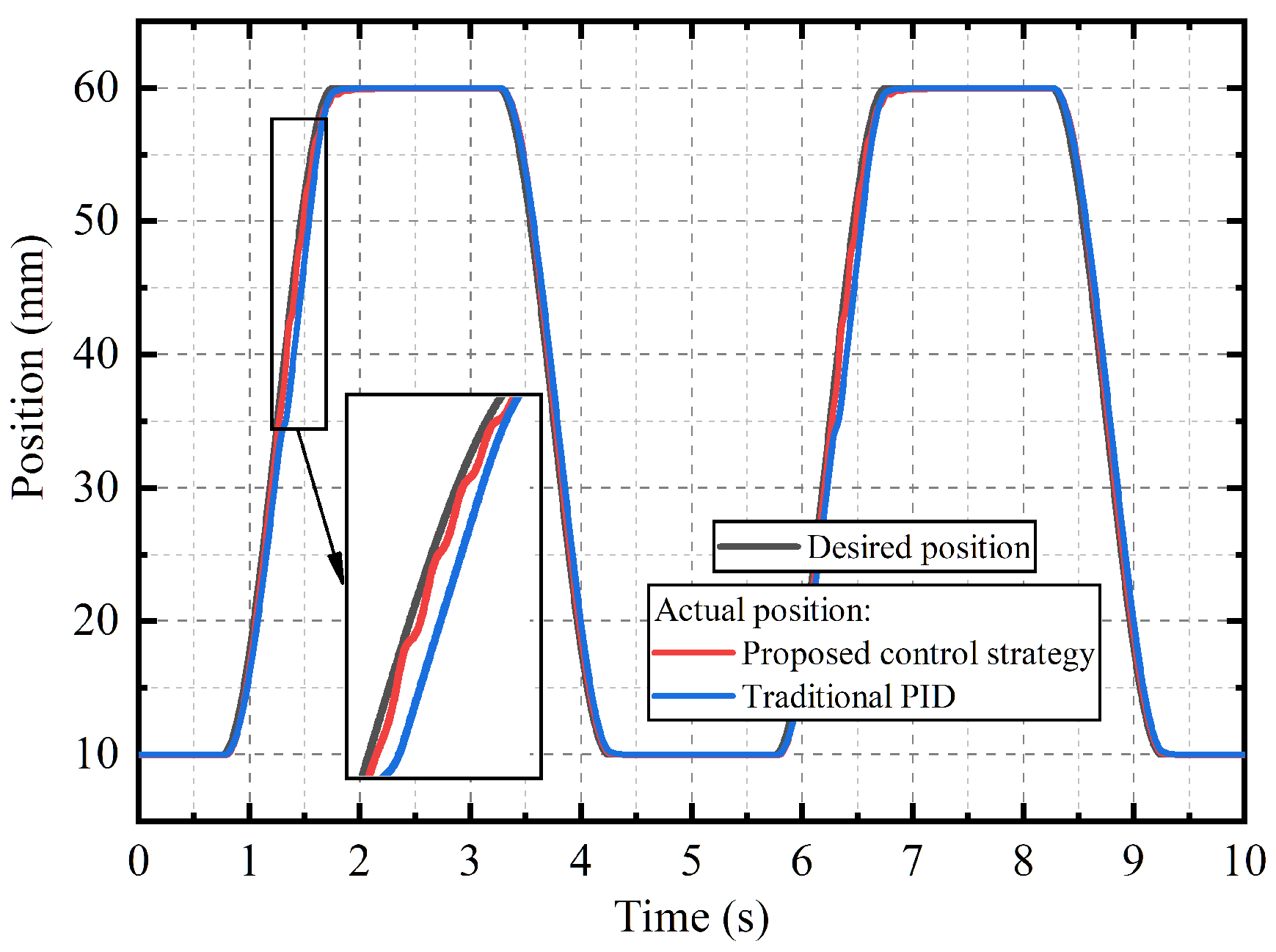
4.4.2. Tracking Performance under Load Impact

Deep-sea VCHCSs will encounter many disturbances during operation, and the most common disturbance is load impact. As shown in Figure 20, the load impact is applied to the end of the cylindrical beam in the mechanical system, and the direction is vertically downward. Figure 20 also shows the time when the load impact occurs. The amplitude of the load impact is 1000 N, and the duration is 0.1 s. Figure 21 and Figure 22 plot the tracking performance and tracking error under the additional sudden load impact when performing a multi-step movement at a depth of 11 km in the sea. Figure 22 clearly shows that the control strategy proposed in this research has good resistance to load impact.

4.5. Parameter Study

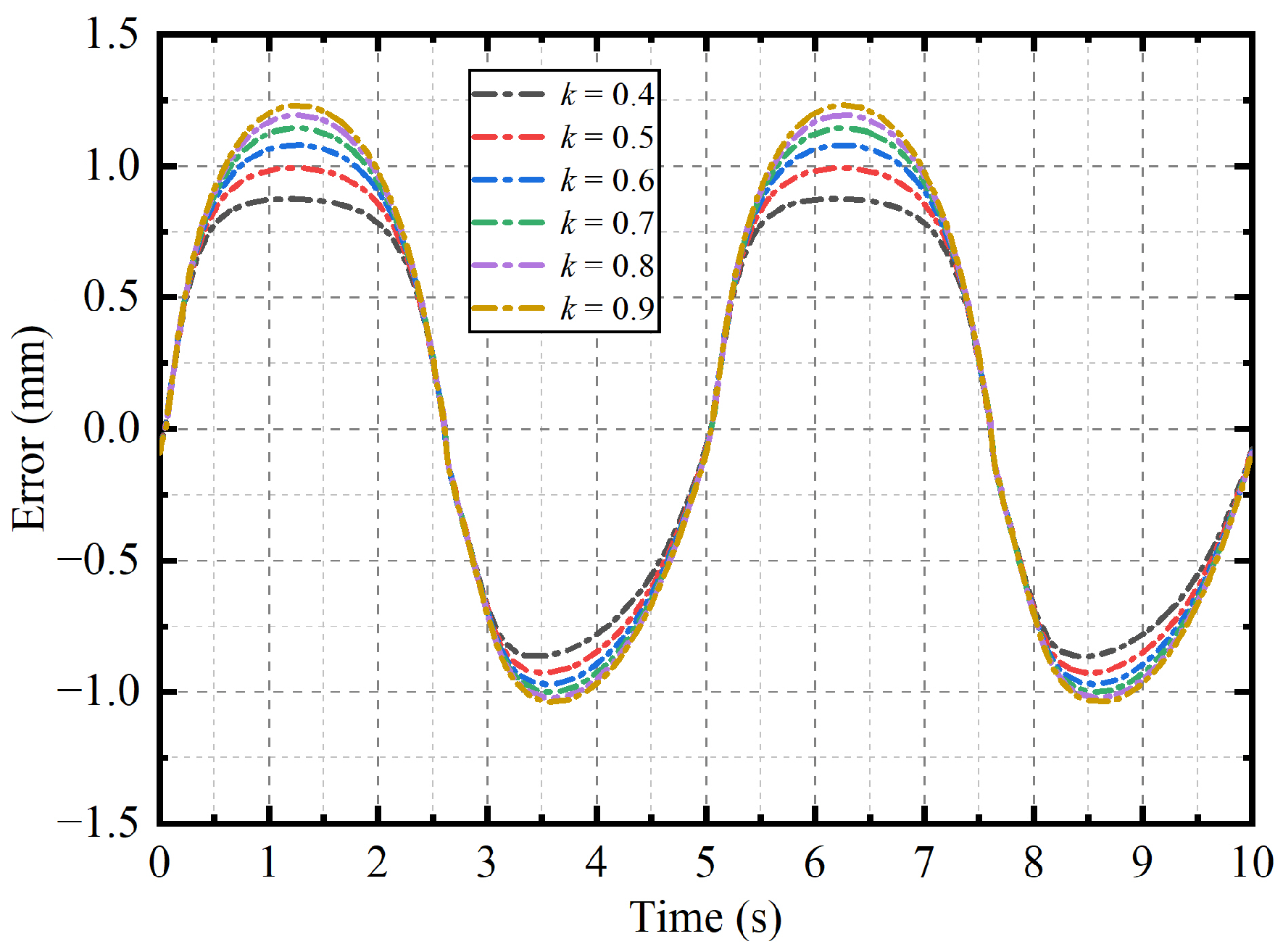
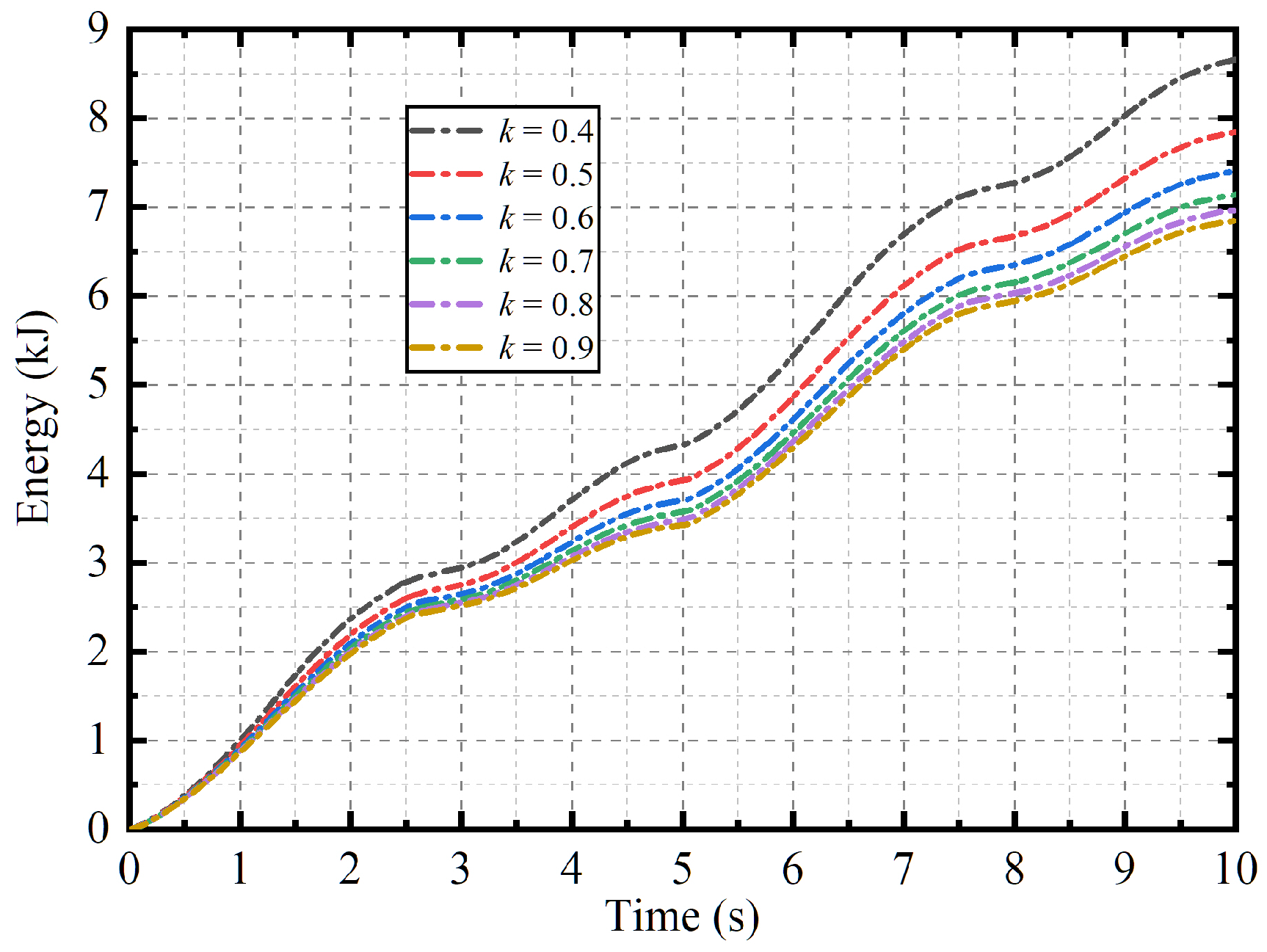
4.5.1. Used-Defined Constant k for Estimating Pressure Loss in Servo Valve

To estimate the pressure loss in the servo valve, Equation (19) introduces a constant k. When performing a harmonic movement at a depth of 11 km in the sea, how k affects the tracking error and the energy consumption of the deep-sea VCHCS is shown in Figure 23 and Figure 24, respectively. According to Figure 23 and Figure 24, it can be known that a larger k can result in lower energy consumption, but also lower control accuracy at the same time. As listed in Table 1, k is set as 0.7 in the model of the deep-sea VCHCS established in this research since it can lead to a balance between energy saving and precise control.

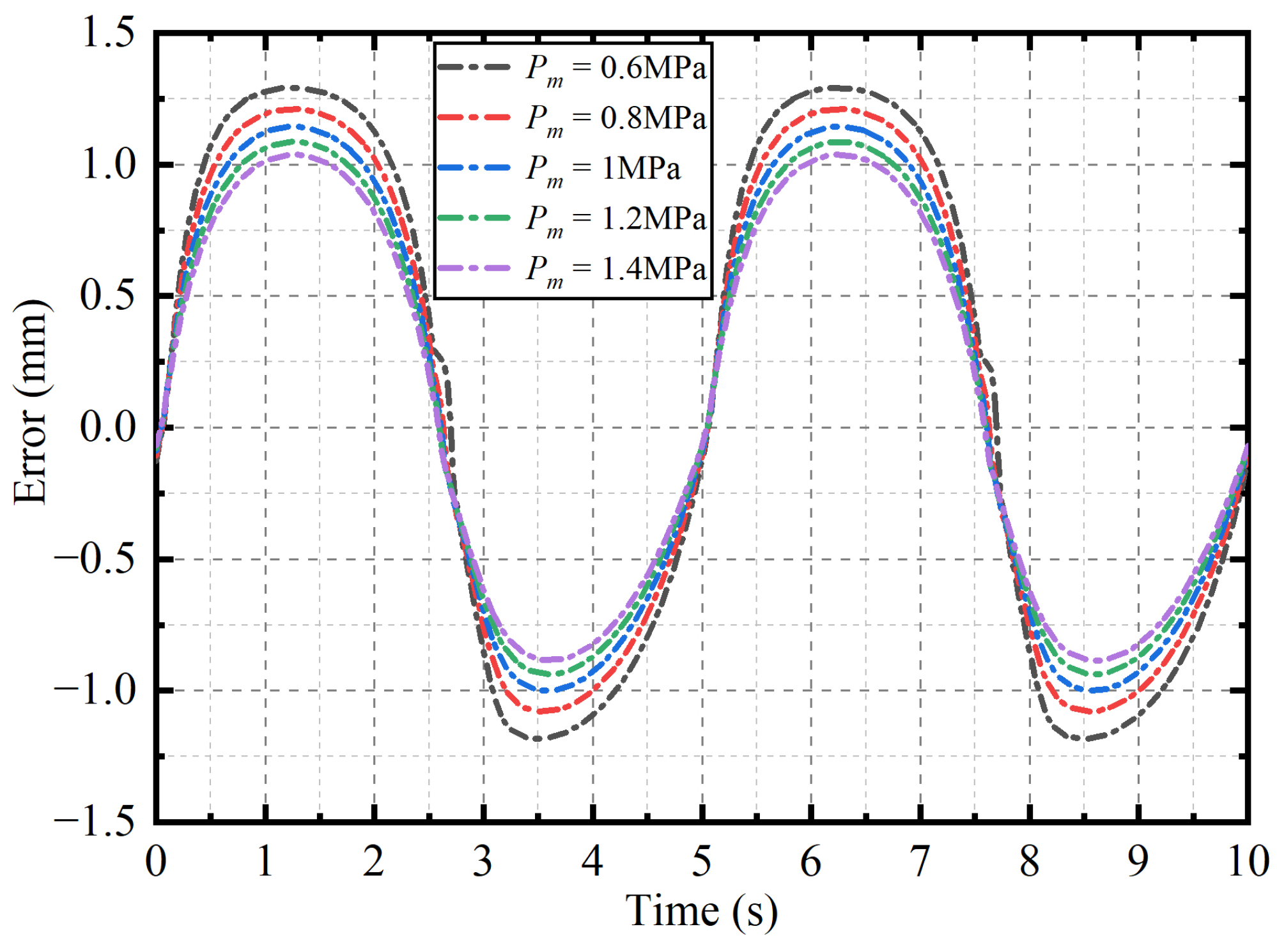
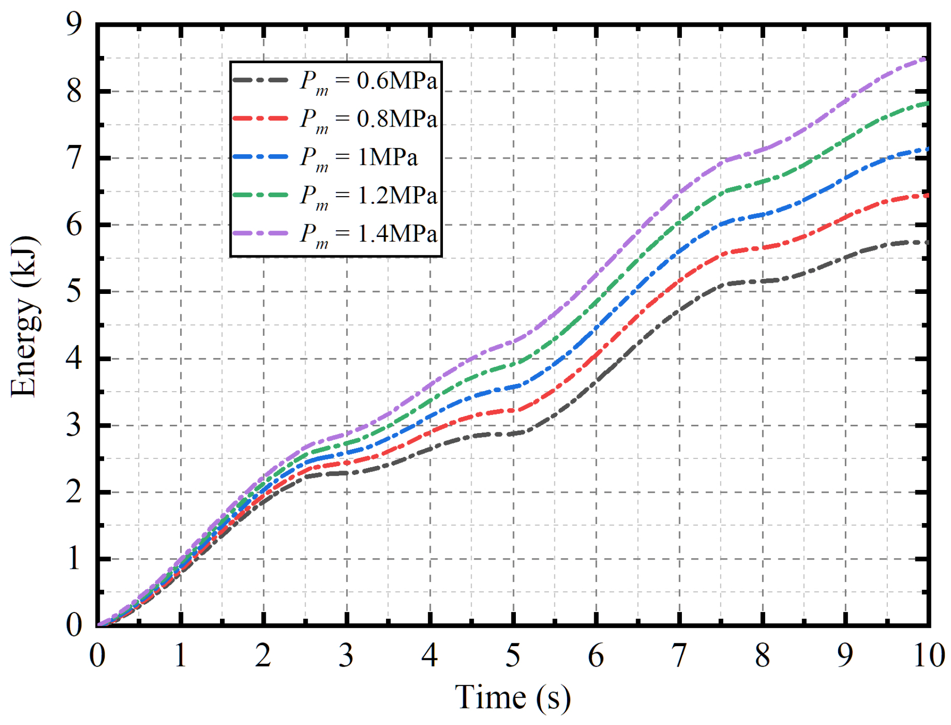
4.5.2. Safety Margin Pressure $P_m$

Safety margin pressure $P_m$ is introduced to tolerate pressure fluctuations caused by unknown disturbances and uncertainties in the deep-sea VCHCS. As shown in Figure 25 and Figure 26, when performing a harmonic movement at a depth of 11 km in the sea, a larger $P_m$ can result in more energy consumption, but also higher control accuracy at the same time. In this research, $P_m$ is set to 1 MPa, as listed in Table 1, and Figure 25 and Figure 26 show that a $P_m$ of 1 MPa can achieve a balance between energy saving and precise control.

5. Conclusions

An energy-saving position control method for deep-sea VCHCS has been proposed in this research. The solution to reducing energy consumption is to adjust the pump pressure according to the operation state of the system with a proportional relief valve. A variable gain PID algorithm is also designed for precision position control. With the AME Sim and ADAMS platforms, a co-simulation model of the deep-sea VCHCS has been established. Simulations of multi-step movement, harmonious movement and complex movement under different depths in the sea have been carried out to verify the effectiveness of the proposed control strategy. The simulation results show that the proposed control strategy can realize the function of adaptively adjusting the pump pressure according to the expected command and working depth. Compared with traditional PID control with a constant pump pressure, the control strategy proposed in this research shows advantages such as lower energy consumption, better control accuracy, better resistance to load impact, and accuracy consistency under different working depths. When working at 11 km depth in the sea, the proposed method is capable of saving energy by 36.5% for the multi-step movement, by 30% for the harmonic movement, and by 47% for the complex movement. A larger user-defined constant k or a smaller safety margin pressure $P_m$ leads to less energy consumption but also lower position accuracy. In summary, the present work in this research provides an effective solution that can realize energy saving and precise control of the deep-sea VCHCS in the wide span of depth in the sea. An important issue to resolve for future studies is experimental tests on real objects, especially under the ambient pressure of 110 MPa, which is equivalent to the seawater ambient pressure at the bottom of the Mariana Trench.

References

1. Lynch, B.; Ellery, A. Efficient Control of an AUV-Manipulator System: An Application for the Exploration of Europa. IEEE J. Ocean. Eng. 2014, 39, 552–570. [Google Scholar] [CrossRef]
2. Sivčev, S.; Rossi, M.; Coleman, J.; Omerdić, E.; Dooly, G.; Toal, D. Collision Detection for Underwater ROV Manipulator Systems. Sensors 2018, 18, 1117. [Google Scholar] [CrossRef] [PubMed] [Green Version]
3. Wang, C.; Zhang, Q.; Zhang, Q.; Zhang, Y.; Huo, L.; Wang, X. Construction and Research of an Underwater Autonomous Dual Manipulator Platform. In Proceedings of the 2018 OCEANS—MTS/IEEE Kobe Techno-Oceans (OTO), Kobe, Japan, 28–31 May 2018; pp. 1–5. [Google Scholar] [CrossRef]
4. Sivčev, S.; Coleman, J.; Omerdić, E.; Dooly, G.; Toal, D. Underwater manipulators: A review. Ocean Eng. 2018, 163, 431–450. [Google Scholar] [CrossRef]
5. Liu, Y.; Wu, D.; Li, D.; Deng, Y. Applications and Research Progress of Hydraulic Technology in Deep Sea. J. Mech. Eng. 2018, 54, 14–23. [Google Scholar] [CrossRef]
6. Wang, F.; Chen, Y. Dynamic characteristics of pressure compensator in underwater hydraulic system. IEEE-ASME Trans. Mechatron. 2014, 19, 777–787. [Google Scholar] [CrossRef]
7. Wu, J.B.; Li, L.; Wei, W. Research on dynamic characteristics of pressure compensator for deep-sea hydraulic system. Proc. Inst. Mech. Eng. Part M J. Eng. Marit. Environ. 2022, 256, 19–33. [Google Scholar] [CrossRef]
8. Liu, Y.; Ren, X.; Wu, D.; Li, D.; Li, X. Simulation and analysis of a seawater hydraulic relief valve in deep-sea environment. Ocean Eng. 2016, 125, 182–190. [Google Scholar] [CrossRef]
9. Liu, Y.; Deng, Y.; Fang, M.; Li, D.; Wu, D. Research on the torque characteristics of a seawater hydraulic axial piston motor in deep-sea environment. Ocean Eng. 2017, 146, 411–423. [Google Scholar] [CrossRef]
10. Li, L.; Wu, J.B. Deformation and leakage mechanisms at hydraulic clearance fit in deep-sea extreme environment. Phys. Fluids 2020, 32, 067115. [Google Scholar] [CrossRef]
11. Ye, Y.; Yin, C.B.; Gong, Y.; Zhou, J.J. Position control of nonlinear hydraulic system using an improved PSO based PID controller. Mech. Syst. Signal Process. 2017, 83, 241–259. [Google Scholar] [CrossRef]
12. Yao, J.; Deng, W.; Sun, W. Precision Motion Control for Electro-Hydraulic Servo Systems With Noise Alleviation: A Desired Compensation Adaptive Approach. IEEE/ASME Trans. Mechatron. 2017, 22, 1859–1868. [Google Scholar] [CrossRef]
13. Won, D.; Kim, W.; Tomizuka, M. Nonlinear Control With High-Gain Extended State Observer for Position Tracking of Electro-Hydraulic Systems. IEEE/ASME Trans. Mechatron. 2020, 25, 2610–2621. [Google Scholar] [CrossRef]
14. Wang, C.; Ji, X.; Zhang, Z.; Zhao, B.; Quan, L.; Plummer, A. Tracking differentiator based back-stepping control for valve-controlled hydraulic actuator system. ISA Trans. 2021, 119, 208–220. [Google Scholar] [CrossRef] [PubMed]
15. Yao, J.; Wang, C. Model reference adaptive control for a hydraulic underwater manipulator. J. Vib. Control 2012, 18, 893–902. [Google Scholar] [CrossRef]
16. Cao, X.; Gu, L.; Luo, G.; Wang, Y. The adaptive robust tracking control of deep-sea hydraulic manipulator based on backstepping design. In Proceedings of the OCEANS 2015—MTS/IEEE Washington, Washington, DC, USA, 19–22 October 2015; pp. 1–6. [Google Scholar] [CrossRef]
17. Zhang, Y.; Zhang, Q.; Zhang, A.; Cui, S.; Du, L.; Huo, L. Experiment research on control performance for the actuators of a deep-sea hydraulic manipulator. In Proceedings of the OCEANS 2016 MTS/IEEE Monterey, Monterey, CA, USA, 19–23 September 2016; pp. 1–6. [Google Scholar] [CrossRef]
18. Tian, Q.; Zhang, Q.; Chen, Y.; Huo, L.; Li, S.; Wang, C.; Bai, Y.; Du, L. Influence of Ambient Pressure on Performance of a Deep-sea Hydraulic Manipulator. In Proceedings of the OCEANS 2019, Marseille, France, 17–20 June 2019; pp. 1–6. [Google Scholar] [CrossRef]
19. Wu, J.B.; Li, L.; Zou, X.L.; Wang, P.J.; Wei, W. Working Performance of the Deep-Sea Valve-Controlled Hydraulic Cylinder System under Pressure-Dependent Viscosity Change and Hydrodynamic Effects. J. Mar. Sci. Eng. 2022, 10, 362. [Google Scholar] [CrossRef]
20. Baghestan, K.; Rezaei, S.M.; Talebi, H.A.; Zareinejad, M. An energy-saving nonlinear position control strategy for electro-hydraulic servo systems. ISA Trans. 2015, 59, 268–279. [Google Scholar] [CrossRef]
21. Lin, T.; Zhou, S.; Chen, Q.; Fu, S. A Novel Control Strategy for an Energy Saving Hydraulic System With Near-Zero Overflowing Energy-Loss. IEEE Access 2018, 6, 33810–33818. [Google Scholar] [CrossRef]
22. Lyu, L.; Chen, Z.; Yao, B. Advanced Valves and Pump Coordinated Hydraulic Control Design to Simultaneously Achieve High Accuracy and High Efficiency. IEEE Trans. Control Syst. Technol. 2021, 29, 236–248. [Google Scholar] [CrossRef]
23. Wang, W.; Du, W.; Cheng, C.; Lu, X.; Zou, W. Output feedback control for energy-saving asymmetric hydraulic servo system based on desired compensation approach. Appl. Math. Model. 2022, 101, 360–379. [Google Scholar] [CrossRef]
24. Tongli, C. Hydraulic Control Systems; Tsinghua University Press: Beijing, China, 2014. (In Chinese) [Google Scholar]
25. Barus, C. Isothermals, isopiestics, and isometrics relative to viscosity. Am. J. Sci. 1893, 45, 87–96. [Google Scholar] [CrossRef]
26. Chen, Y.; Zhang, Q.; Tian, Q.; Huo, L.; Feng, X. Fuzzy Adaptive Impedance Control for Deep-Sea Hydraulic Manipulator Grasping Under Uncertainties. In Proceedings of the Global Oceans 2020: Singapore—U.S. Gulf Coast, Biloxi, MS, USA, 5–30 October 2020; pp. 1–6. [Google Scholar] [CrossRef]
27. Idelchik, I.E. Handbook of Hydraulic Resistance, 4th ed.; Begell House, Inc.: New York, NY, USA, 2007. [Google Scholar]
28. Wu, J.B.; Li, L. Pipeline Pressure Loss in Deep-Sea Hydraulic Systems Considering Pressure-Dependent Viscosity Change of Hydraulic Oil. J. Mar. Sci. Eng. 2021, 9, 1142. [Google Scholar] [CrossRef]
29. Praks, P.; Brkić, D. Review of new flow friction equations: Constructing Colebrook’s explicit correlations accurately. Rev. Int. Métodos Numér. Para Cálc. Diseño Ing. 2020, 36, 41. [Google Scholar] [CrossRef]
30. Brkić, D.; Praks, P. Accurate and Efficient Explicit Approximations of the Colebrook Flow Friction Equation Based on the Wright ω-Function: Reply to Discussion. Mathematics 2019, 7, 410. [Google Scholar] [CrossRef] [Green Version]
31. Sumer, B.M.; Fredse, J. Hydrodynamics Around Cylindrical Structures; World Scientific Publishing Co. Re. Ltd.: Singapore, 1997. [Google Scholar]
32. Venkaiah, P.; Sarkar, B.K. Hydraulically actuated horizontal axis wind turbine pitch control by model free adaptive controller. Renew. Energy 2020, 147, 55–68. [Google Scholar] [CrossRef]
33. Huang, Z.; Liu, X.; Fu, H.; Du, Z. A novel parameter optimisation method of hydraulic turbine regulating system based on fuzzy differential evolution algorithm and fuzzy PID controller. Int. J. Bio-Inspired Comput. 2021, 18, 153–164. [Google Scholar] [CrossRef]
34. Yao, J.; Wang, L.; Wang, C.; Zhang, Z.; Jia, P. ANN-based PID controller for an electro-hydraulic servo system. In Proceedings of the 2008 IEEE International Conference on Automation and Logistics, Qingdao, China, 1–3 September 2008; pp. 18–22. [Google Scholar] [CrossRef]
35. J, V.; Sarkar, B.K. Francis turbine electrohydraulic inlet guide vane control by artificial neural network 2 degree-of-freedom PID controller with actuator fault. Proc. Inst. Mech. Eng. Part I J. Syst. Control Eng. 2021, 235, 1494–1509. [Google Scholar] [CrossRef]
36. Wang, N.; Wang, J.; Li, Z.; Tang, X.; Hou, D. Fractional-Order PID Control Strategy on Hydraulic-Loading System of Typical Electromechanical Platform. Sensors 2018, 18, 3024. [Google Scholar] [CrossRef] [Green Version]
37. Venkaiah, P.; Sarkar, B.K. Electrohydraulic proportional valve-controlled vane type semi-rotary actuated wind turbine control by feedforward fractional-order feedback controller. Proc. Inst. Mech. Eng. Part I J. Syst. Control Eng. 2022, 236, 318–337. [Google Scholar] [CrossRef]
Figure 1. Schematic diagram of a deep-sea VCHCS.
Jmse 10 00567 g001
Figure 2. Ambient pressure load on the hydraulic cylinder.
Jmse 10 00567 g002
Figure 3. Mechanical system.
Jmse 10 00567 g003
Figure 4. The hydraulic cylinder is expected to extend a certain distance in only 0.1 s.
Jmse 10 00567 g004
Figure 5. AME Sim model of hydraulic system and control strategy.
Jmse 10 00567 g005
Figure 6. ADAMS model of mechanical system.
Jmse 10 00567 g006
Figure 7. Validation of pipeline pressure loss.
Jmse 10 00567 g007
Figure 8. Tracking performance of multi-step movement.
Jmse 10 00567 g008
Figure 9. Tracking error of multi-step movement.
Jmse 10 00567 g009
Figure 10. Pump pressure of multi-step movement.
Jmse 10 00567 g010
Figure 11. Energy consumption of multi-step movement.
Jmse 10 00567 g011
Figure 12. Tracking performance of harmonic movement.
Jmse 10 00567 g012
Figure 13. Tracking error of harmonic movement.
Jmse 10 00567 g013
Figure 14. Pump pressure of harmonic movement.
Jmse 10 00567 g014
Figure 15. Energy consumption of harmonic movement.
Jmse 10 00567 g015
Figure 16. Tracking performance of complex movement.
Jmse 10 00567 g016
Figure 17. Tracking error of complex movement.
Jmse 10 00567 g017
Figure 18. Energy consumption of complex movement.
Jmse 10 00567 g018
Figure 19. Tracking performance with or without error-related pump pressure compensation.
Jmse 10 00567 g019
Figure 20. Load impact.
Jmse 10 00567 g020
Figure 21. Tracking performance under load impact.
Jmse 10 00567 g021
Figure 22. Tracking error under load impact.
Jmse 10 00567 g022
Figure 23. Tracking error at different user-defined k.
Jmse 10 00567 g023
Figure 24. Energy consumption at different user-defined k.
Jmse 10 00567 g024
Figure 25. Tracking error at different safety margin pressure P m .
Jmse 10 00567 g025
Figure 26. Energy consumption at safety margin pressure P m .
Jmse 10 00567 g026