Article

Ocean Current Prediction Using the Weighted Pure Attention Mechanism

1
School of Computer Engineering and Science, Shanghai University, Shanghai 200444, China
2
College of Information Science & Technology, Zhejiang Shuren University, Hangzhou 310015, China
3
Marine Data Center, National Marine Data and Information Service, Tianjin 300012, China
*
Authors to whom correspondence should be addressed.
J. Mar. Sci. Eng. 2022, 10(5), 592; https://doi.org/10.3390/jmse10050592
Submission received: 14 April 2022 / Revised: 23 April 2022 / Accepted: 24 April 2022 / Published: 27 April 2022
(This article belongs to the Section Ocean Engineering)

Abstract

:
Ocean current (OC) prediction plays an important role for carrying out ocean-related activities. There are plenty of studies for OC prediction with deep learning to pursue better prediction performance, and the attention mechanism was widely used for these studies. However, the attention mechanism was usually combined with deep learning models rather than purely used to predict OC, or, if it was purely used, did not further optimize the attention weight. Therefore, a deep learning model based on weighted pure attention mechanism is proposed in this paper. This model uses the pure attention mechanism, introduces a weight parameter for the generated attention weight, and moves more attentions from other elements to the key elements based on weight parameter setting. To our knowledge, it is the first attempt to use the weighted pure attention mechanism to improve the OC prediction performance, and it is an innovation for OC prediction. The experiment results indicate that the proposed model can fully take advantage of the strengths from the pure attention mechanism; it can further optimize the pure attention mechanism and significantly improve the prediction performance, and is reliable for OC prediction with high performance for a wide time range and large spatial scope.

1. Introduction

Ocean current (OC) prediction is one of the most important areas for marine research and work. The monitoring and prediction of OC changes at a given geographical location plays an important role for the global heat transport [1,2], larval transport [3], drift of water pollutants [4,5,6], sediment transport [7,8,9], and marine transportation [10,11]. The OC is also one of the significant parameters in the fields of weather and climate [12] and search and rescue [13]. The OC also has a big impact on the underwater operation and it is the key factor to be considered for the design of the underwater related system [14]. The OC prediction is also essential for path planning, safe and reliable navigation, and control of unmanned underwater vehicles [12,15,16,17,18]. For underwater vehicles, the OC can cause various environmental disturbances which will lead to a big challenge if they cannot be resolved properly [19,20]. Therefore, the study of OC prediction has become one of the most important ocean-related research fields.
Given the importance of OC prediction and the rapid development of remote sensing technology, there are many studies published for OC prediction or improving prediction performance of OC prediction. Along with the development of machine learning, artificial neural network (ANN), and deep learning, they have become the most popular methods to predict OC. For machine learning, the Gaussian Processes [21], Support Vector Regression [22,23], and Genetic Algorithm [24] were applied to predict OC and improve the prediction performance. For ANN and deep learning, the full connection layer [25], Long Short Term Memory network (LSTM) [26], Convolutional Neural Network (CNN), and Gated Recurrent Unit (GRU), were adopted for the same purpose. There were also many other machine learning, ANN, and deep learning methods which combined different models and techniques for OC prediction. A method called model tree, based on machine learning techniques, was proposed to improve the real time predictions of OC in the India Ocean [27]. Based on Gaussian processes, a Bayesian machine learning approach was proposed to analyze the spatiotemporal OC data and improve the robustness for the uncertainty and inevitable noise [28]. For better daily OC predictions, Saha et al. [29] combined the numerical and ANN methods to first use the numerical model, a hybrid coordinate ocean model (HYCOM), to generate the prediction results and then use ANN models to optimize the results. Jirakittayakorn et al. [30] proposed an alternative approach for predicting the sea surface current by utilizing a temporal k-nearest-neighbor technique which could predict the future surface current up to 24 h in advance. Ren et al. [31] applied a robust soft computing approach via artificial neural networks to predict surface currents in a tide- and wind-dominated coastal area. Zhang et al. [32] designed a LSTM based Kalman Filter for data assimilation of the spatiotemporally varying depth-averaged ocean flow field for underwater glider path planning. Thongniran et al. [33] proposed a combined model for OC prediction which used Convolutional Neural Network (CNN) to extract spatial characteristics and Gated Recurrent Unit (GRU) to find a relationship of temporal characteristics, and used this combined model to improve the performance of OC prediction. These deep learning models did not distinguish the contributions of the different input data elements, so it limited the prediction performance of deep learning models. Therefore, Bahdanau et al. [34] and Luong et al. [35] proposed the attention mechanism to further improve the prediction performance for deep learning models. Chen et al. [36] applied the attention mechanism based on GRU to extract the correlation information of the nearest neighbors for OC prediction and further improved the performance compared to only using deep learning models. Zeng et al. [37] proposed a sequence-to-sequence model which connected the encoder and decoder as the attention mechanism to predict ocean wave spectrum.
Based on the above studies, it was determined that all previous studies mainly focused on combining deep learning models or integrating attention mechanism into deep learning models, but did not pay attention to the pure attention mechanism or did not fully take advantage of the strength from attention mechanism. These deep learning models did not adequately identify the importance of the key elements, compared to the pure attention mechanism. The key elements play a more important role than the significance generated by the pure attention mechanism. Therefore, these problems limited the performance improvement for OC prediction, and very few studies to date focus on them.
Our research team has successfully used deep learning to predict sea surface height (SSH) and sea surface temperature (SST), and the results showed that we achieved better performance than other methods, especially in large-scale and long cycle prediction. Xu et al. [38] processed a single series into three series, used LSTM to extract the features of the three series, fused these features by convolutional neural network (CNN), and then performed SST prediction. Xie et al. [39] created the Gated Recurrent Unit encoder-decoder with SST codes as the implementation of attention mechanism to improve SST prediction performance. Liu et al. [40] optimized the attention mechanism and integrated it with LSTM to predict SSH. Liu et al. [41] proposed a model which combines cubic B-spline interpolation, attention mechanism, and LSTM to predict SST with much better performance.
Based on our research achievements, for further improving the performance and resolving these problems for OC prediction, this paper first proposed a pure attention model, named P-ATT, to fully take advantage of attention mechanism for OC prediction and, furthermore, designed a novel model which introduced weight parameter to adjust the attention weights to strengthen the importance of elements with the highest weights, named W-P-ATT. The experiment results show that this comprehensive model can break through the bottleneck of the existing studies and significantly improve the performance.

2. Materials and Methods

In this paper, besides the proposed model, we also design three other models used to compare the prediction performance and show the advantage of the proposed model. We first use Convolutional LSTM plus fully connected layer (ConvLSTM-F) to predict OC, which can leverage the spatiotemporal information for OC prediction, and then apply the attention mechanism to ConvLSTM (A-ConvLSTM) to reflect the effect of attention mechanism. After that, we use the pure attention model (P-ATT) for OC prediction. Finally, we introduce a weight parameter to P-ATT, and use weighted pure attention model (W-P-ATT) for attention mechanism enhancement. Next, we will explain these four models in detail.

2.1. The ConvLSTM-F Model

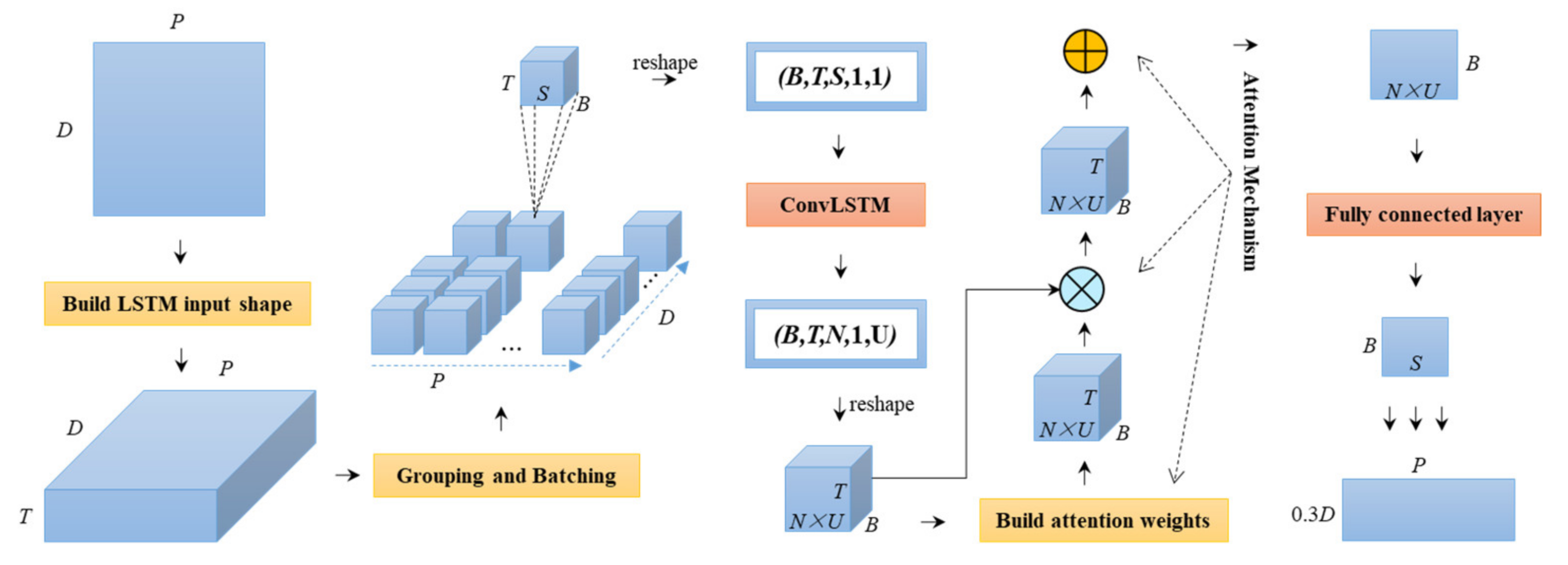
This model includes two parts. The first part builds OC data to match the input shape of ConvLSTM and the second part uses ConvLSTM and a fully connected layer to train and predict OC. The structure of ConvLSTM-F model is shown in Figure 1.
P is the total number of points in selected sea area, D is the total number of days of time series for each point, and the initial input shape is (D, P). For building the input shape for ConvLSTM, the first step is to form input shape for LSTM as (D, T, P), T is time step, and then divide data into small groups in spatial dimension for spatial attention mechanism, and further break data into batches. Now the input data are formed into many cubes with shape (B, T, S). B means batch size and S is group size in spatial dimension.
For the convolutional size, it is S in the spatial dimension and 1 in the time dimension. It means the OC for S points on a day. As there are only OC data, the number of channels is also 1. Taking time step and batch size into account, the input data are reshaped to (B, T, S, 1, 1). If we ignore the channel dimension, for one specified element of B and one specified element of T, the corresponding matrix is (S, 1). The convolutional operation will be applied to this matrix. The convolutional kernel size is (Ks, 1). The kernel size in spatial dimension is Ks and it is 1 in time dimension. After the convolutional operation, the number of output in spatial dimension is calculated by equation below.
N = ( S K s ) / S t r i d e s + 1
where Strides is stride in spatial dimension. The stride in time dimension is also 1. We can also use Equation (1) for the number of output in time dimension. As, in time dimension, the convolutional size is the same as kernel size, its value is 1. So the matrix shape is changed from (S, 1) to (N, 1) after convolution. Taking batch size and time step into account, the shape of output for ConvLSTM becomes (B, T, N, 1, U). U is the number of convolutional filters. Then, we flatten it to (B, T × N × U) and use it as input for the fully connected layer. Now we have the output with shape (B, S) for one batch. As we use 30% data for test, when all batches are completed, the shape of the output for one spatial group will be (0.3D, S). When all spatial groups are completed, the final output for this model is generated with shape (0.3D, P).

2.2. The A-ConvLSTM Model

Attention mechanism in deep learning is the solution used to simulate the attention mechanism of the human brain proposed by Bahdanau et al. [34] and Luong et al. [35]. It can quickly identify the high value information from a large amount of information, strengthen the effect from them, and weaken the effect from the low value information.
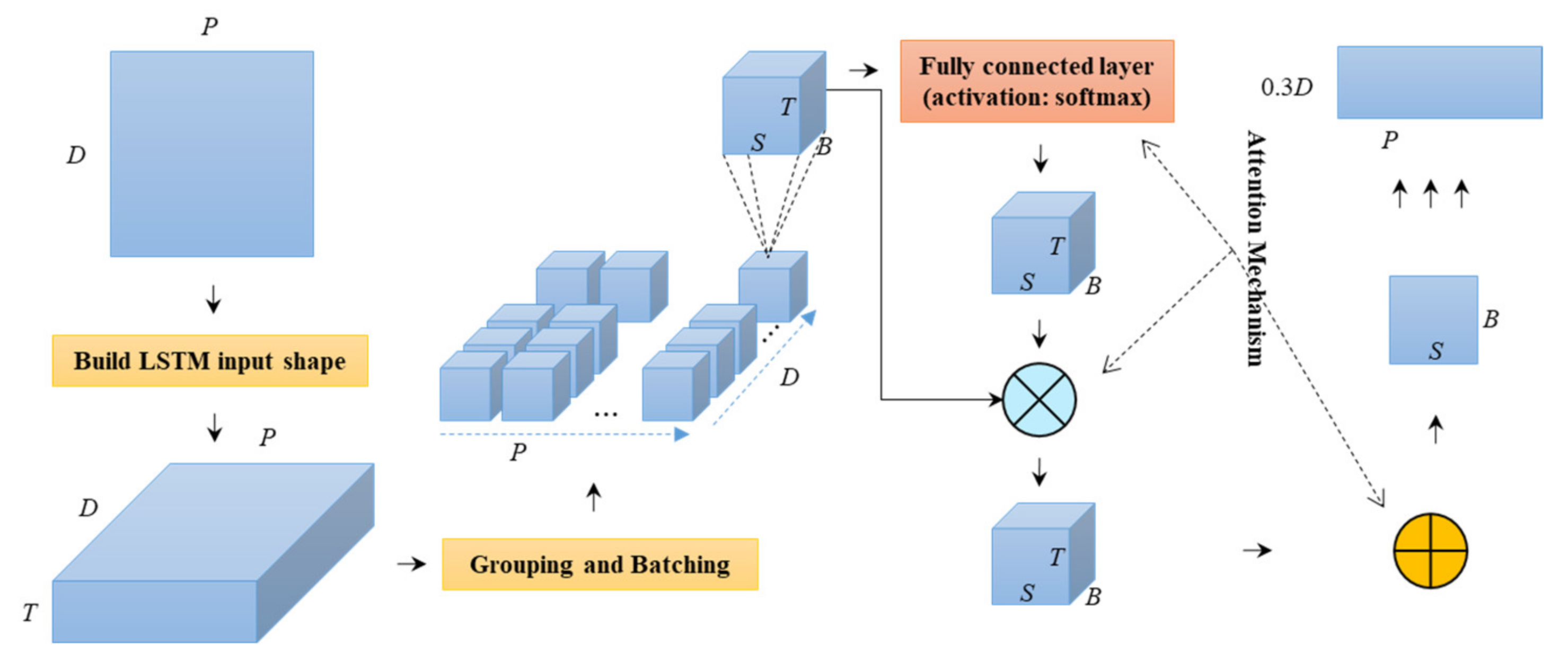
This model will use ConvLSTM to train OC first, and apply attention mechanism to the output of ConvLSTM to strengthen the data with high value information to improve the prediction performance. The structure of A-ConvLSTM is shown in Figure 2.
Until the ConvLSTM generates its output, this model is the same as ConvLSTM-F. Next, this model will reshape the output of ConvLSTM to (B, T, N × U). The attention weight for each element of ConvLSTM output is calculated by equation below.
α b , t , u = exp ( e b , t , u ) i = 0 T 1 exp ( e b , i , u ) ,   0 b < B       0 t < T       0 u < N × U
where B is batch size, T is time step, N is the number of ConvLSTM output in spatial dimension, U stands for the number of convolutional filters, eb,t,u is an element of a cube (reshaped ConvLSTM output), b is the bth day within a batch, t is the tth step of time step T, and u is index of the uth value in the third dimension of (B, T, N × U). The weight tensor will be generated with shape (B, T, N × U) which includes weight for every element of a cube. Next, we will calculate weighted cube by element-wise multiplication between reshaped ConvLSTM output and weight tensor. After this step, the weight context will be calculated through addition in the second dimension of weighted cube; its shape is (B, N × U). Then, we use a fully connected layer to generate output with shape (B, S). Finally, the output of A-ConvLSTM will be generated with shape (0.3D, P) after all spatial groups are completed.

2.3. The P-ATT Model

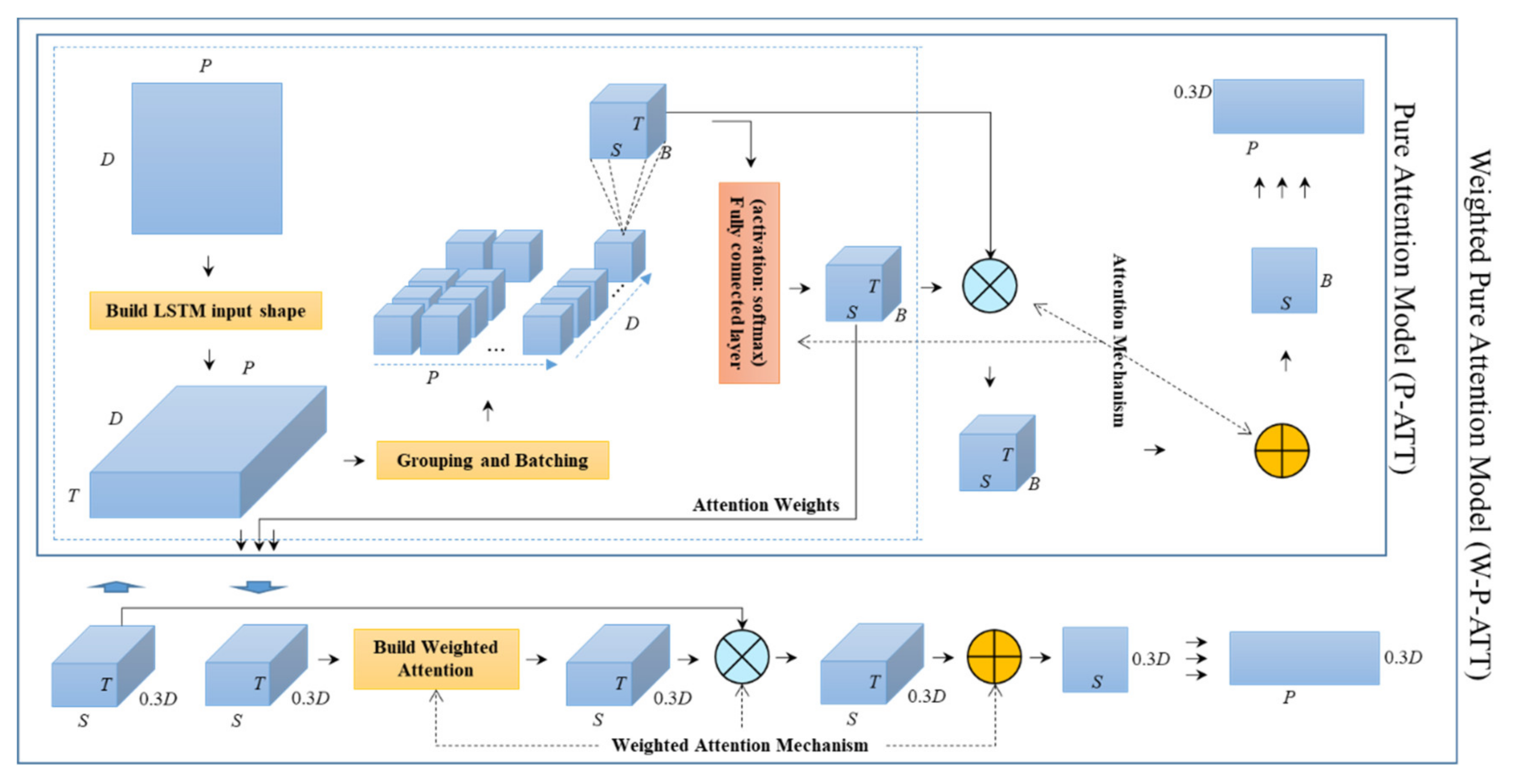
Attention mechanism has been commonly used with deep learning models, such as the above A-ConvLSTM model for OC prediction and the attention-based LSTM model which we used to predict SSH. For researching the power for the pure attention mechanism, Vaswani et al. [42] from the Google machine translation team proposed a Transformer model based on pure attention mechanism for machine translation, which was better than deep learning models plus attention mechanism. So, for OC prediction, we designed the pure attention (P-ATT) model. The structure of P-ATT model is shown in Figure 3.
The data pre-processing part is the same as A-ConvLSTM. It does not use ConvLSTM to train the OC data, but calculates the attention weight for input OC data directly using fully connected layer with softmax as activation function. The equation used to calculate attention weight is also Equation (2). For an input cube with shape (B, T, S), there will be attention weight tensor with the same shape. Next, we will calculate weighted cube by element-wise multiplication between input cube and weight tensor. The weighted cube keeps the same shape as the input cube. The weight context will be calculated through addition in the second dimension of weighted cube and its shape becomes (B, S). It will be used directly as the output of one batch for a spatial group; the output shape will be (B, P) for a spatial group, and the finally output shape will be (0.3D, P) for the selected sea area.

2.4. The W-P-ATT Model

The P-ATT model can fully mine the advantage of the attention mechanism, and let high value information play more critical role for OC prediction. If we strengthen the weight for high value information, the performance should be improved further. So, we proposed the weighted pure attention (W-P-ATT) model based on P-ATT model. The structure of W-P-ATT model is shown in Figure 4.
This model will first use the P-ATT model to train OC. We will have the trained model for OC prediction. After that, we can obtain the attention weight for each element within the input data from the trained model, and the attention weight will be used for W-P-ATT model. For a spatial group, the output weight tensor from P-ATT model has the shape (0.3D, T, S). Here, we will start the procedure to build the weighted attention weight tensor for the output weight tensor.
max _ α = max _ α b , s , 1 = max 0 t < T α b , s , t   0 b < B , 0 s < S                   ( B ,   S ,   1 )
The shape of max_α is (B, S, 1). We will duplicate its 3rd dimension from 1 to T through equation below.
d u p max _ α = max _ α · 1 1 × T                                 ( B ,   S ,   1 ) · ( 1 ,   T ) = ( B ,   S ,   T )
Now, we create a factor tensor and the value of its each element is 0 or 1. It is obtained by element-wise division between α and dupmax α and rounding down the value to 0 or 1. The value will be zero where it is non-maximal attention weight and 1 where it is maximum attention weight. It is calculated by equation below.
0 _ 1 _ f = α d u p max _ α               ( B ,   S ,   T )
Next, we introduce the weight parameter for attention weight. It will take away partial weight from non-maximal attention weight to maximum attention weight. Let the percentage of weight taken away be ω. For 0_1_f, we change 0 to ω and keep 1 unchanged through equation below.
ω _ 1 _ f = 0 _ 1 _ f ×   ( 1 ω ) + ( α α + ω )   ( B ,   S ,   T )
When we have the percentage, for non-maximal attention weight we can calculate its part which will be take away and the maximum attention weight will not change at here. This part can be calculated by element-wise multiplication between ω_1_f and α. Then, we add the part taken away to the maximum attention weight through the addition in the 3rd dimension. These two steps are expressed by equation below.
s u m α = s u m _ α b , s , 1 = t = 0 T 1 ( ω _ 1 _ f b , s , t × α b , s , t )   0 b < B , 0 s < S   ( B ,   S ,   1 )
It is time to calculate the new weight for the maximum attention weight. We will first duplicate the 3rd dimension of sumα from 1 to T, and then obtain the new weight by element-wise multiplication between duplicated sumα and 0_1_f. The equation is expressed as below.
w e i g h t e d _ max = 0 _ 1 _ f × ( s u m α · 1 1 × T )   ( B ,   S ,   T )
For the non-maximal attention weight, the part not taken away will be the new weight. It is calculated by the equation below.
w e i g h t e d _ n o n _ max = ( 1 ω _ 1 _ f )   × α   ( B ,   S ,   T )
Now, we can have the entire new weight for an input cube by adding up the new weight of maximum attention weight and the new weight of non-maximal attention weight. The equation is expressed as below.
α = w e i g h t e d _ max + w e i g h t e d _ n o n _ max   ( B ,   S ,   T )
The shape of the new weight tensor for an input cube is (B, S, T), and we will reshape it back to (B, T, S). After merging all batches, it obtains the weighted attention weight for a spatial group with shape (0.3D, T, S). The remaining steps are the same as the P-ATT model, and finally we will have the prediction output with shape (0.3D, P).
For weight parameter ω, the range will be [0, 1). The bigger value will take away more weight from non-maximal attention weight to maximum attention weight and the performance should be better. In the experiment section, we will try different values to show how it affects attention mechanism differently.

3. Experiment

The experiments in this paper predicted OCs using different five models. The first model is CNN-GRU proposed by Thongniran et al. [33]. The second model is ConvLSTM-F which predicts OCs with ConvLSTM plus fully connected layer. The third one is A-ConvLSTM to reflect the effect of attention mechanism to ConvLSTM-F. The fourth model is the pure attention model, P-ATT. The last one is the proposed weighted pure attention model, W-P-ATT. If it is not explicitly defined, the default value of weight parameter ω will be 0.7.

3.1. Data Sets

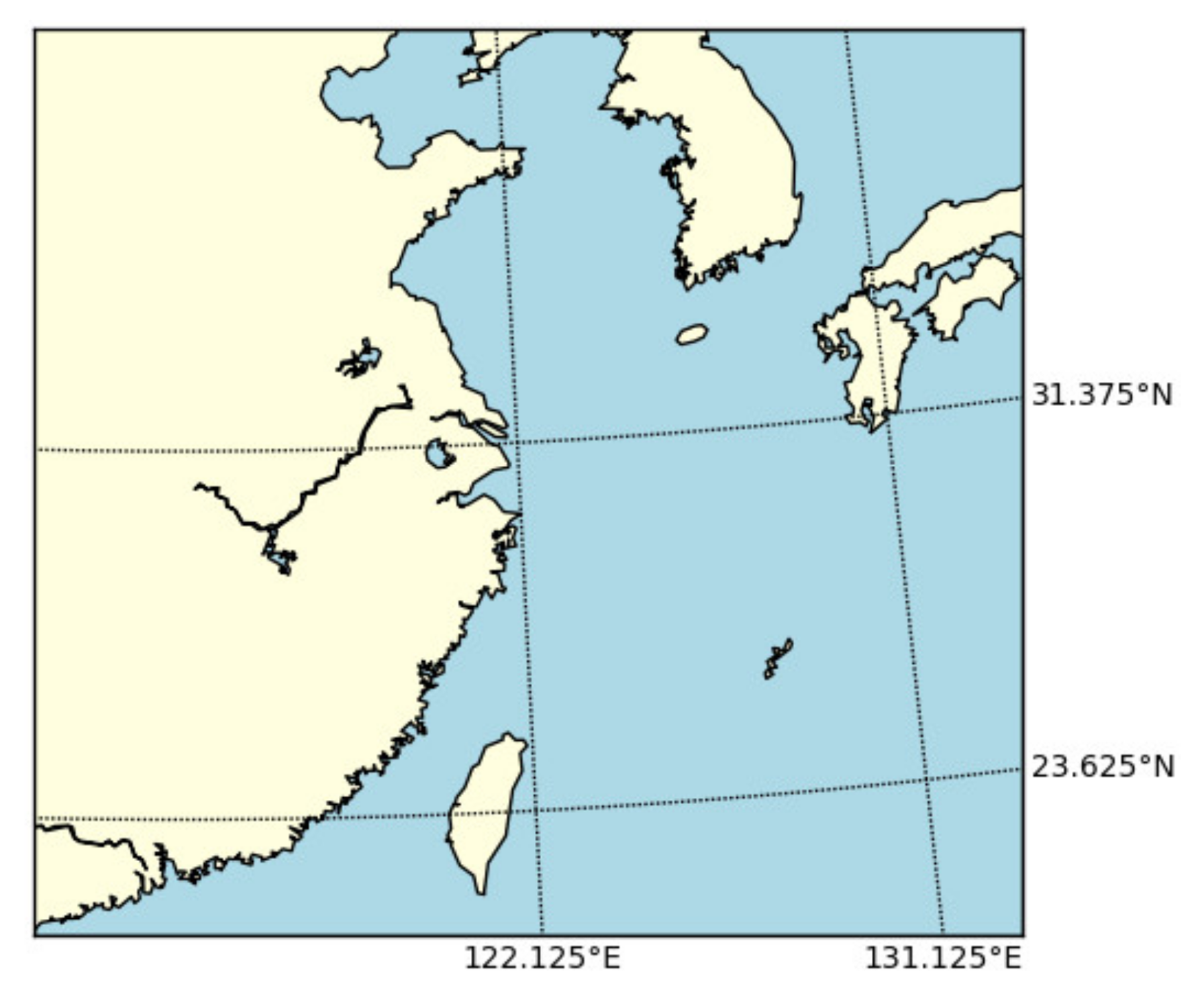
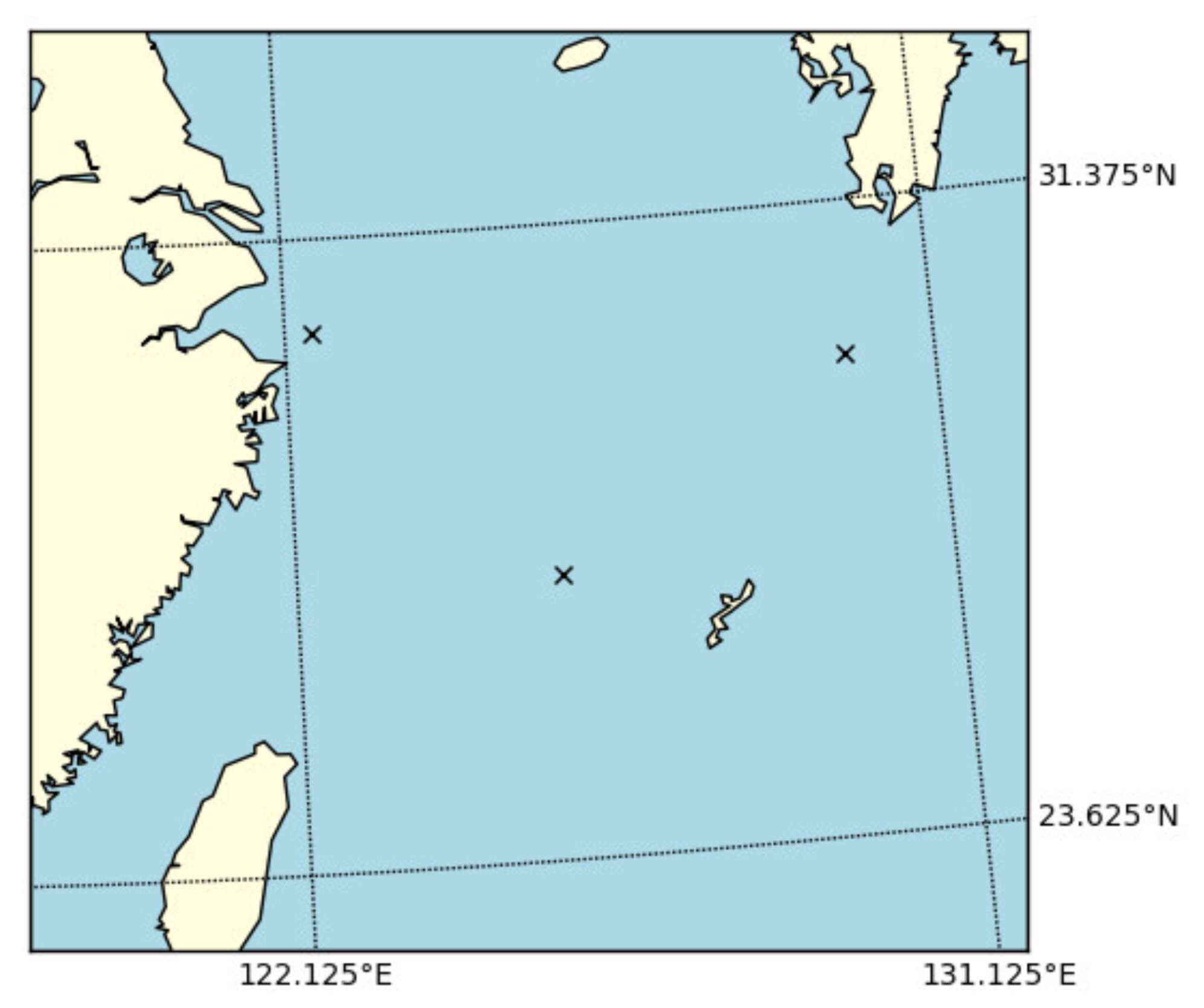
The data sets used in this paper are from the East China Sea, which are China Ocean ReAnalysis (CORA) data from the National Marine Information Center. This data are constructed by combining observations from satellite remote sensing and other platforms. We select OCs for which the depth is ten meters below the surface of the sea. It includes the north component of velocity (u_current) and the east component of velocity (v_current). The spatial resolution is 0.125° × 0.125° and the time resolution is day. The spatial scope for the East China Sea is 23.625° N−31.375° N and 122.125° E−131.125° E (see Figure 5), and we select 2010 points in total in experiments. It includes a total of 3287 days from 1 January 2011 to 14 December 2017.

3.2. Setups

The experiments used the mean absolute error (MAE), root mean square error (RMSE), and correlation coefficient (r) to evaluate the performance of OC prediction for the five different models. Their equations are defined as below:
RMSE = i = 1 n y i x i 2 n
MAE = 1 n i = 1 n | y i x i |
r = i = 1 n x i x ¯ y i y ¯ i = 1 n x i x ¯ 2 i = 1 n y i y ¯ 2
where xi is the actual observed value of time i, yi is the predicted value at the same time, n is the amount of data, x ¯ is the average value of the actual observed values, and y ¯ is the average value of the predicted values.
In order to select optimal key parameters of models, we used hyperband algorithm to identify the parameter values for better performance. For optimizer, we used Adam. For loss function, we used mean square error (mse). The default learning rate of Adam was used and its value was 0.001. The training iterations were defined as 1000 and early stopping was also used for models with patience 10. For data separation, 70% of data were used for training and 30% of data were used for testing. The more detailed information of key parameters is shown in Table 1.

3.3. Results

In this section, we will verify the advantage of the attention mechanism, compare the performance between deep learning model plus attention mechanism and pure attention mechanism, and further show the effect of weighed attention mechanism for improving prediction performance.

3.3.1. Performance Comparison for Spatial Points

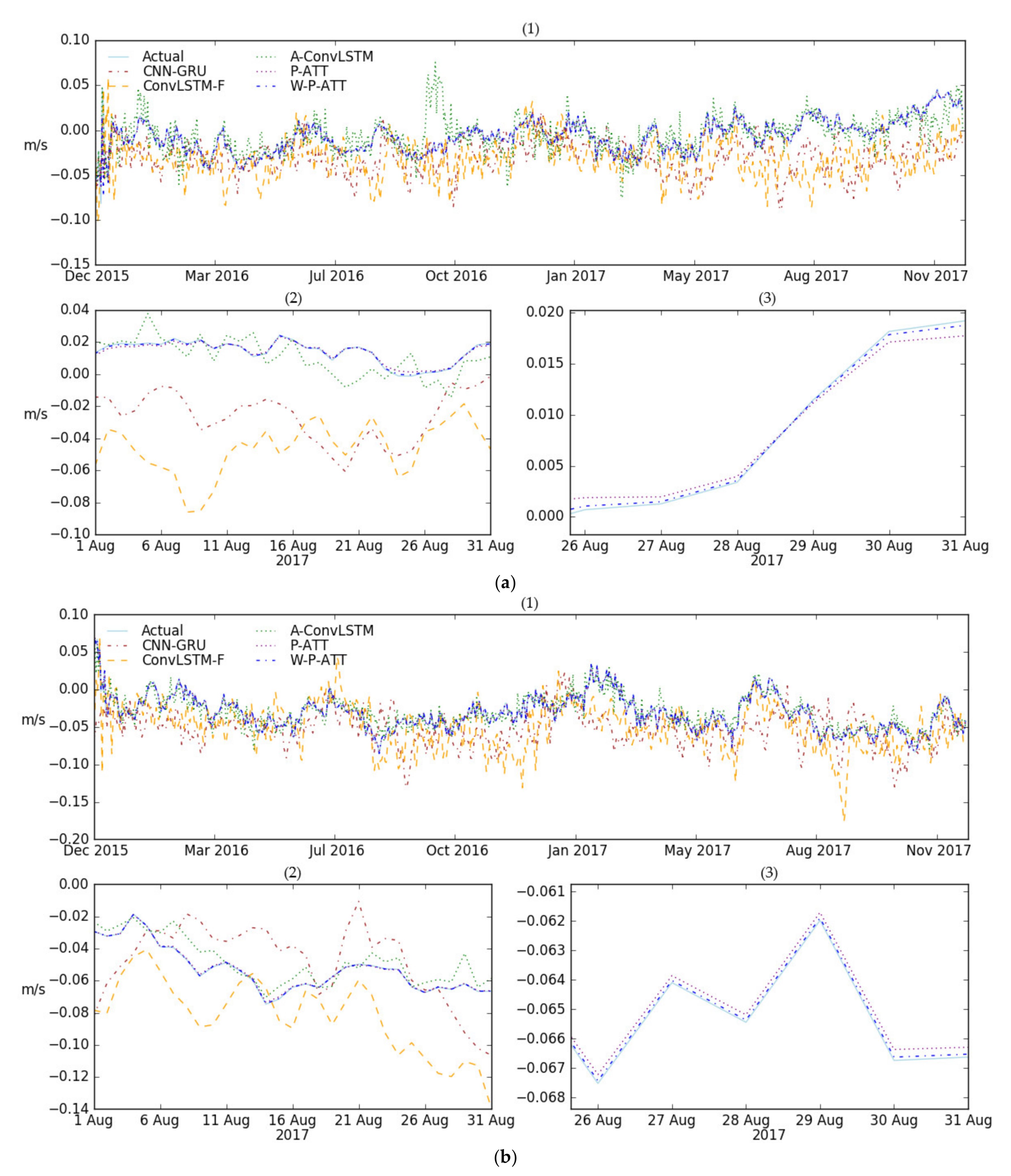
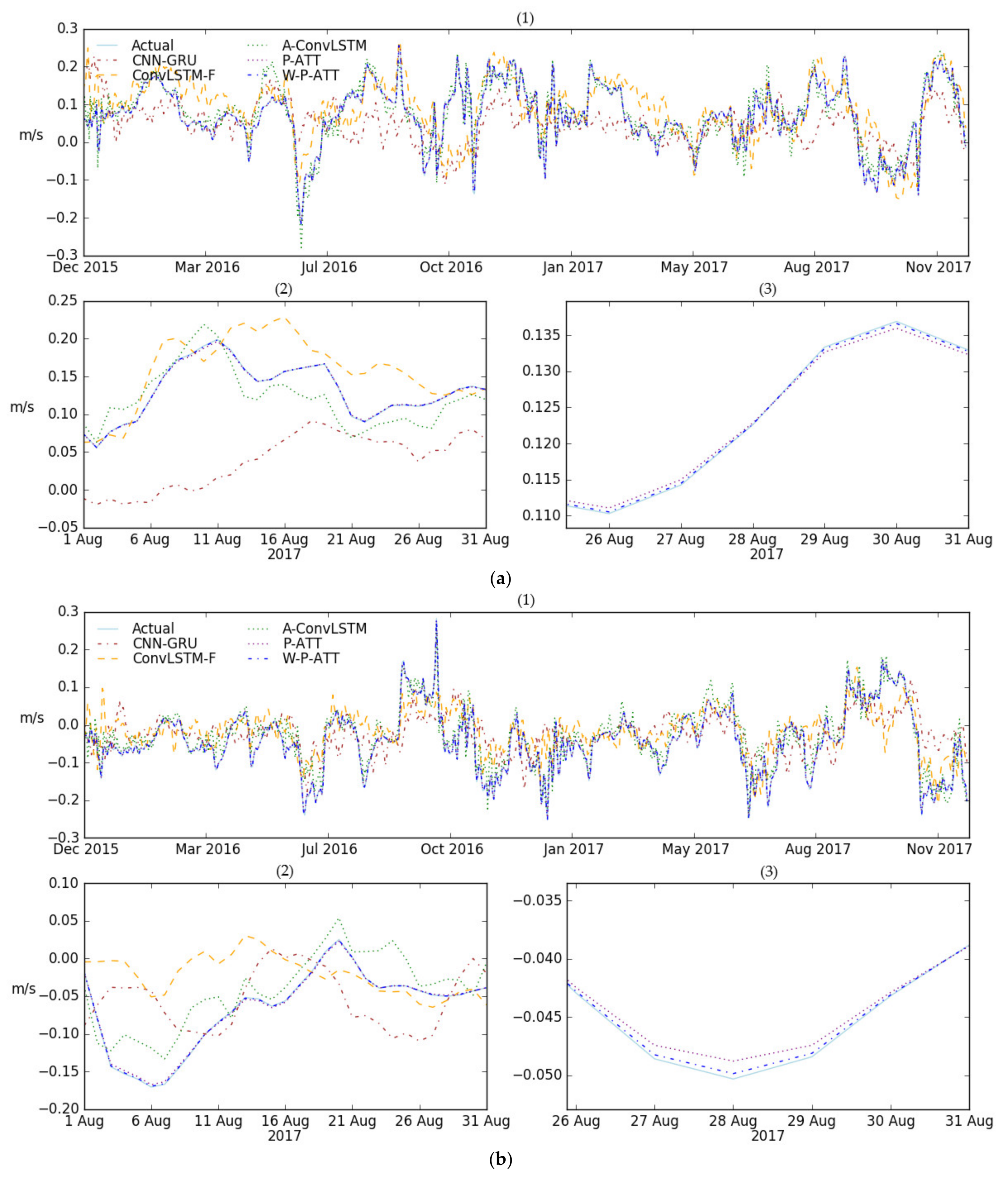
The easiest way to compare the performance of different models is to select some spatial points and show their OC trends in time dimension. We evenly selected three points in the selected sea area as shown in Figure 6. These three spatial points are (122.5° E, 30.25° N), (129.875° E, 29.5° N), and (125.75° E, 27.125° N).
We compared the predicted OCs with the observed OCs for these three points. The comparison results are shown in Figure 7, Figure 8 and Figure 9. There are two figures for each point; the first is for u_current, and the second is for v_current.
For the following three figures, we separate each figure to three subfigures. The subfigure (1) is the OC trend comparison for the entire time range. In order to more clearly reflect the performance difference between the five models, we select one month to show the comparison results. The subfigure (2) is the comparison result for August 2017. It is also difficult to see the difference between P-ATT and W-P-ATT in subfigure (2), so we use a shorter period in August 2017 to compare the performance between these two models in subfigure (3).
It is clear to see from Figure 7, Figure 8 and Figure 9 that ConvLSTM-F is similar to CNN-GRU. Both have big differences with actual values. After applying attention mechanism, A-ConvLSTM greatly improves the prediction performance and is much better than ConvLSTM-F. The P-ATT further improves the performance and is very close to the actual values after switching to the pure attention mechanism. Based on P-ATT, we introduce weighted pure attention mechanism. As we can see from these three figures, the W-P-ATT is the best one and consistent with the actual values. It proves that the pure attention mechanism can better take advantage of the key elements with high value information for target value than the combination of deep learning models and the attention mechanism, and the weighted pure attention mechanism further refines the pure attention mechanism by introducing the weight parameter and can better identify the importance of the key elements.
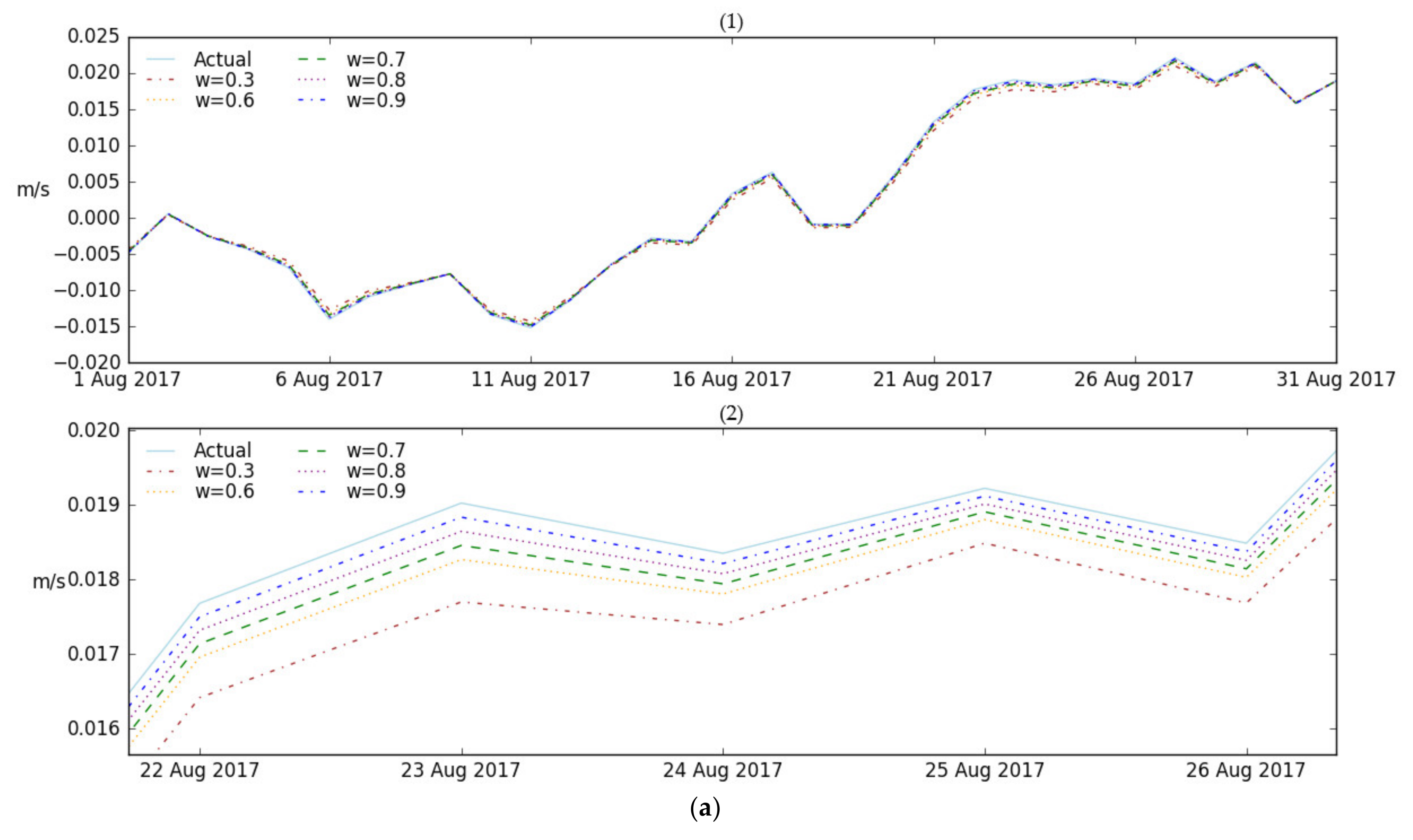
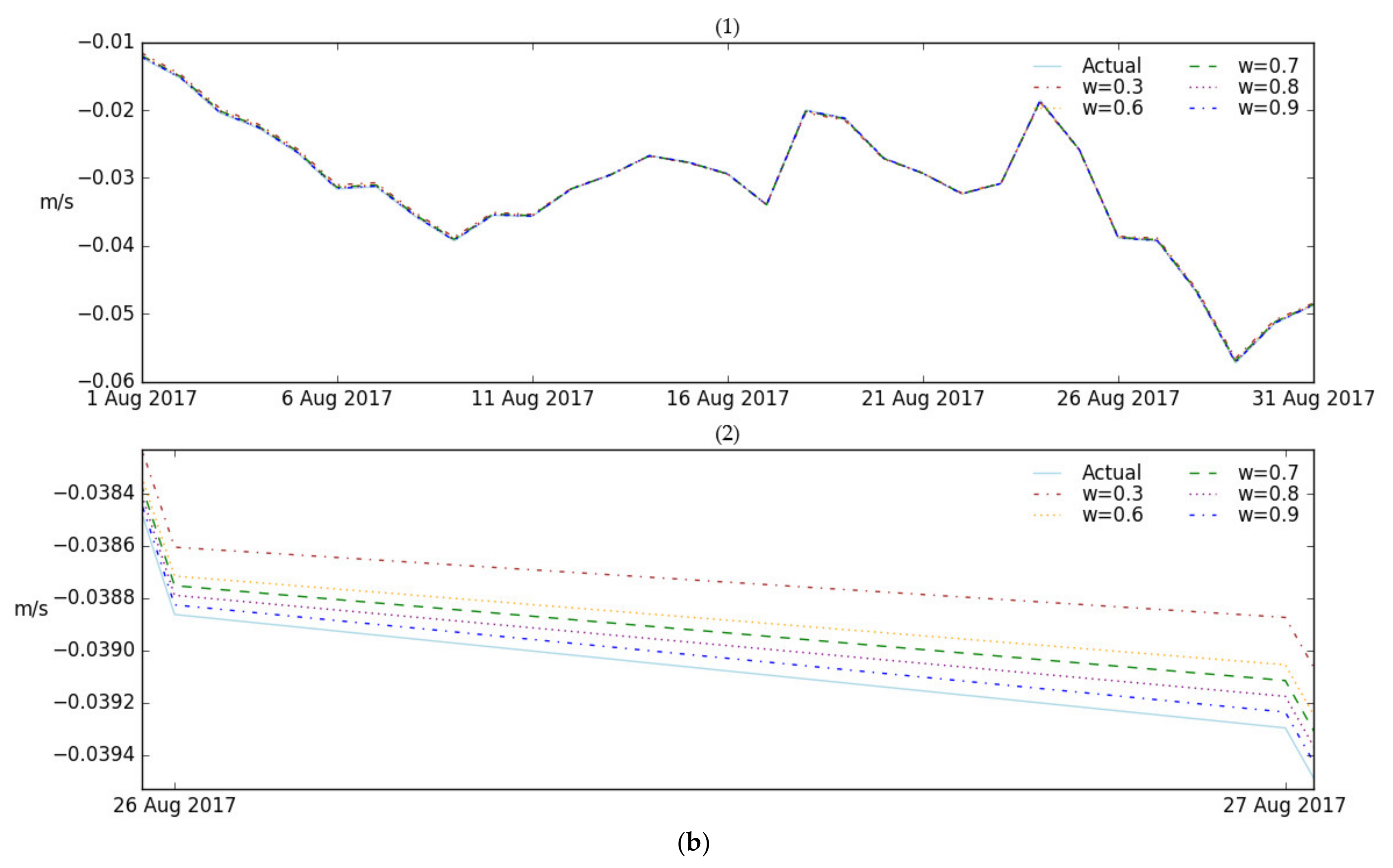
For the W-P-ATT model, the performance will be different if we set a different value for ω. As stated in Section 2.4, generally the bigger value will have better performance. For spatial point (129.875° E, 29.5° N), we used five different ω for W-P-ATT model and compared the predicted OCs with the observed OCs for them. The comparison results are shown in Figure 10.
As we can see from Figure 10, for both of u_current and v_current, the performance is worst when the value of weight parameter ω is 0.3. When we set the value of ω from 0.6 to 0.9, the performances are close to each other and much better than the performance when weight value is 0.3. The performance become better and better along with the increment of ω from 0.6 to 0.9. Therefore, the performance change is consistent with the change of the weight parameter value. It proved that the performance improves with bigger ω.

3.3.2. Performance Comparison through MAE and RMSE

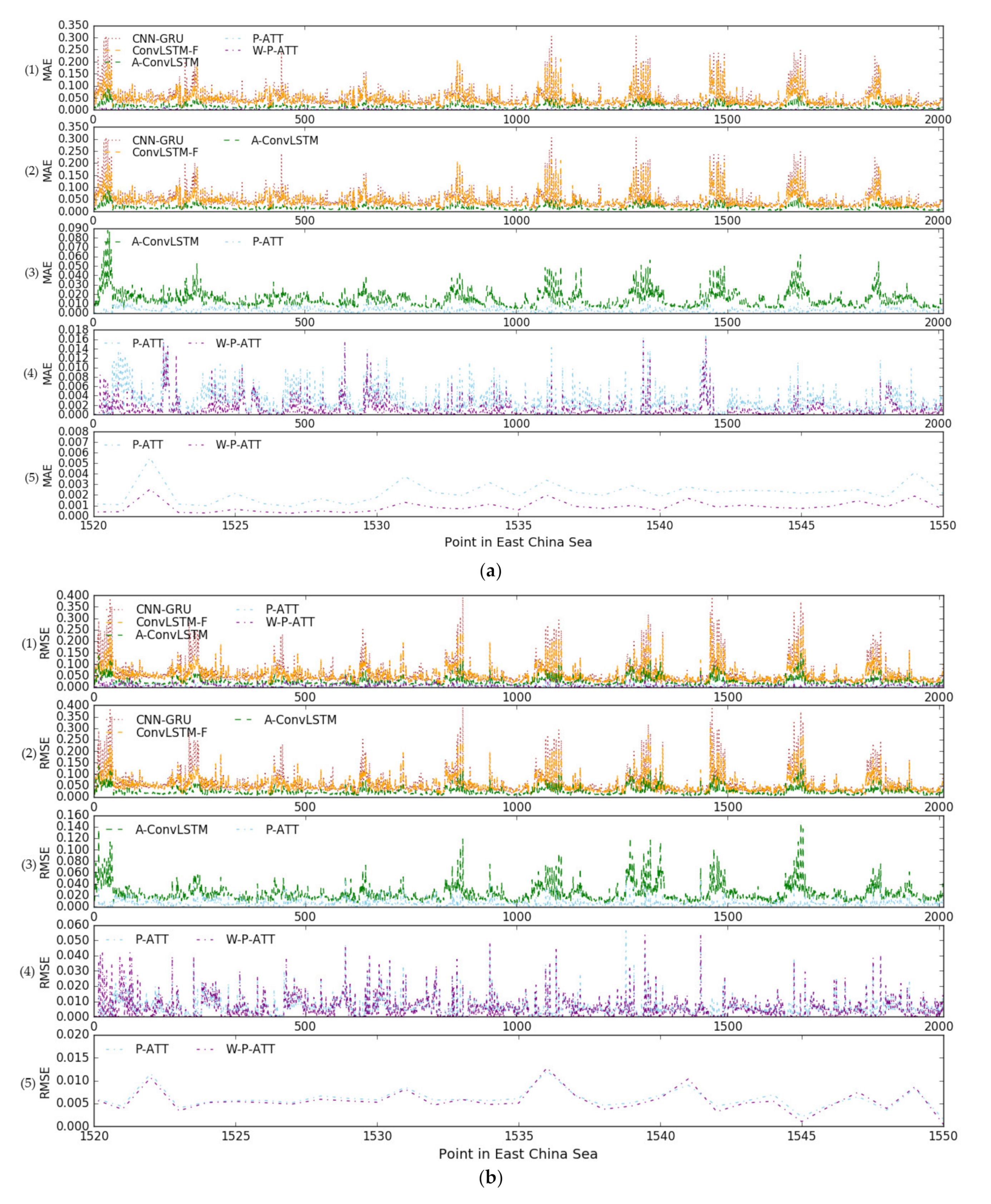
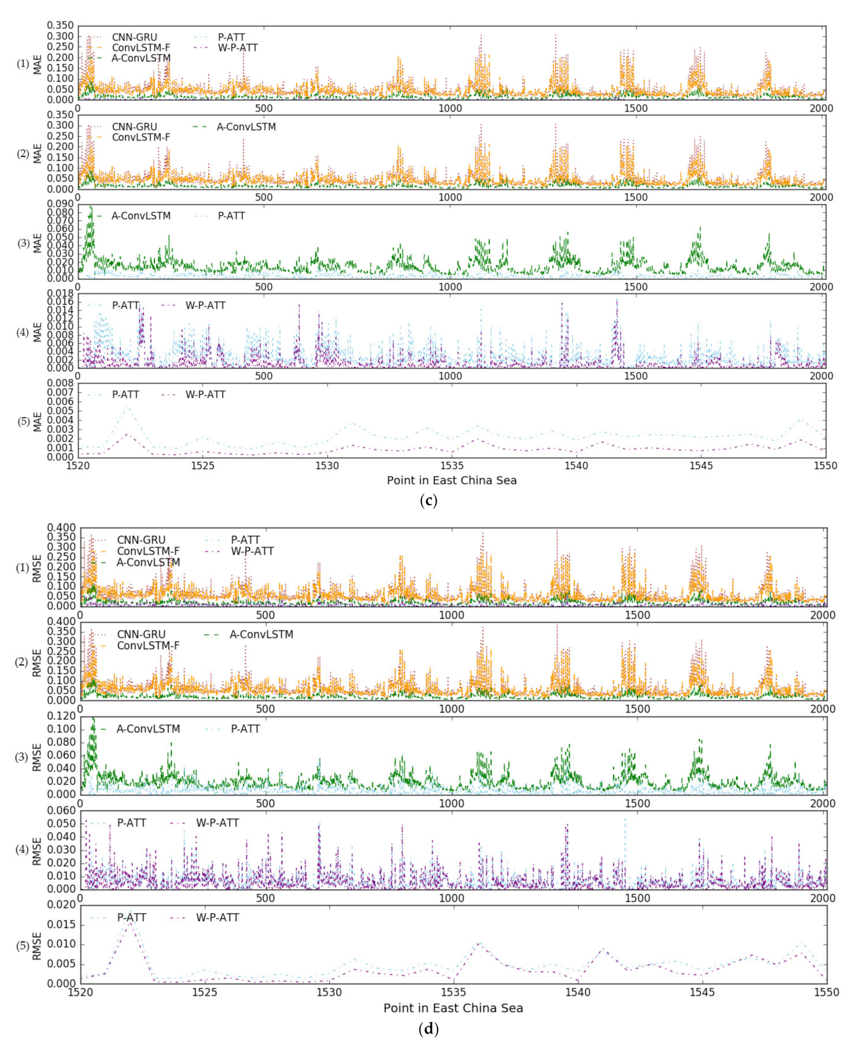
In this section, we will compare MAE and RMSE between different models to further verify the advantage of the proposed model. The MAE and RMSE can be calculated by Equations (11) and (12), and the comparison results are shown in Figure 11.
It is clear to see from Figure 11 that CNN-GRU and ConvLSTM-F have the similar MAE and RMSE. The A-ConvLSTM has much better MAE and RMSE after attention mechanism adoption. The pure attention mechanism model, P-ATT, further improves the prediction performance. After introducing weight adjustment for the pure attention mechanism model, the weighted pure attention model, W-P-ATT, becomes the best model from the MAE and RMSE perspective. In order to see the comparison results between P-ATT and W-P-ATT more clearly, we use subfigure (5) to show the differences through a short point range from point 1520 to point 1550. From subfigure (5), for both u_current and v_current, it clearly shows the advantage of the proposed model.

3.3.3. Performance Comparison through Distribution of MAE and RMSE

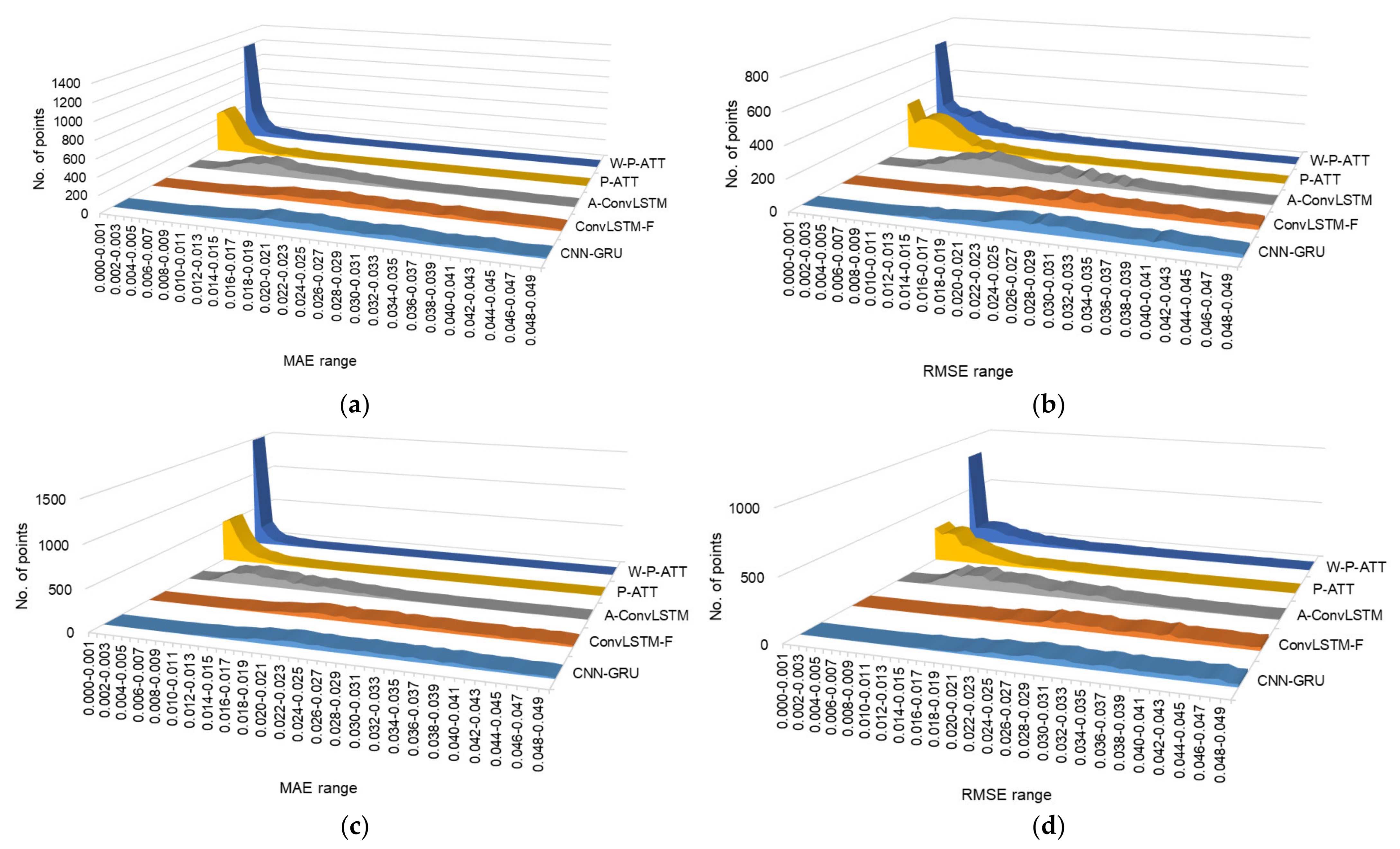
In this section, we will use distribution of MAE and RMSE to further validate the performance of the proposed model. The distribution can clearly show the performance differences between the five models in another dimension. Figure 12 shows the MAE and RMSE distributions for every models.
As we can see from Figure 12, for both of MAE and RMSE, the most points for CNN-GRU and ConvLSTM-F are distributed between 0.02 and 0.04, and the main distribution for A-ConvLSTM shifts left and is between 0.003 and 0.018. The P-ATT model shifts left a lot further than A-ConvLSTM and is mainly distributed between 0 and 0.007. The proposed model, W-P-ATT, is much better than P-ATT and moves most of points to the very left area. It proves the W-P-ATT is the best model in the perspective of MAE/RMSE distribution.
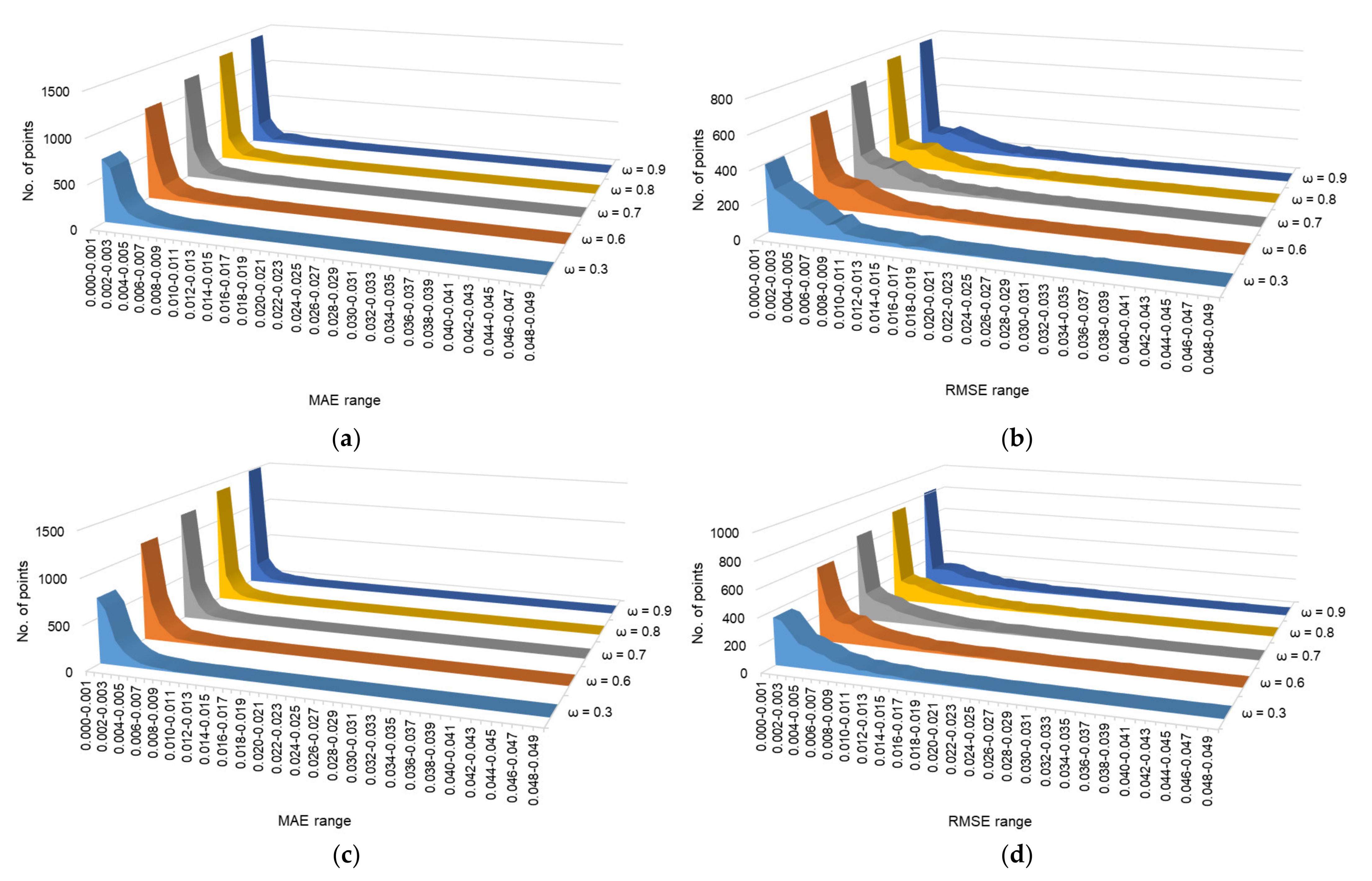
In Section 3.3.1, we verified the W-P-ATT model with different values of ω and found that the performance became better with a bigger ω. Next, we will use MAE and RMSE to further verify this. We will use the five different ω for the W-P-ATT model to compare their MAE and RMSE distributions. The comparison results are shown in Figure 13.
It is clear to see from Figure 13 that as ω grows the MAE and RMSE distribution improves. Therefore, it further proves that the performance of OC prediction becomes better with a bigger ω.

3.3.4. Performance Comparison through the Average MAE, RMSE, and r

In the above sections, we graphically verified the advantages of the proposed model in different dimensions. In this section, we will use the average MAE, RMSE, and r to further show the performance difference for different models. The comparison results are shown in Table 2.
As we can see from the table, the proposed model has the best average MAE/RMSE/r for both u_current and v_current. The MAE of the proposed model decreases by 90% for both of u_current and v_current compared to A-ConvLSTM, and 65% for u_current and 86% for v_current compared to P-ATT. The RMSE of the proposed model decreases by more than 75% for both of u_current and v_current compared to A-ConvLSTM, and more than 20% for both u_current and v_current compared to P-ATT. The proposed model also has a much better r than A-ConvLSTM and P-ATT. The r reaches up to more than 0.99 for both u_current and v_current. It proves that the proposed model significantly improves the performance of OC prediction.

4. Discussion

As stated in Section 3, we set up five models in order to show the advantages of the proposed model. The first model was CNN-GRU proposed by Thongniran et al. [33]. It can analyze the OC in both of spatial and time dimensions for improving the performance of OC prediction. The ConvLSTM has the same features as CNN-GRU, so we used it as the second model. As we can see from the experiments, they had a similar prediction performance and the performance was not good. Based on the ConvLSTM, the third model, A-ConvLSTM, integrated the attention mechanism to the second model. The attention mechanism can make the ConvLSTM to focus more on the high value elements for predicting the target elements, so the performance should be better than only ConvLSTM. The experiments proved this hypothesis. However, the prediction performance was still not good enough, so we supposed that the integration between the ConvLSTM and attention mechanism did not identify the importance of the key elements enough comparing to the pure attention mechanism. We introduced the fourth model, P-ATT, which used the pure attention mechanism for OC prediction. The experiments verified our assumption that the P-ATT significantly improved the predict performance comparing to A-ConvLSTM. As the P-ATT could better identify the key elements for better performance, we had a further assumption that the performance would be further improved if we adjusted the attention weights to let the most key elements have more attention weights. So, based on P-ATT, we designed the fifth model, the proposed model in this paper, W-ATT, by introducing the weight parameter to move attention weights to the most key elements from other elements. According to the experiment results, this assumption was also proven, and it greatly improved the performance than the pure attention mechanism.
In the experiments, we selected 2010 points in spatial dimension and 3287 days for each point in time dimension from the East China Sea. The results showed that the proposed model was most consistent with the observed OC, had the most stable and lowest MAE/RMSE, had the best r, and also had the best distribution of MAE and RMSE. So the experiments proved that the proposed model was reliable for OC prediction with high performance for a wide time range and large spatial scope.

5. Conclusions

In this paper, we analyzed the bottleneck of OC prediction performance caused by not adequately identifying the importance of the key elements and not fully taking advantage of the most significant elements with the attention mechanism, and proposed an innovative deep learning model based on weighted pure attention mechanism (W-P-ATT) for OC prediction. The proposed model can resolve these problems for OC prediction through the pure attention mechanism and the optimization for the pure attention mechanism via the weight parameter. This was achieved by leveraging the pure attention mechanism, introducing the weight parameter for attention weight, and adjusting the attention weight to make the key elements play more critical roles for OC prediction. The proposed model demonstrates reliable results, the MAE is 0.0017 m/s for u_current and 0.0014 m/s for v_current, the RMSE is 0.0051 m/s for u_current and 0.0049 m/s for v_current, and the correlation coefficient reaches up to 0.99. The experiment results revealed that the proposed model could break through the bottleneck and significantly improve the performance for OC prediction.

Author Contributions

Conceptualization, J.L. and J.Y.; methodology, J.L.; software, K.L.; validation, J.L., J.Y. and L.X.; formal analysis, J.L.; investigation, J.L.; resources, J.L.; data curation, K.L.; writing—original draft preparation, J.L.; writing—review and editing, J.Y., K.L and L.X.; visualization, J.L.; supervision, J.Y.; project administration, L.X.; and funding acquisition, J.L. and L.X. All authors have read and agreed to the published version of the manuscript.

Funding

This paper was funded by the National Key R&D Program of China (2016YFC1401900), the Key Laboratory of Digital Ocean, SOA, of China (B201801030), and the Science and Technology Department of Zhejiang Province (LGG21F020008).

Institutional Review Board Statement

Not applicable.

Informed Consent Statement

Not applicable.

Data Availability Statement

The data that support the findings of this study are openly available from CORAv2.0 in the China National Marine Data Center at http://mds.nmdis.org.cn/pages/dataView.html?type=2&id=a5da2a0528904471b3a326c3cc85997d (accessed on 13 April 2022), and the reference year from 2011 to 2017.

Acknowledgments

We appreciate the National Marine Information Center for the CORA data.

Conflicts of Interest

The authors declare no conflict of interest.

References

  1. Klemas, V. Remote sensing of coastal and ocean currents: An overview. J. Coast. Res. 2012, 28, 576–586. [Google Scholar] [CrossRef]
  2. Armour, K.C.; Marshall, J.; Scott, J.R.; Donohoe, A.; Newsom, E.R. Southern Ocean warming delayed by circumpolar upwelling and equatorward transport. Nat. Geosci. 2016, 9, 549–554. [Google Scholar] [CrossRef]
  3. Dambach, J.; Raupach, M.J.; Leese, F.; Schwarzer, J.; Engler, J.O. Ocean currents determine functional connectivity in an Antarctic deep-sea shrimp. Mar. Ecol. 2016, 37, 1336–1344. [Google Scholar] [CrossRef]
  4. Iwasaki, S.; Isobe, A.; Kako, S.I.; Uchida, K.; Tokai, T. Fate of microplastics and mesoplastics carried by surface currents and wind waves: A numerical model approach in the Sea of Japan. Mar. Pollut. Bull. 2017, 121, 85–96. [Google Scholar] [CrossRef] [PubMed]
  5. Zhang, W.; Zhang, S.; Wang, J.; Wang, Y.; Mu, J.; Wang, P.; Lin, X.; Ma, D. Microplastic pollution in the surface waters of the Bohai Sea. Environ. Pollut. 2017, 231, 541–548. [Google Scholar] [CrossRef] [PubMed]
  6. Tamtare, T.; Dumont, D.; Chavanne, C. Extrapolating Eulerian ocean currents for improving surface drift forecasts. J. Oper. Oceanogr. 2021, 14, 71–85. [Google Scholar] [CrossRef]
  7. Kane, I.A.; Clare, M.A.; Miramontes, E.; Wogelius, R.; Rothwell, J.J.; Garreau, P.; Pohl, F. Seafloor microplastic hotspots controlled by deep-sea circulation. Science 2020, 368, 1140–1145. [Google Scholar] [CrossRef]
  8. Courtene-Jones, W.; Quinn, B.; Gary, S.F.; Mogg, A.O.; Narayanaswamy, B.E. Microplastic pollution identified in deep-sea water and ingested by benthic invertebrates in the Rockall Trough. North Atlantic Ocean. Environ. Pollut. 2017, 231, 271–280. [Google Scholar] [CrossRef] [Green Version]
  9. Pohl, F.; Eggenhuisen, J.T.; Kane, I.A.; Clare, M.A. Transport and burial of microplastics in deep-marine sediments by turbidity currents. Environ. Sci. Technol. 2020, 54, 4180–4189. [Google Scholar] [CrossRef]
  10. Nooteboom, P.D.; Bijl, P.K.; van Sebille, E.; Von Der Heydt, A.S.; Dijkstra, H.A. Transport bias by ocean currents in sedimentary microplankton assemblages: Implications for paleoceanographic reconstructions. Paleoceanogr. Paleocl. 2019, 34, 1178–1194. [Google Scholar] [CrossRef]
  11. Yamada, M.; Zheng, J. 240Pu/239Pu atom ratios in water columns from the North Pacific Ocean and Bering Sea: Transport of Pacific Proving Grounds-derived Pu by ocean currents. Sci. Total Environ. 2020, 718, 137362. [Google Scholar] [CrossRef] [PubMed]
  12. Singh, Y.; Sharma, S.; Sutton, R.; Hatton, D.; Khan, A. A constrained A* approach towards optimal path planning for an unmanned surface vehicle in a maritime environment containing dynamic obstacles and ocean currents. Ocean Eng. 2018, 169, 187–201. [Google Scholar] [CrossRef] [Green Version]
  13. Shen, Y.T.; Lai, J.W.; Leu, L.G.; Lu, Y.C.; Chen, J.M.; Shao, H.J.; Chen, H.W.; Chang, K.T.; Terng, C.T.; Chang, Y.C.; et al. Applications of ocean currents data from high-frequency radars and current profilers to search and rescue missions around Taiwan. J. Oper. Oceanogr. 2019, 12, S126–S136. [Google Scholar] [CrossRef] [Green Version]
  14. Wen, J.; Yang, J.; Wang, T. Path Planning for Autonomous Underwater Vehicles under the Influence of Ocean Currents Based on a Fusion Heuristic Algorithm. IEEE Trans. Veh. Technol. 2021, 70, 8529–8544. [Google Scholar] [CrossRef]
  15. Immas, A.; Do, N.; Alam, M.R. Real-time in situ prediction of ocean currents. Ocean Eng. 2021, 228, 108922. [Google Scholar] [CrossRef]
  16. Grossi, M.D.; Kubat, M.; Özgökmen, T.M. Predicting particle trajectories in oceanic flows using artificial neural networks. Ocean Model. 2020, 156, 101707. [Google Scholar] [CrossRef]
  17. Peng, Z.; Wang, J.; Wang, J. Constrained control of autonomous underwater vehicles based on command optimization and disturbance estimation. IEEE Trans. Ind. Electron. 2018, 66, 3627–3635. [Google Scholar] [CrossRef]
  18. Elhaki, O.; Shojaei, K. Neural network-based target tracking control of underactuated autonomous underwater vehicles with a prescribed performance. Ocean Eng. 2018, 167, 239–256. [Google Scholar] [CrossRef]
  19. Fossen, T.I.; Lekkas, A.M. Direct and indirect adaptive integral line-of-sight path-following controllers for marine craft exposed to ocean currents. Int. J. Adapt. Control Signal Process. 2017, 31, 445–463. [Google Scholar] [CrossRef]
  20. Vu, M.T.; Le Thanh, H.N.N.; Huynh, T.T.; Thang, Q.; Duc, T.; Hoang, Q.D.; Le, T.H. Station-keeping control of a hovering over-actuated autonomous underwater vehicle under ocean current effects and model uncertainties in horizontal plane. IEEE Access 2021, 9, 6855–6867. [Google Scholar] [CrossRef]
  21. Sarkar, D.; Osborne, M.A.; Adcock, T.A. Spatiotemporal prediction of tidal currents using Gaussian processes. J. Geophys. Res. Ocean. 2019, 124, 2697–2715. [Google Scholar] [CrossRef]
  22. Yang, G.; Wang, H.; Qian, H.; Fang, J. Tidal current short-term prediction based on support vector regression. In Proceedings of the 2nd Asia Conference on Power and Electrical Engineering (ACPEE), Shanghai, China, 24–26 March 2017. [Google Scholar]
  23. Kavousi-Fard, A.; Su, W. A combined prognostic model based on machine learning for tidal current prediction. IEEE Geosci. Remote Sens. Lett. 2017, 55, 3108–3114. [Google Scholar] [CrossRef]
  24. Remya, P.; Kumar, R.; Basu, S. Forecasting tidal currents from tidal levels using genetic algorithm. Ocean Eng. 2012, 40, 62–68. [Google Scholar] [CrossRef]
  25. Dauji, S.; Deo, M.C.; Bhargava, K. Prediction of ocean currents with artificial neural networks. ISH J. Hydraul. Eng. 2015, 21, 14–27. [Google Scholar] [CrossRef]
  26. Bayindir, C. Predicting the Ocean Currents Using Deep Learning, version 1.0. arXiv 2019, arXiv:1906.08066. [Google Scholar]
  27. Dauji, S.; Deo, M.C. Improving numerical current prediction with Model Tree. Indian J. Geo-Mar. Sci. 2020, 49, 1350–1358. Available online: http://nopr.niscair.res.in/handle/123456789/55314 (accessed on 8 December 2021).
  28. Sarkar, D.; Osborne, M.A.; Adcock, T.A. Prediction of tidal currents using bayesian machine learning. Ocean Eng. 2018, 158, 221–231. [Google Scholar] [CrossRef]
  29. Saha, D.; Deo, M.C.; Joseph, S.; Bhargava, K. A combined numerical and neural technique for short term prediction of ocean currents in the Indian Ocean. Environ. Syst. Res. 2016, 5, 4. [Google Scholar] [CrossRef] [Green Version]
  30. Jirakittayakorn, A.; Kormongkolkul, T.; Vateekul, P.; Jitkajornwanich, K.; Lawawirojwong, S. Temporal kNN for short-term ocean current prediction based on HF radar observations. In Proceedings of the 2017 14th International Joint Conference on Computer Science and Software Engineering (JCSSE), Nakhon Si Thammarat, Thailand, 12–14 July 2017. [Google Scholar] [CrossRef]
  31. Ren, L.; Hu, Z.; Hartnett, M. Short-Term forecasting of coastal surface currents using high frequency radar data and artificial neural networks. Remote Sens. 2018, 10, 850. [Google Scholar] [CrossRef] [Green Version]
  32. Zhang, Z.; Hou, M.; Zhang, F.; Edwards, C.R. An LSTM based Kalman filter for spatio-temporal ocean currents assimilation. In Proceedings of the 14th International Conference on Underwater Networks & Systems, Atlanta, GA, USA, 23–25 October 2019. [Google Scholar] [CrossRef]
  33. Thongniran, N.; Vateekul, P.; Jitkajornwanich, K.; Lawawirojwong, S.; Srestasathiern, P. Spatio-temporal deep learning for ocean current prediction based on HF radar data. In Proceedings of the 16th International Joint Conference on Computer Science and Software Engineering (JCSSE), Pattaya, Thailand, 10–12 July 2019. [Google Scholar] [CrossRef]
  34. Bahdanau, D.; Cho, K.; Bengio, Y. Neural machine translation by jointly learning to align and translate version 7.0. arXiv 2016, arXiv:1409.0473. [Google Scholar]
  35. Luong, M.T.; Pham, H.; Manning, C.D. Effective approaches to attention-based neural machine translation version 5.0. arXiv 2015, arXiv:1508.04025. [Google Scholar]
  36. Chen, P.; Chi, M.Y. STAGRU: Ocean Surface Current Spatio-Temporal Prediction Based on Deep Learning. In Proceedings of the 2021 International Conference on Computer Information Science and Artificial Intelligence (CISAI), Kunming, China, 17–19 September 2021; pp. 495–499. [Google Scholar] [CrossRef]
  37. Zeng, X.; Qi, L.; Yi, T.; Liu, T. A Sequence-to-Sequence Model Based on Attention Mechanism for Wave Spectrum Prediction. In Proceedings of the 2020 11th International Conference on Awareness Science and Technology (iCAST), Qingdao, China, 7–9 December 2020; pp. 1–5. [Google Scholar] [CrossRef]
  38. Xu, L.; Li, Y.; Yu, J.; Li, Q.; Shi, S. Prediction of sea surface temperature using a multiscale deep combination neural network. Remote Sens. Lett. 2020, 11, 611–619. [Google Scholar] [CrossRef]
  39. Xie, J.; Zhang, J.; Yu, J.; Xu, L. An Adaptive Scale Sea Surface Temperature Predicting Method Based on Deep Learning with Attention Mechanism. IEEE Geosci. Remote Sens. Lett. 2020, 17, 740–744. [Google Scholar] [CrossRef]
  40. Liu, J.; Jin, B.; Wang, L.; Xu, L. Sea surface height prediction with deep learning based on attention mechanism. IEEE Geosci. Remote Sens. Lett. 2022, 19, 1–5. [Google Scholar] [CrossRef]
  41. Liu, J.; Jin, B.; Yang, J.; Xu, L. Sea surface temperature prediction using a cubic b-spline interpolation and spatiotemporal attention mechanism. Remote Sens. Lett. 2021, 12, 478–487. [Google Scholar] [CrossRef]
  42. Vaswani, A.; Shazeer, N.; Parmar, N.; Uszkoreit, J.; Jones, L.; Gomez, A.N.; Kaiser, L.; Polosukhin, I. Attention is all you need version 5.0. aiXiv 2017, arXiv:1706.03762. [Google Scholar]
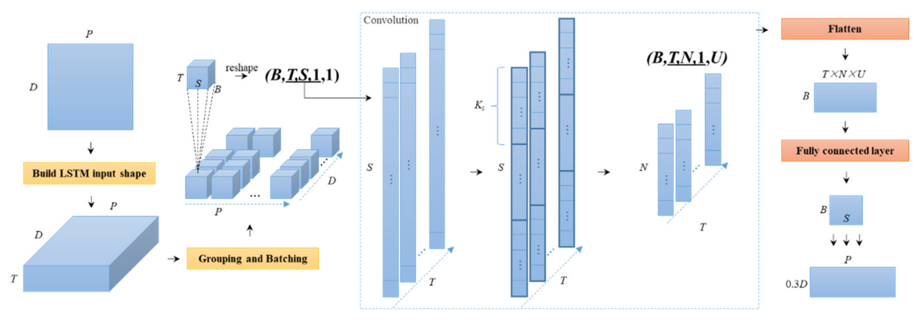
Figure 1. The structure of the ConvLSTM-F.
Jmse 10 00592 g001
Figure 2. The structure of the A-ConvLSTM.
Jmse 10 00592 g002
Figure 3. The structure of P-ATT model.
Jmse 10 00592 g003
Figure 4. The structure of the P-W-ATT model.
Jmse 10 00592 g004
Figure 5. The selected area of the East China Sea.
Jmse 10 00592 g005
Figure 6. The three points in the selected sea area.
Jmse 10 00592 g006
Figure 7. The comparison between the predicted OCs and observed OCs for spatial point (122.5° E, 30.25° N)—(a) u_current, (b) v current.
Jmse 10 00592 g007
Figure 8. The comparison between the predicted OCs and observed OCs for spatial point (129.875° E, 29.5° N)—(a) u_current, (b) v current.
Jmse 10 00592 g008
Figure 9. The comparison between the predicted OCs and observed OCs for spatial point (125.75° E, 27.125° N)—(a) u_current, (b) v current.
Jmse 10 00592 g009
Figure 10. The comparison between the predicted OCs and observed OCs with different ω for spatial point (129.875° E, 29.5° N)—(a) u_current, (b) v current. The subfigure (1) is the comparison result for August 2017. In order to clearly see the performance differences for different ω, we select several days from August and show the comparison results in subfigure (2).
Jmse 10 00592 g010aJmse 10 00592 g010b
Figure 11. (a) The comparison of MAE between different models—u_current, (b) The comparison of RMSE between different models—u_current, (c) The comparison of MAE between different models—v_current, (d) The comparison of RMSE between different models—v_current. The subfigure (1) is for all five models, the subfigure (2) is the comparison between CNN-GRU, ConvLSTM-F, and A-ConvLSTM, the subfigure (3) is the comparison between A-ConvLSTM and P-ATT, the subfigure (4) is the comparison between P-ATT and W-P-ATT, and the subfigure (5) is the comparison between P-ATT and W-P-ATT through a short point range from point 1520 to point 1550.
Jmse 10 00592 g011aJmse 10 00592 g011b
Figure 12. (a,b) The MAE and RMSE distributions for five models—u_current, (c,d) The MAE and RMSE distributions for five models—v_current. The subfigure (a) is MAE distribution for u_current and the subfigure (b) is RMSE distribution for u_current. The subfigure (c) is MAE distribution for v_current and the subfigure (d) is RMSE distribution for v_current.
Jmse 10 00592 g012
Figure 13. (a,b) The comparison between W-P-ATTs with different ω—u_current, (c,d) The comparison between W-P-ATTs with different ω—v_current. The subfigure (a) is MAE distribution for u_current and the subfigure (b) is RMSE distribution for u_current. The subfigure (c) is MAE distribution for v_current and the subfigure (d) is RMSE distribution for v_current.
Jmse 10 00592 g013
Table 1. The detailed information of the models.
ParameterCNN-GRUConvLSTM-FA-ConvLSTMP-ATTW-P-ATT
Kernel Size(5, 1)(5, 1)(5, 1)//
Stride(5, 1)(5, 1)(5, 1)//
Time Step/10
Input Shape(10, 2010, 1)(10, 2010, 1, 1)(10, 15, 1, 1)(10, 15)(10, 15)
No. of GRU Units256////
No. of Convolution filters256256256//
Batch Size32
Spatial Group Size//15
Spatial Scope23.625° N–31.375° N, 122.125° E–131.125° E
Training-time range1 January 2011 to 19 December 2015
Testing-time range20 December 2015 to 14 December 2017
Table 2. MAE, RMSE, and r for five different models; the values in bold mean the best results.
MetricsCNN-GRUConvLSTM-FA-ConvLSTMP-ATTW-P-ATT (ω = 0.7)
MAE (u_current)0.04340.03870.01720.00280.0017
RMSE (u_ current)0.05630.05080.02320.00610.0051
r (u_ current)0.62150.64990.90910.98990.9901
MAE (v_current)0.04680.04260.01450.00260.0014
RMSE (v_ current)0.06070.05570.01930.00590.0049
r (v_ current)0.58810.61550.92400.99080.9916
Publisher’s Note: MDPI stays neutral with regard to jurisdictional claims in published maps and institutional affiliations.