Time-Domain Implementation and Analyses of Multi-Motion Modes of Floating Structures

Abstract

The study of wave-structure interactions involving nonlinear forces would often make use of the popular hybrid frequency–time domain method. In the hybrid method, the frequency-domain analysis could firstly provide the reliable and accurate dynamic parameters and responses; then these parameters and responses are transformed to the parameters to establishing the basic time-domain equation. Additionally, with the addition of the required linear and nonlinear forces, the time-domain analysis can be used to solve for the practical problems. However, the transformation from the frequency domain to the time domain is not straightforward, and the implementation of the time-domain equation could become increasingly complicated when different modes of motion are coupled. This research presents a systematic introduction on how to implement the time-domain analysis for floating structures, including the parameter transformations from the frequency domain to the time domain, and the methods for calculating and approximating the impulse functions and the fluid-memory effects, with special attention being paid to the coupling terms among the different motion modes, and the correctness of the time-domain-equation implementation. The main purpose of this article is to provide relevant information for those who wish to build their own time-domain analyses with the open-source hydrodynamic analysis packages, although commercial packages are available for time-domain analyses.

1. Introduction

Frequency-domain analysis is a widely used method for wave-structure interactions and, in the method, the dynamic system is assumed to be fully linear: the governing equation is the linear Laplace equation (based on the incompressible potential flows); the body and seabed boundary conditions are linear; and the free-surface condition can be linearized for practical applications. Although the assumptions are strict, the frequency-domain analysis could provide reliable and accurate assessments for the hydrodynamic parameters and responses, such as the added mass, the radiation-damping coefficients, the wave-excitation forces, and the response amplitude operators (RAOs) [1,2,3,4,5], and, in some cases, it can be even extended to hydro-elastic analysis [6] and the elastic wave-energy converters (WECs) [7,8]. For its applications in wave-energy converters, the conventional frequency-domain analysis may provide an accurate calculation for the resonance frequency/period of the device, which is generally regarded as the most important parameter for wave-energy converters, since most wave-energy converters would be ideally optimized to have resonance with the wave for efficient energy extraction from the waves [9,10]. In addition, the frequency-domain analysis is also a powerful tool for optimizing WECs and power take-off (PTO) to maximize wave-energy production [11,12].

The assumption of fully linear dynamic systems in the frequency-domain analysis could limit its direct applications in WECs since, for some practical WECs, nonlinear PTO systems may be employed, such as hydraulic PTOs [13,14,15,16] or impulse turbines [17,18,19]. Additionally, when a control is applied to improve wave-energy conversion [20,21,22,23,24], the corresponding dynamic system in wave-energy conversion would be identically nonlinear, even if the PTO is linear. For a nonlinear dynamic system, the frequency-domain analysis can not be used directly; instead, the most applied method is the so-called hybrid frequency–time domain method [9,25,26,27]. In the hybrid method, the frequency-domain analysis is firstly used to obtain the relevant hydrodynamic parameters (that is, the frequency-dependent parameters), and these parameters and the frequency-domain equation are then transformed to the corresponding time-domain parameters and the Cummins’ time-domain equation [28]. To realize the transformation, the Ogilvie relation [29] is used for transforming the relevant frequency-dependent parameters to the parameters in the time domain, such as the impulse function, the fluid-memory effect, and the added mass at infinite frequency. For real problems, the transformed Cummins’ time-domain equation can be modified by adding the required forces (linear and/or nonlinear) for the actual problems.

However, such a transformation from the frequency domain to the time domain is not straightforward. It involves the transformation from the frequency-dependent radiation-damping coefficients to the impulse functions and the subsequent fluid-memory effects to represent the fluid-damping effects on the floating structures, and the transformation from the frequency-dependent added mass to the added mass at infinite frequency. Additionally, to calculate the memory effects more effectively, the impulse functions are frequently approximated, so are the fluid memory effects [30,31,32].

The transformations and approximations would become increasingly complicated when different modes of motion are coupled together [12] (compared to those time-domain analyses of the single-motion mode, such as on heave [9], or on pitch [26,27]). However, in reality, the multiple motion modes must be analyzed for some floating structures and WECs, for instance, the multi-axis WECs [16]. The current research systematically presents and explains how the correct transformations can be made, how the memory effects are approximated, and how the multiple coupled motions are solved. Moreover, a validation method is introduced, which would allow the researchers to check whether the numerical modeling implementation for the time-domain modeling is correct. When this important step is completed, the researchers can be more confident to add the required forces to the dynamic equation for the practical problems.

The rest of the paper is arranged as follows: Section 2 presents a brief introduction of the multi-axis TALOS WECs; Section 3 introduces the frequency-domain equation and responses, paying attention to the coupled-motion modes of the TALOS WECs; Section 4 establishes the time-domain analysis, introducing how to transform the frequency-domain equation into the time-domain equation; Section 5 presents the methods for approximating the impulse function and the memory effect of the fluid on the structure; Section 6 discusses the implementation and validation method of the time-domain analysis; and, finally, in Section 7, the conclusions are presented regarding the implementation of the time-domain analyses for floating structures.

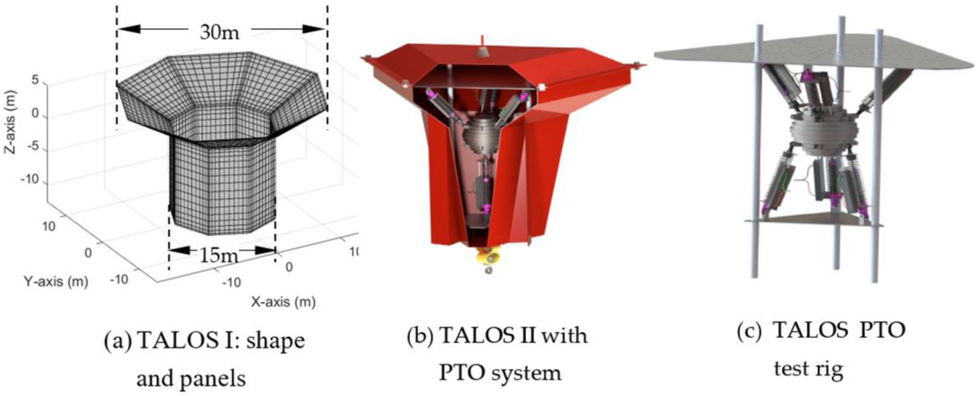
2. TALOS WEC

TALOS is a point absorber-type WEC, which was proposed and initially developed at Lancaster University, UK [16]. The general shape for TALOS I is an octagonal-shaped floating structure (see the panels of the wet surfaces of the TALOS in Figure 1a), and it was the target floating structure in this research for studying the wave-structure interaction and the implementation of the time-domain analysis for the multiple-motion modes of a floating structure.

The TALOS WEC is a wave-energy converter with a multi-axis PTO system, which consists of a heavy ball enclosed in the wave-energy converter, supported with the springs and dampers, see the PTO system in TALOS II from the cut-off in Figure 1b, and the multi-axis PTO test rig (Figure 1c). This multi-axis wave-energy converter converts wave energy from the multiple-motion modes of the structure in waves for a more efficient wave-energy extraction. In converting the wave energy, the heavy ball remained relatively stationary while the structure motions under the wave excitation induced the relative motion between the structure and the heavy ball to drive the PTOs (including the springs and dampers) to convert the wave energy into useful mechanical energy. As a result of such an arrangement, the TALOS WEC had the advantage of being a multi-axis wave-energy converter (the other advantages of the TALOS WEC include the fully enclosed PTO in the structure, thus affording a good survivability for the WEC device).

Recently, the TALOS multi-axis wave-energy-converter technology (the project’s short name: ‘NHP-WEC’) was selected as one of eight projects supported by UK Research and Innovation (UKRI) [33], which aim to unlock the potentials of marine wave energy. The main focuses of the NHP-WEC project are to optimize the TALOS WEC and the relevant PTO system, as well as to advance WEC technology by developing the essential device control and monitoring systems that are integrated with high-fidelity sea-state forecasting using the SmartWave toolset [34]. The current work is part of the ongoing research of the NHP-WEC project, an important step towards the implementation of the numerical model for the multi-axis TALOS wave-energy technology.

3. Frequency-Domain Governing Equation and Responses

3.1. Frequency-Domain Governing Equation

Frequency-domain analysis is a very popular method for the wave-structure interactions [35,36,37], in which the governing equation for wave-structure interactions is solved in the frequency domain, with the relevant hydrodynamic parameters (added mass, radiation-damping coefficient, and wave excitation) being assessed using the panel method, such as the open source, HAMS (Hydrodynamic Analysis of Marine Structure [38]), and the commercial package, WAMIT [39]. The panel method for wave-structure interaction is based on the potential flow theory and solves for the problems of wave-structure interactions under the assumption of the dynamic system being fully linear. These assumptions seem very strict, but the panel method is in fact very reliable and accurate for a large range of practical problems, while, for many other problems of wave-structure interactions, it could still provide the required hydrodynamic parameters reliably for further analyses, including the time-domain analyses as the time-domain implementation in this research.

The main purpose here is to implement time-domain modeling based on the predictions of the open-source panel method, HAMS. However, for the purpose of basic validations, the commercial code, WAMIT (widely regarded as an industrial standard for studying wave-structure interactions), was employed for the purpose of comparisons (more detailed comparisons between HAMS and WAMIT can be found in [40]). Here, the comparisons between HAMS and WAMIT were made to simply check the correctness of the relevant frequency-dependent parameters and of the corresponding impulse functions.

Following WAMIT [39], the frequency-domain governing equation of 6-degrees-of-freedom (DOFs) motions of a rigid structure is presented in a form of a mass-spring-damper system, as

$${\displaystyle \sum }_{k=1}^6\left\{-{\omega }^2\left[M_{jk}+M_{ij}^E+A_{jk}\left(\omega \right)\right]+i\omega \left[B_{jk}\left(\omega \right)+B_{jk}^E\right]+\left(C_{jk}+C_{jk}^E\right)\right\}{\xi }_k\left(\omega \right)=F_j^{ }\left(\omega \right)$$

(1)

where

ω is the circular frequency of the wave excitation, and the parameters with the variable ω represent their frequency dependency.

$M_{jk}, M_{jk}^E,A_{jk}\left(\omega \right) \left(j, k=1, 2, \dots , 6\right)$ are the structure and external and added-mass matrices, and the former two must be specified for the numerical modeling, while the latter can be assessed using the panel method. In some wave-energy converters, the external-mass matrix $M_{jk}^E$ may be from the generic PTO, see Babarit [41].

$B_{jk}\left(\omega \right), B_{jk}^E \left(j, k=1, 2, \dots , 6\right)$ are the radiation and external-damping coefficients, with the former being assessed using the panel method, while the latter must be specified in the numerical modeling; the external-damping coefficient $B_{jk}^E$ may be from the generic PTO as above or from other linear dampings.

$C_{jk}, C_{jk}^E \left(j, k=1, 2, \dots , 6\right)$ are the structure hydrostatic and external restoring coefficients (both must be specified or calculated). The definition of the hydrostatic restoring coefficients $C_{jk}$ can be found in the WAMIT manual [39]; the external restoring coefficient $C_{jk}^E$ may be from the PTO or from the linearized mooring system.

$F_j^{ }\left(\omega \right)\left(j=1, 2, \dots , 6\right)$ is the frequency-dependent complex amplitude of the wave excitation, which can be calculated using the panel method.

${\xi }_k\left(\omega \right)\left(k=1, 2,\dots , 6\right)$ corresponds to the motions of surge, sway, heave, roll, pitch, and yaw, respectively, as the frequency-dependent complex amplitudes of motions for the floating structure. Additionally, these are solved from the above governing equation and, as a convention, the response amplitude operator (RAO) is a more useful expression, defined as

$${\chi }_k=\frac{{\xi }_k}{A}$$

(2)

where A is the wave amplitude (here, the wave amplitude A is without a subscript or superscript). Obviously, in the wave of a unit amplitude, the frequency-dependent ${\xi }_k$ itself is the RAO.

In the conventional plots, the module of the RAO may be seen more often, which is defined as

$$\left|{\chi }_k\right|=\frac{\left|{\xi }_k\right|}{A}$$

(3)

From the terms regarding the added mass, the radiation damping and the restoring coefficients in Equation (1), we can observe that the motions of a free-floating structure may couple together through the cross-coupling coefficients. The motion couplings can be either through the wave radiation, that is, through the cross-coupling added-mass and radiation-damping coefficients, such as $A_{15}$ (as the surge-pitch coupling), $B_{24}$ (the sway-roll coupling), if these coupling coefficients are not zero, nor very small when compared to other terms, say, $A_{11}$ and $B_{22}$; or, through the coupling hydrostatic restoring coefficients, for instance, the coupled restoring coefficients between heave and roll (pitch), as $C_{34}$ or $C_{35}$. It should be noted that some of the coupled motions are inherently existing, e.g., surge-pitch coupling and sway-roll coupling, while some other coupled motions may exist or not, very much depending on the shape of the floating structure, for instance, a structure with a symmetry about x axis may lead to the de-coupling of the heave and pitch motions.

In the following subsections, the hydrodynamic parameters and responses are presented and discussed for the TALOS floating structure, and the comparisons between HAMS and WAMIT aim to confirm that the open-source panel method, HAMS, is reliable and accurate.

3.2. Added Mass

The conventional added mass of the TALOS wave-energy converter is presented in Figure 2, including the added mass for surge ($A_{11}$), sway ($A_{22}$), heave ($A_{33}$), roll ($A_{44}$), pitch ($A_{55}$), and yaw ($A_{66}$). We can observe from the comparisons between HAMS and WAMIT that they are almost identical, and some differences (spikes) can be observed in the so-called irregular frequencies in the short waves, when the wave period, $T$, is less than 3 s. The reason for the irregular frequencies may relate to the panel size: as a rule of thumb, the maximal panel size should be less than 1/8 of the wave length (see [37]).

However, the spiky responses of the short waves (of high frequencies) would have no significant influence on the performance of the floating structure (see the smooth-motion responses, the RAOs in Section 3.5), or in the interest for wave-energy extraction due to the corresponding low-wave-energy density of short waves.

For the free-floating structure, TALOS, we can observe that there are some strong couplings between the motions in terms of the added mass, such as the surge pitch (see $A_{15}$, Figure 3a) and sway roll (see $A_{24}$, Figure 3b). It can also be noted that, due to the symmetry of the couplings, $A_{51}=A_{15}$, and $A_{42}=A_{24}$, and also the corresponding added mass of the strong coupling terms, which have a similar order of magnitude as the conventional added mass (compared to Figure 2a,b). Here, we can observe that $A_{24}$ is a negative added mass, which means that the motion of the roll would produce an added mass on the sway in an opposite phase. Obviously, in the applications, these strong coupling terms must be included in both the frequency-domain and time-domain analyses.

For a comparison, we also present the weak couplings in the heave pitch (see $A_{35}$, Figure 3c), and, here, we can observe that they are quite different in relation to the HAMS and WAMIT predictions, probably due to the slightly different methods employed to approximate the free-surface Green function. However, the magnitude of the added mass for the weak couplings would be several orders smaller than the conventional added mass (~300 vs. 3 × 10⁶). Therefore, the weak coupling terms can be fully omitted in the numerical modeling since these terms would not have any influence on the overall performance of the structure motions and responses, although such a weak coupling presented between the heave and pitch of TALOS may be an indication that the heave and pitch could be strongly coupled if a different structure, for instance, a floating structure with no symmetry for the y axis was applied (here, TALOS has 2 symmetries for the x and y axes, respectively).

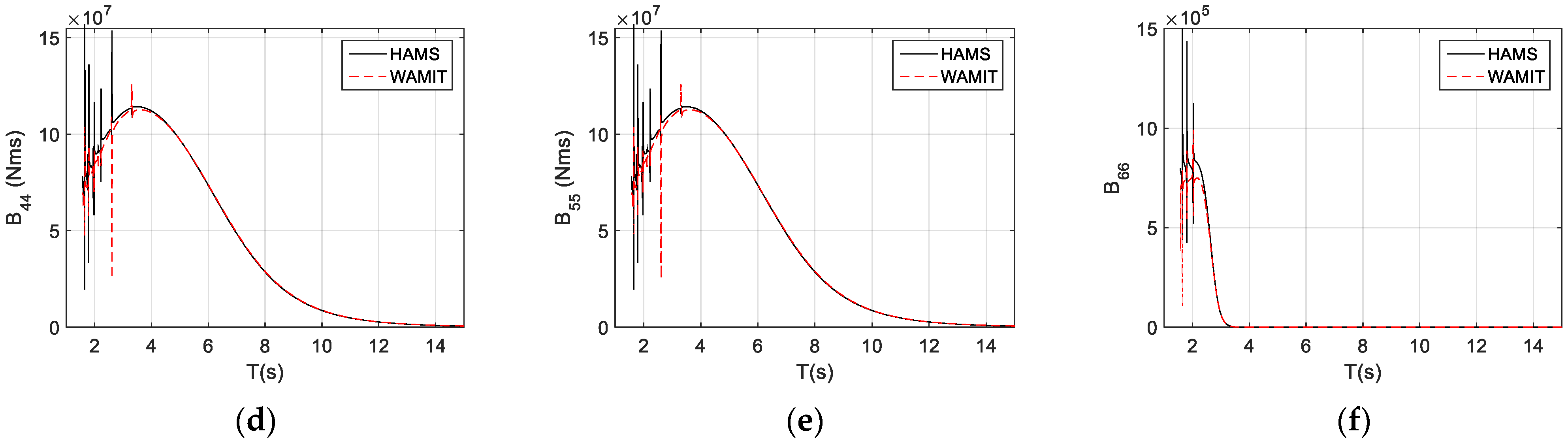
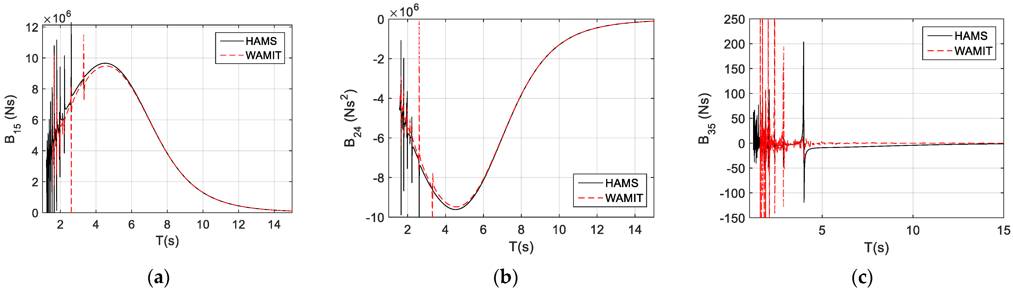
3.3. Radiation-Damping Coefficients

The conventional radiation-damping coefficients of the TALOS wave-energy converter are presented in Figure 4. These include the radiation-damping coefficients, $B_{11}$ for surge, $B_{22}$ for sway, $B_{33}$ for heave, $B_{44}$ for roll, $B_{55}$ for pitch, and $B_{66}$ for yaw. Again, we can observe that the results from HAMS and WAMIT are almost identical, with differences at the irregular frequencies in the short waves (the wave periods, $T$, less than 4 s). Again, these irregular frequencies are due to the limited panel size, similar to the cases in the added mass.

Similarly, we can observe that there are some strong couplings between the motions, such as surge pitch (see $B_{15}$, Figure 5a) and sway roll (see $B_{24}$, Figure 5b), and these coupling terms would correspond to those of the strong coupling terms on added mass. These strongly coupled radiation-damping coefficients would have similar orders of magnitude as those conventional radiation-damping coefficients (refer to Figure 4a,b). One interesting factor is that the coupled radiation-damping coefficient can be negative, for instance, the coupled radiation-damping coefficients for sway and roll, $B_{24}$ (Figure 5b), which is very different from the positive conventional radiation-damping coefficient. This can be understood as follows: in the conventional radiation-damping coefficients, the self-radiation would simply radiate the wave away due to the structure motion, and dissipate the energy from the moving structure, hence the radiation-damping coefficient must be positive; while in the coupled damping coefficients, for instance, $B_{24}$, which is the damping coefficient due to the radiated wave from the roll motion (the subscript ‘4’) contributing to the damping effect on the sway motion (the subscript ‘2’), the coupling effect is in an opposite phase, hence it is physically negative (for a comparison, $B_{15}$ is positive, see Figure 5a).

Similarly, we can observe the weak coupling presented in the heave pitch (see $B_{35}$, Figure 5c). Again, the magnitude of the radiation-damping coefficient for the weak coupling is a few orders smaller than the conventional radiation-damping coefficient (~200 vs. 2 × 10⁶). Therefore, the weak coupling terms can be omitted from the numerical modeling. In fact, in the corresponding time-domain analysis, such weak coupling terms must be dropped; otherwise, it may cause divergence problems in the numerical modeling due to the possibly corresponding divergent-impulse functions (the details are discussed later in the research).

3.4. Wave Excitation

Wave-excitation forces are dependent on both the floating structure itself and the direction of the incoming waves. Here, an angle of 45° for the incoming wave was used for calculating the wave excitations acting on the structure. From Figure 6, we can observe the wave-excitation responses (under the waves of unit amplitude) for different motion modes (surge, $F_{ex1}$; sway, $F_{ex2}$; heave, $F_{ex3}$; roll, $F_{ex4}$; pitch, $F_{ex5}$; and yaw, $F_{ex6}$). Additionally, the wave excitations for surge and sway are the same (Figure 6a,b) in such a wave condition (45°) and due to the symmetry of the TALOS structure. Additionally, for the same reason, the excitations for roll and pitch are the same (see Figure 6d,e).

The excitations for the surge, sway, roll, and pitch all have maximums at certain wave periods (see Figure 6a,b,d,e), while the excitation for the heave monotonically increases in short waves (Figure 6c), and its increase is in long waves, but in very long waves, the increase would be small. The reason for these is because the excitations for the surge, sway, roll, and pitch are all dependent on the slope of the wave, while the excitation for heave is dependent on the dynamic pressure acting on the bottom of the structure, thus it will be greater in longer waves. Therefore, the excitation for heave increases with the longer waves.

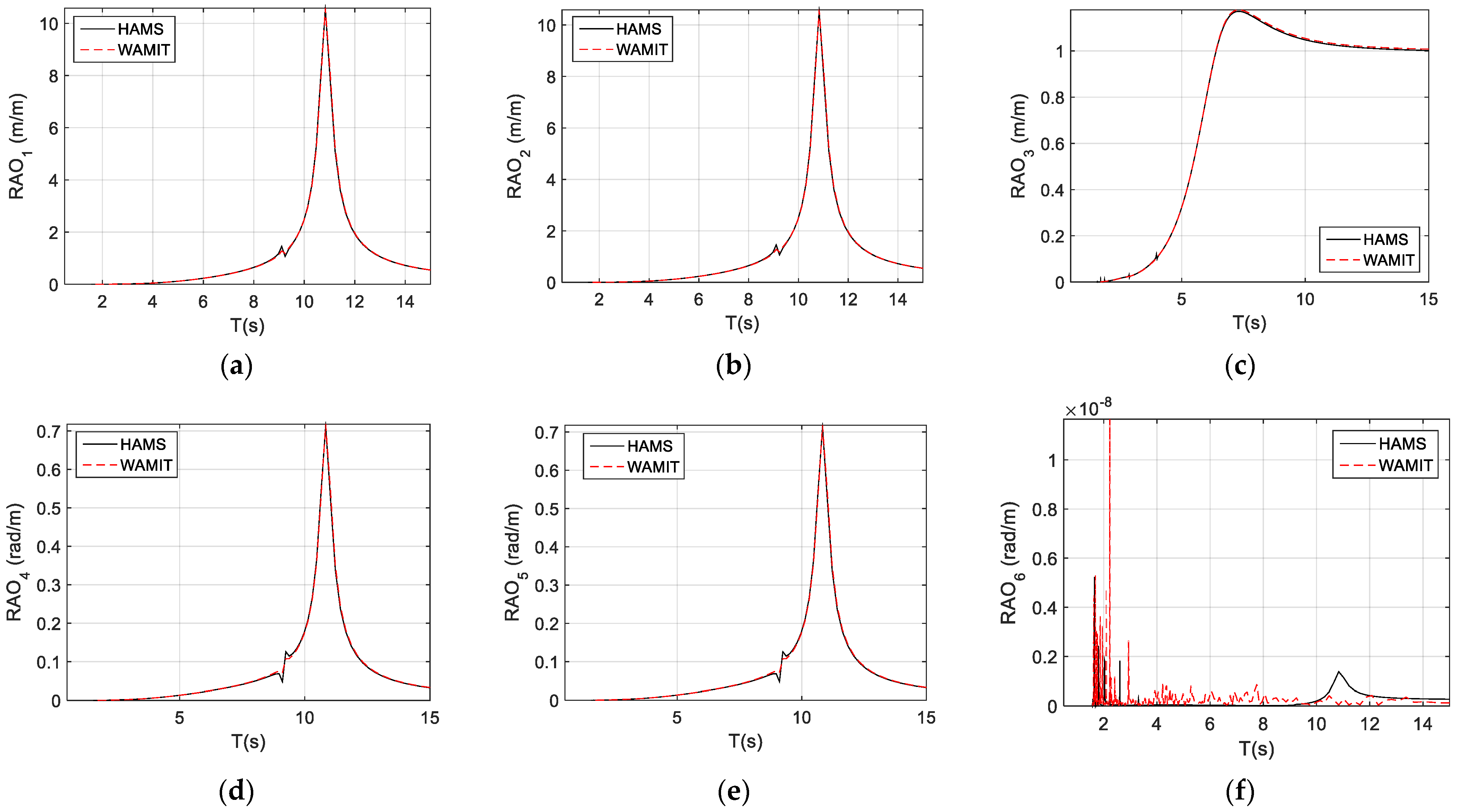
3.5. Response Amplitude Operators (RAOs)

For the free-floating marine structures, only three motion modes (out of six DOFs) had inherent restoring forces: heave, roll, and pitch, and the latter two motions would also be very dependent on the position of the center of gravity of the structure. In the current modeling, the center of gravity was set at $z_g=-5.0 m$ (that is, 5.0 m below the water’s surface).

For the other three motion modes (surge, sway, and yaw), there were no inherent restoring forces. Hence, for most floating structures, the required restoring forces/moments must be provided by the mooring system to the structure or other means. Here, for simplifying the analysis, we assumed the linear restoring coefficients for the surge, sway, and yaw motions to be: $C_{11}=C_{22}$ = 2.5 × 10⁶ N/m and $C_{66}$ = 5 × 10⁶ Nm (and these added restoring coefficients mean a relatively stiff mooring system). It should be noted that these linear restoring coefficients can be obtained by linearizing the mooring forces, and the linearization of the mooring forces can be valid if the structure motions are small in magnitude.

Under the above mooring setting, the surge and sway motion responses are the same, as can be observed in Figure 7a,b, due to the symmetrical TALOS and the same added restoring-force coefficients for the surge and sway. The large responses presented in Figure 7a,b at T = 10.83 s correspond to the resonance period of the surge and sway, respectively, while the very small responses at T = 9.24 s are due to the respective responses of the pitch and roll motions.

From Figure 7c, it can be observed that the heave motion response would only be dependent on the structure itself, and the resonance period is T = 7.22 s, while for the roll and pitch (Figure 7d,e), their responses are identical, simply due to the symmetrical structure of the TALOS and incoming wave (45°). The roll and pitch have large responses at the resonance period of T = 10.83 s due to the couplings of the surge and sway, and the small responses at period T = 9.24 s, which would correspond to the resonances of the roll and pitch motions.

For the yaw response, due to the symmetries of the TALOS structure (a nearly axi-symmetrical structure), it is very small, so small as an effective zero (see Figure 7f).

4. Time-Domain Dynamic Equation and Analysis

4.1. Dynamic Equation

The time-domain dynamic equation is in fact the dynamic equation based on Newton’s second law of motion for multiple motion modes of a rigid body, and, generally, this dynamic equation is written in the form of mass-spring-damper, with the damping force and the restoring force acting on the structure being moved to the left-hand side. With the inclusions of the wave-radiation forces, wave excitation as well as the additional external forces, the dynamic equation would be presented as:

$$\begin{gathered} {\displaystyle \sum }_{k=1}^6\left\{\left[M_{jk}+M_{jk}^E+A_{jk}\right]{\ddot{x}}_k\left(t\right)+\left[B_{jk}+B_{jk}^E\right]{\dot{x}}_k\left(t\right)+\left(C_{jk}+C_{jk}^E\right)x_k\left(t\right)\right\}=f_j^{ }\left(t\right) \\ (j=1, 2, \dots , 6) \end{gathered}$$

(4)

where

$x_k\left(t\right)$ (k = 1, 2, …, 6) are the 6-DOF motions of the structure in the time domain.

$f_j\left(t\right)$(j = 1, 2, …, 6) is the time-domain wave-excitation force, which can be calculated based on the wave-excitation response from the panel method analysis.

For a linear dynamic equation, that means, the mass matrices, the damping-coefficient matrices and the restoring-coefficient matrices are all independent of the motions. Additionally, under a sinusoidal excitation, for instance, $f_j\left(t\right)=F_j{e}^{i\omega t}$ (here, $F_j$ is a complex amplitude of the jth wave excitation), the motion would be sinusoidal too, then we shall have the following relations:

Motion: $x_k\left(t\right)={\xi }_k{e}^{i\omega t}$ Velocity: ${\dot{x}}_k\left(t\right)=i\omega {\xi }_k{e}^{i\omega t}$

Acceleration: ${\ddot{x}}_k\left(t\right)=-{\omega }^2{\xi }_k{e}^{i\omega t}$

where ${\xi }_k$ is the complex amplitude of the motion.

Substituting the above relations into Equation (4), and dropping the time factors in all terms, we can obtain the frequency-domain equation, which would be exactly same as in Equation (1). However, it should be noted that, when transforming the frequency-domain Equation (1) back to the time-domain Equation (4), we should be very careful in determining the frequency-dependent added-mass and radiation-damping coefficients.

The direct transformation from Equation (1) to Equation (4) can only be correct if the dynamic system is linear and under a sinusoidal excitation, because in such a dynamic system, the excitation and motions are all sinusoidal (i.e., of single frequency), hence the frequency-dependent parameters, $A_{jk}$, $B_{jk}$ and $F_j$, can be determined and all clearly have a physical significance, as does the time-domain Equation (4).

However, such a fully linear dynamic system is not the purpose of employing the time-domain approach, and this is especially true for most wave-energy converters. For instance, to examine the wave-energy converter’s performance in irregular waves, the excitation and the motions in irregular waves would all have multi-frequencies. As such, the frequency-dependent terms, $A_{jk}$ and $B_{jk}$, become undecided, although the time-domain excitation is calculated, see Equation (6) below. A more general case is that the wave-energy converter may include some nonlinear forces in the dynamic system, such as the force from the nonlinear PTO or the force from the PTO control for improving wave-energy extraction, or the nonlinear forces from the mooring system; the motions would surely be have multiple frequencies, even if the excitation is sinusoidal. As such, $A_{jk}$ and $B_{jk}$ become undetermined too.

The most used time-domain equation for the wave-structure interaction would be the Cummins’ time-domain equation [28] with the Ogilvie relation [29], namely, the hybrid frequency–time domain method, according to [25], and the time-domain equation has the following form:

$$\begin{gathered} {\displaystyle \sum }_{k=1}^6\left\{\left[M_{jk}+M_{jk}^E+A_{jk}(\infty )\right]{\ddot{x}}_k\left(t\right)+{{\displaystyle \int }}_0^t{K}_{jk}\left(t-\tau \right){\dot{x}}_k\left(\tau \right)d\tau +B_{jk}^E{\dot{x}}_k\left(t\right)+\left(C_{jk}+C_{jk}^E\right)x_k\left(t\right)\right\}=f_j^{ }\left(t\right)+f_j^E\left(t\right) \\ (j=1, 2, \dots , 6) \end{gathered}$$

(5)

where

$x_k\left(t\right)$ (k = 1, 2, …, 6) are the structure motions (the motions of 6 DOFs of the structure, which would be solved in the dynamic equation);

$A_{jk}(\infty ) \left(j, k=1, 2, \dots , 6\right)$ is the added-mass matrix at infinite frequency, which can be assessed using the frequency-domain analysis data (see the next section);

$K_{jk}\left(t\right)$ (j, k = 1, 2, …, 6) is the impulse function, which would be calculated based on the frequency-domain results (see the next section);

The parameters with superscript ‘^E’ are the parameters/forces externally added to the dynamic system, such as $f_j^E\left(t\right)$ (j = 1, 2, …, 6) the external force, for instance, the force from power take-off (PTO), or the control force, or the force from the mooring system, and these forces can be both linear and nonlinear.

$f_j\left(t\right)$(j = 1, 2, …, 6) is the wave-excitation force in an irregular wave of a given wave spectrum. The corresponding wave-excitation force can be calculated using the frequency-dependent wave-excitation responses, $F_j$. The time-domain wave excitation is calculated as

$$f_j^{ }\left(t\right)={\displaystyle \sum }_{n=1}^{\infty }{F}_j\left({\omega }_n\right)e^{i{\omega }_{n}t}{A}_n{e}^{i{\epsilon }_n}={\displaystyle \sum }_{n=1}^{\infty }{F}_j\left({\omega }_n\right)A_n{e}^{i\left({\omega }_{n}t+{\epsilon }_n\right)}$$

(6)

where

$F_j\left(\omega \right)$ is a complex wave-excitation response (assessed using the panel method);

${\epsilon }_n$ is the random phase for the wave components in an irregular wave;

$A_n$ is the wave amplitude of the wave component corresponding to the frequency ${\omega }_n$ (of a bandwith $\Delta {\omega }_n)$, calculated as

$$A_n=\sqrt{2S\left({\omega }_n\right)\Delta {\omega }_n}$$

(7)

with $S\left(\omega \right)$ being the wave spectral density, such as the popular wave spectra, Bretschneider or JONSWAP spectrum [42].

4.2. Memory Effect and the Impulse Functions

In the transformation from frequency domain to time domain, the relevant frequency-dependent parameters must be transformed accordingly, including the added mass and the radiation damping coefficients, while the wave excitation in irregular waves can be assessed in Equation (6).

From the Cummins’ time-domain equation, the frequency-dependent damping terms in the frequency-domain equation are all replaced using the corresponding convolution terms, or, more specifically, the memory effects, due to the relevant fluid motions. The memory effect is presented in a convolution term as

$$I_{jk}\left(t\right)={{\displaystyle \int }}_0^t{K}_{jk}\left(t-\tau \right){\dot{x}}_k\left(\tau \right)d\tau$$

(8)

Accordingly, in the Cummins’ time-domain equation, the added mass at infinite frequency, $A_{jk}(\infty )$, replaces the frequency-dependent added mass in the frequency-domain equation, see Equation (5).

4.3. Impulse Function

Based on the Ogilvie relation [29], the impulse function for the wave-structure interaction can be calculated from the frequency-dependent radiation-damping coefficients, $K_{jk}$, given as

$$K_{jk}\left(t\right)=\frac{2}{\pi }{{\displaystyle \int }}_0^{\infty }{B}_{jk}\left(\omega \right) cos\omega t d\omega$$

(9)

In the numerical modeling, the sampled impulse function can be obtained from the sampled radiation-damping coefficient (here, the subscripts are dropped for a simplicity of the expression), calculated as

$$K\left(t_m\right)=\frac{2}{\pi }{\displaystyle \sum }_{n=1}^{N}B\left({\omega }_n\right) cos\left({\omega }_n{t}_m\right) \Delta {\omega }_n$$

(10)

where N is the total number of the frequencies in the frequency-domain analysis, and m = 1, 2, …, M is the number of the sampled impulse function, with a time interval $\Delta t$, and the time series is presented as $t_m=\left(m-1\right)\Delta t$. One can observe that the calculation of the impulse function is from a low frequency to a reasonably high frequency, not necessarily from zero to infinite frequency (note: the radiation-damping coefficient is asymptotic to zero on both sides of the wave frequencies). A MATLAB function for calculating the impulse function can be found in Appendix A.

In the numerical modeling, based on the assessment of the frequency-domain radiation-damping coefficients, we can use Equation (10) to calculate the impulse function and, for the purpose of validation, WAMIT F2T utility was used to obtain the impulse function [39]. Figure 8 shows the comparisons of the results calculated from the HAMS radiation-damping coefficients, as described above, and the results obtained from WAMIT F2T for the conventional impulse functions, $K_{11},K_{22},K_{33},K_{44}, K_{55}, K_{66}$. It can be observed that they are all almost identical between the results obtained for HAMS and WAMIT.

When we examined the dynamically coupling terms between the different motion modes, we observed the coupling terms between the surge pitch, $K_{15}$, and sway roll, $K_{24}$(see Figure 9a,b). These were strong coupling terms, since their magnitudes would be in orders similar to those of the conventional impulse functions. In comparison, the impulse functions for the strong coupling terms from HAMS and WAMIT were almost identical.

Figure 9c shows a weak coupling between the heave and pitch, $K_{35}$. Here, we can observe a great difference between HAMS and WAMIT, and also the weak coupling impulse functions are very different from those of the conventional impulse functions: the weak coupling impulse function can be divergent.

Having observed the great differences, their magnitudes are essentially much smaller than the conventional impulse functions ($~10 \mathrm{vs}. {10}^6$). In fact, for a practical purpose, these weak coupling terms must be dropped in the numerical modeling, otherwise it may cause a divergence problem in the time-domain calculations due to the divergent impulse function.

4.4. Added Mass at Infinite Frequency

Once the impulse function has been calculated, the added mass at infinite frequency can the be assessed as

$$A(\infty )=A\left(\omega \right)+\frac{1}{\omega }{{\displaystyle \int }}_0^{\infty }K\left(\tau \right) sin\omega \tau d\tau$$

(11)

In a discretized form, for a given frequency,${\omega }_n$, the added mass at infinite frequency is calculated as

$$A_n(\infty )=A\left({\omega }_n\right)+\frac{1}{{\omega }_n}{\displaystyle \sum }_{m=1}^{M}K\left({\tau }_m\right) sin\left({\omega }_n{\tau }_m\right) \Delta \tau$$

(12)

In principle, the added mass at infinite frequency can be calculated based on a given frequency, say ${\omega }_n$. However, due to the possible errors in the numerical modeling, such as irregular frequencies, a more reliable calculation for the added mass at infinite frequency is to average the added mass at infinite frequency based on the corresponding multiple frequencies, ${\omega }_1, {\omega }_2, {\omega }_3,\dots$,${\omega }_N$, as

$$A(\infty )=\frac{1}{N}{\displaystyle \sum }_{n=1}^N{A}_n(\infty )$$

(13)

Using the above method, we can calculate the added mass at infinite frequency based on the frequency-dependent added mass and the calculated impulse function (see also Appendix A).

Table 1. A comparison of added mass at infinite frequency.

Added Mass	WAMIT	Calculation	Error (%)
$A_{11 }$(kg)	2.047 × 106	2.040 × 106	−0.338
$A_{15}$(Ns2)	1.582 × 106	1.620 × 106	2.430
$A_{33}$(kg)	2.583 × 106	2.580 × 106	−0.116
$A_{55}$(Nms2)	1.353 × 108	1.360 × 108	0.517

shows the comparison of the added mass at infinite frequency from the HAMS calculation and the assessment using WAMIT. Here, we can observe that they are very close, especially for the conventional added mass at infinite frequency, with an error less than 0.5%, while a slightly large difference occurs for the coupled added mass A₁₅, with an error of about 2.5%. Hence, we can conclude that all the errors should be within the acceptable range in the engineering calculations.

5. Approximations of Impulse Function and Memory Effect

5.1. Approximation of Impulse Function

Generally, the normal impulse function $K\left(t\right)$ would be a decayed function, which would converge to zero with time. This feature of the impulse function corresponds to the fluid-memory effect in physics: the events closer to the current time would have a greater influence on the current motion, and with time lapsing further, the influence becomes less and less, and eventually fades to zero (that is, $K\left(t\right)=0$ when $t$ is large).

There are generally two different ways to approximate such impulse functions, namely, the Prony approximation method [31,32,43] and the state-space method [30]. Here, the Prony function approximation was employed, because the Prony function has a more straightforward physical meaning for approximating the impulse function.

Following Duclos et al. [31], the impulse function can be approximated using the Prony function in the following form:

$$K\left(t\right)\approx {\displaystyle \sum }_{k=1}^{N_0}{\alpha }_k{e}^{{\beta }_{k}t}$$

(14)

where $N_0$ is the order of the Prony function, and the complex coefficients ${\alpha }_k$ and ${\beta }_k$ can be obtained from the Prony method. For a convergent impulse function, the real part of the parameter, ${\beta }_k$, must be negative. If it is not, the corresponding term must be dropped since it is divergent in nature (a MATLAB function for obtaining ${\alpha }_k$ and ${\beta }_k$ from the impulse function, $K\left(t\right)$, can be found in Appendix B).

Figure 10 shows the approximations of the impulse functions for the self-radiations; here, $N_{0 }$ = 10 (that is, the 10th order Prony function was used). It can be observed that all the impulse functions have been well reproduced. Figure 11 shows the impulse functions for the strong coupled terms, such as $K_{15}$ (note: $K_{51}$ is symmetric to $K_{15}$) and $K_{24}$. Again, these impulse functions have been well reproduced by the Prony approximations.

For the weak coupling terms, such as $K_{13}$, $K_{35}$, and $K_{46}$ (Figure 12), it seems more difficult to reproduce the weak impulse functions, though $K_{35}$ seems good (Figure 12b). Since these weakly coupled impulse functions are unlike the well-convergent normal impulse functions, they may not decay with time (Figure 12a,c), or simply diverge with time (Figure 12b). For such impulse functions, the Prony method would not correctly reproduce the impulse function due to the omission of the terms when the real part of ${\beta }_k$ is positive (see Figure 12b).

However, if these weak impulse functions are compared to the strong coupled impulse functions, their magnitudes could be many orders smaller than the strong coupling terms, for instance, $K_{35}$ ~10 vs. $K_{15}$ ~${10}^6$. Thus, in numerical modeling, these weak coupled impulse functions must be dropped to ensure the convergent solution in the time-domain analysis, while these small amplitude impulse functions have no influence on the overall motions of the structure.

The order of the Prony function, $N_0$, would be an important factor to determine how accurately the impulse functions can be approximated. Taking $K_{33}$ as an example, we can determine the differences using different orders of the Prony function to approximate the impulse function (Figure 13): $N_0$ = 6 is quite good, while $N_0$ = 5 seems much worse; $N_0$ = 8 could provide a much closer approximation, while for $N_0$ = 10, the approximation would be almost identical to the original impulse function.

5.2. Calculation of the Memory Effect

Substituting the Prony approximation, Equation (14), to the formula of the memory effect, Equation (8), yields

$$I\left(t\right)\approx {{\displaystyle \int }}_0^t{\displaystyle \sum }_{k=1}^{N_0}{\alpha }_k{e}^{{\beta }_k\left(t-\tau \right)}\dot{x}\left(\tau \right)d\tau ={\displaystyle \sum }_{k=1}^{N_0}{\alpha }_k{e}^{{\beta }_{k}t}{{\displaystyle \int }}_0^t{e}^{-{\beta }_k\tau }\dot{x}\left(\tau \right)d\tau ={\displaystyle \sum }_{k=1}^{N_0}{I}_k\left(t\right)$$

(15)

in which the order of integral and summation has been swapped, and

$$I_k\left(t\right)={\alpha }_k{e}^{{\beta }_{k}t}{{\displaystyle \int }}_0^t{e}^{-{\beta }_k\tau }\dot{x}\left(\tau \right)d\tau$$

(16)

Up to here, the calculation of the memory effect would be concentrated on how well and how fast we can calculate or solve for $I_k\left(t\right)$ (k = 1, 2, …, N₀). Subsequently, two different ways to solve $I_k\left(t\right)$ would be introduced.

(1)

Method ‘1’: solving additional differential equations [31]

Taking a differentiation of $I_k\left(t\right)$ with regard to t, we obtain

$${\dot{I}}_k\left(t\right)={\beta }_k{\alpha }_k{e}^{{\beta }_{k}t}{{\displaystyle \int }}_0^t{e}^{-{\beta }_k\tau }\dot{x}\left(\tau \right)d\tau +{\alpha }_k{e}^{{\beta }_{k}t}\left[e^{-{\beta }_{k}t}\dot{x}\left(t\right)\right]={\beta }_k{I}_k\left(t\right)+{\alpha }_k\dot{x}\left(t\right)$$

(17)

where the expression in the square brackets is a differentiation of the integral in Equation (16) with regard to time, t.

Obviously, Equation (17) is an actual first-order differential equation for $I_k$. In the classical Prony method [31], these first-order differential equations are simply added to the dynamic equations for solving $I_k$, when solving for the motions of the structure. Once $I_k$ is solved, the memory effect can be calculated using Equation (15).

In the numerical modeling using the classical Prony method, if multiple motion modes are involved, the number of the additional differential equations would be large. For example, taking 2 coupled motions (say, surge-pitch coupling), we would have 4 memory-effect terms ($K_{11}$, $K_{15}$, $K_{51}$, and $K_{55}$). Now, if we use a 10th-order Prony function, then we would have a total of 40 additional first-order differential equations, added to 2 s-order dynamic equations for the motions (i.e., surge and pitch). If we write the second-order differential equation in the form of first-order differential equations, we have 4 first-order differential equations for the motions. Hence, here, for 2 s-order differential equations (equivalent to 4 first-order differential equations) for motions, we need to add 40 first-order equations to solve the memory effects. Thus, the computation time would be greatly increased.

(2)

Method ‘2’: a recursive method for calculating I_k [32]

Based on Equation (16), we can easily calculate

$$\begin{array}{c}{I}_k\left(t+\Delta t\right)={\alpha }_k{e}^{{\beta }_k\left(t+\Delta t\right)}{{\displaystyle \int }}_0^{t+\Delta t}{e}^{-{\beta }_k\tau }\dot{x}\left(\tau \right)d\tau \\ ={\alpha }_k{e}^{{\beta }_k\left(t+\Delta t\right)}{{\displaystyle \int }}_0^t{e}^{-{\beta }_k\tau }\dot{x}\left(\tau \right)d\tau +{\alpha }_k{e}^{{\beta }_k\left(t+\Delta t\right)}{{\displaystyle \int }}_t^{t+\Delta t}{e}^{-{\beta }_k\tau }\dot{x}\left(\tau \right)d\tau \\ =I_k\left(t\right)e^{{\beta }_k\Delta t}+{\alpha }_k{\alpha }_k{e}^{{\beta }_k\left(t+\Delta t\right)}\left[e^{-{\beta }_k\left(t+\frac{\Delta t}{2}\right)}{{\displaystyle \int }}_t^{t+\Delta t}\dot{x}\left(\tau \right)d\tau \right]\\ =I_k\left(t\right)e^{{\beta }_k\Delta t}+{\alpha }_k{e}^{\frac{{\beta }_k\Delta t}{2}}\Delta x\left(t\right)\end{array}$$

(18)

where the first term of the last expression can be easily obtained, and the integral from $t$ to $t+\Delta t$ in the second term is formulated using the mid-point value of the expression $e^{-{\beta }_k\tau }$; that is, at $\tau =t+\Delta t/2$ (from the 2nd to 3rd rows in the square brackets).

In a sampled system, similar to the numerical modeling, a sampled form of $I_k$ can be written in a recursive form as

$$I_k\left(n+1\right)=I_k\left(n\right)e^{{\beta }_k\Delta t}+{\alpha }_k{e}^{\frac{{\beta }_k\Delta t}{2}}\Delta x\left(n\right)$$

(19)

It can be observed that $I_k\left(n+1\right)$ is a renewal based on the previous result $I_k\left(n\right)$ by timing a time factor $e^{{\beta }_k\Delta t}$ to modify the previous term, and add a modification term due to the motion increment $\Delta x\left(n\right)$(the 2nd term of RHS in Equation (19)). By employing such a scheme, the memory effect can be calculated in a very straightforward manner to avoid adding any differential equations to the dynamic system. As shown in [32], using the recursive method for calculating the memory effect, the computational time would not increase, even if a higher-order Prony function is used for many coupling terms. In this research, this approach was applied to calculate the fluid-memory effects.

6. Implementation and Validation of Time-Domain Analysis

6.1. Implementation of Time-Domain Analysis

In solving the dynamic equation numerically, the time-domain equation can be simply written in a sampled form as

$$\left\{M\right\}\left[{\ddot{x}}_{ }\left(t+\Delta t\right)\right]=\left[F\left(t\right)\right]$$

(20)

where

$\left\{M\right\}$ is the mass matrix, which includes the mass matrix of the structure, the external-mass and the added-mass matrices at infinite frequency (hereafter, the parameter in the curly brackets represents a matrix);

$\left[{\ddot{x}}_{ }\left(t+\Delta t\right)\right]$ is the acceleration vector at the time step $t+\Delta t$ (the parameter in the square brackets is a vector);

$\left[F\left(t\right)\right]$ is the total-force vector at the time step t. This force vector includes all the forces, wave excitation, the damping force (and memory effect), restoring force, and any other added forces, defined as

$$\left[F\left(t\right)\right]=\left[f\left(t\right)+f^E\left(t\right)\right]-\left[I\left(t\right)\right]-\left\{B^E\right\}\left[{\dot{x}}_{ }\left(t\right)\right]-\left\{C+C^E\right\}\left[x_{ }\left(t\right)\right]$$

(21)

Then, the acceleration vector can be obtained as

$$\left[{\ddot{x}}_{ }\left(t+\Delta t\right)\right]={\left\{M\right\}}^{-1}\left[F\left(t\right)\right]$$

(22)

where ${\left\{M\right\}}^{-1}$ is the inverse mass matrix of $\left\{M\right\}$.

Such a differential equation can be easily solved using a numerical method, for instance, using the popular MATLAB scheme ‘ode45’. For a given irregular wave of significant wave height $H_s$ = 2.0 m and spectral peak period $T_p$ = 8.0 s (Bretschneider spectrum), the wave incoming angle is 45°, and we can solve the motions of the structure for the waves. Figure 14 shows the time histories of the surge, heave, and pitch motions of the TALOS structure. Additionally, in the following section, a validation method is presented for examining whether the time-domain numerical scheme is correctly made or not.

6.2. Validations of Time-Domain Modeling

In building the hybrid frequency–time domain analysis, there are a few transformations in the process, including:

• The transformation from the radiation-damping coefficients to impulse functions, as well as how to efficiently approximate the impulse functions;
• The transformation of the frequency-dependent added mass to the added mass at the infinite frequency;
• The transformation from the radiation-damping effects to the memory effects, together with the method for how we can reliably and rapidly calculate the memory effect;
• The inclusions of the coupling terms between different motion modes, especially the calculation of the coupled memory-effect terms;
• The transformation of the excitation responses to the forces in the time domain for a given wave spectrum.

In implementing the time-domain numerical scheme, things can go wrong quite easily, especially with the multiple coupled terms involved in the coupled memory effects. For instance, if the program can run as we hoped, and generate the corresponding time histories, as shown in Figure 14, how we can make sure the numerical modeling is correctly implemented? Or, do we have a validation method for the numerical result?

Generally, in the hybrid frequency–time domain method, the approximations of the impulse functions and of the memory-effect terms can be complicated in the numerical implementation, especially for those complicated coupled multiple-motion modes, in which the matrices and vectors are both involved in the calculation (in comparison, the addition of the external forces to the dynamic system would be relatively easy, since only vectors are involved), and mistakes may be easily made. Hence, a validation method is required to check the correctness of the implementation of the time-domain analysis, and it is possible to examine the transformation of the equation from the frequency domain to the time domain, if the dynamic system is linear, similar to the Cummins’ time-domain equation, since both the frequency-domain and time-domain analyses can be conducted in exactly the same conditions, so they are comparable:

(1)

The time-domain analysis can be obtained by solving Equation (22), in which only the linear forces are applied. For the purpose of comparison, all these linear forces must be presented in the frequency-domain analysis, too, and the corresponding motion responses in the frequency domain can be obtained under same conditions as those in the time-domain analyses.

(2)

For a comparison, a time history can be generated directly based on the RAOs in the frequency-domain analysis, in which a transformation is made in a formula as

$$x_j^{FD}\left(t\right)={\displaystyle \sum }_{n=1}^{\infty }{\chi }_j\left({\omega }_n\right)e^{i{\omega }_{n}t}{A}_n{e}^{i{\epsilon }_n}={\displaystyle \sum }_{n=1}^{\infty }{\chi }_j\left({\omega }_n\right)A_n{e}^{i\left({\omega }_{n}t+{\epsilon }_n\right)}$$

(23)

where

${\chi }_{j }\left(\omega \right)$ is the complex RAO of jth motion mode, and for 6-DOF motions, j = 1, 2, …, 6.

${\epsilon }_n$ the random phase must be the same as that for generating the wave-excitation force in Equation (6).

In comparison, Figure 15 shows the time histories of the 6-DOF motions of TALOS in a wave of $H_s$ = 2.0 s, $T_p$ = 8.0 s, an angle of incoming wave of 45°, with a linear mooring, which is the same as in Section 3.5. Here, we can observe that the results of the time-domain (‘TD’ in the figure, directly solving the time-domain equation, Equation (22)) and the frequency-domain analyses (‘FD’ in the figure, from Equation (23)) are very close after about 15 wave cycles, except for the yaw motion. In the first 10–15 wave cycles, the time-domain solutions may be different from those transformed from the RAOs subject to the preset initial motions, and, generally, after a few wave cycles, the effects of the preset initial conditions are finally dissipated; thus, the very close results can be observed for both the time-domain (solving Equation (22)) and frequency-domain solutions (from Equation (23)). Such comparisons can confirm that the numerical scheme for the transformation from the frequency domain to the time domain is correct. This would be a solid first step towards a more complicated time-domain analysis, for instance, the inclusions of the nonlinear forces from PTO from the mooring system and other sources. Moreover, the addition of the external forces would be much easier when compared to the calculation of the memory effects of all the coupled terms.

For the yaw motion (x₆), the results from the time-domain and frequency-domain analyses are very different. However, the yaw motions are so small in magnitude (~10⁻⁹), and they can be fully ignored in the analysis.

7. Conclusions

In this research, we presented a hybrid frequency–time domain approach for wave-structure interactions, in which all the transformations to and implementations in the time-domain scheme were discussed, concentrating on the multiple coupled-motion modes. Such transformations from the frequency domain to the time domain, and the motion coupling would make the implementation of the time-domain scheme much more difficult. As a result, to ensure the correctness of the time-domain scheme, a validation method was presented. In this research, the following conclusions can be drawn:

• A discussion of how the transformation from the frequency domain to the time domain can be made, and a direct transformation is possible, but not very useful due to its inherent limitations;
• The method for calculating the impulse function and the added mass at infinite frequency based on the frequency-domain prediction was presented, and a MATLAB function was presented for reference;
• The approximation of the impulse function using the Prony approximation method was introduced, and a comparison with the results from WAMIT F2T were made to ensure that the calculation method was reliable;
• A simple recursive method for calculating the memory-effect based on the Prony approximation was introduced and the results were validated for its accuracy;
• A validation method for the time-domain implementation was explained, which can be used for ensuring the correctness of the time-domain analysis;

Having examined the correctness of the time-domain scheme, as shown in this research, the future work would implement the PTO systems in the time-domain method for the TALOS wave-energy converter.

References

- Brommundt, M.; Krause, L.; Merz, K.; Muskulus, M. Mooring System Optimization for Floating Wind Turbines using Frequency Domain Analysis. Energy Procedia 2012, 24, 289–296. [Google Scholar] [CrossRef] [Green Version]
- Nagata, S.; Toyota, K.; Imai, Y.; Setoguchi, T.; Mamun, M.A.H.; Nakagawa, H. Frequency domain analysis on primary conversion efficiency of a floating OWC-type wave energy converter ‘Backward bent Duct Buoy’. In Proceedings of the 9th European Wave and Tidal Energy Conference, Southampton, UK, 5–9 September 2011. [Google Scholar]
- Fitzgerald, J.; Bergdahl, L. Including moorings in the assessment of a generic offshore wave energy converter: A frequency domain approach. Mar. Struct. 2008, 21, 23–46. [Google Scholar] [CrossRef]
- Liu, Y. HAMS: A Frequency-Domain Preprocessor for Wave-Structure Interactions—Theory, Development, and Application. J. Mar. Sci. Eng. 2019, 7, 81. [Google Scholar] [CrossRef] [Green Version]
- Perez, T.; Fossen, T.I. Practical aspects of frequency-domain identification of dynamic models of marine structures from hydrodynamic data. Ocean Eng. 2010, 38, 426–435. [Google Scholar] [CrossRef]
- Kim, D.; Chen, L.; Blaszkowski, Z. Linear frequency domain hydroelastic analysis for McDermott’s mobile offshore base using WAMIT. In Proceedings of the 3rd International Workshopon Very Large Floating Structures (VLFS ‘99), Honolulu, HI, USA, 22–24 September 1999. [Google Scholar]
- Michele, S.; Zheng, S.; Greaves, D. Wave energy extraction from a floating flexible circular plate. Ocean Eng. 2022, 245, 110275. [Google Scholar] [CrossRef]
- Michele, S.; Buriani, F.; Renzi, E.; Van Rooij, M.; Jayawardhana, B.; Vakis, A.I. Wave Energy Extraction by Flexible Floaters. Energies 2020, 13, 6167. [Google Scholar] [CrossRef]
- Sheng, W.; Lewis, A. Assessment of Wave Energy Extraction from Seas: Numerical Validation. J. Energy Resour. Technol. 2012, 134, 041701. [Google Scholar] [CrossRef]
- Budal, K.; Falnes, J. A resonant point absorber of ocean-wave power. Nature 1975, 256, 478–479. [Google Scholar]
- Falnes, J. Wave-Energy Conversion through Relative Motion between Two Single-Mode Oscillating Bodies. Trans. ASME 1999, 121, 32–38. [Google Scholar] [CrossRef]
- Sheng, W.; Lewis, A. Power Takeoff Optimization for Maximizing Energy Conversion of Wave-Activated Bodies. IEEE J. Ocean. Eng. 2016, 41, 529–540. [Google Scholar] [CrossRef]
- Lasa, J.; Antolin, J.C.; Angulo, C.; Estensoro, P.; Santos, M.; Ricci, P. Design, Construction and Testing of a Hydraulic Power Take-off for Wave Energy Converters. Energies 2012, 5, 2030–2052. [Google Scholar] [CrossRef] [Green Version]
- Falcão, A.F.D.O. Modelling and control of oscillating-body wave energy converters with hydraulic power take-off and gas accumulator. Ocean Eng. 2007, 34, 2021–2032. [Google Scholar] [CrossRef]
- Henderson, R. Design, simulation, and testing of a novel hydraulic power take-off system for the Pelamis wave energy converter. Renew. Energy 2006, 31, 271–283. [Google Scholar] [CrossRef]
- Aggidis, G.; Taylor, C.J. Overview of wave energy converter devices and the development of a new multi-axis laboratory prototype. IFAC-PapersOnLine 2017, 50, 15651–15656. [Google Scholar] [CrossRef]
- Kelly, J.F.; Wright, W.M.D.; Sheng, W.; O’Sullivan, K. Implementation and Verification of a Wave-to-Wire Model of an Oscillating Water Column with Impulse Turbine. IEEE Trans. Sustain. Energy 2016, 7, 546–553. [Google Scholar] [CrossRef]
- Natanzi, S.; Teixeira, J.A.; Laird, G. A novel high-efficiency impulse turbine for use in oscilalting water column device. In Proceedings of the 9th European Wave and Tidal Energy Conference, Southampton, UK, 5–9 September 2011. [Google Scholar]
- Pereiras, B.; Castro, F.; El Marjani, A.; Rodríguez, M.A. An improved radial impulse turbine for OWC. Renew. Energy 2010, 36, 1477–1484. [Google Scholar] [CrossRef]
- Henriques, J.; Portillo, J.; Sheng, W.; Gato, L.; Falcão, A. Dynamics and control of air turbines in oscillating-water-column wave energy converters: Analyses and case study. Renew. Sustain. Energy Rev. 2019, 112, 571–589. [Google Scholar] [CrossRef]
- Sheng, W.; Alcorn, R.; Lewis, A. On improving wave energy conversion, part I: Optimal and control technologies. Renew. Energy 2015, 75, 922–934. [Google Scholar] [CrossRef]
- Todalshaug, J.H.; Ásgeirsson, G.S.; Hjálmarsson, E.; Maillet, J.; Möller, P.; Pires, P.; Guérinel, M.; Lopes, M. Tank testing of an inherently phase controlled wave energy converter. In Proceedings of the 11th European Wave and Tidal Energy Conference, Nantes, France, 6–11 September 2015. [Google Scholar]
- Falcão, A.F.O.; Henriques, J. Effect of non-ideal power take-off efficiency on performance of single- and two-body reactively controlled wave energy converters. J. Ocean Eng. Mar. Energy 2015, 1, 273–286. [Google Scholar] [CrossRef] [Green Version]
- Li, G.; Belmont, M.R. Model predictive control of sea wave energy converters—Part I: A convex approach for the case of a single device. Renew. Energy 2014, 69, 453–463. [Google Scholar] [CrossRef]
- Taghipour, R.; Perez, T.; Moan, T. Hybrid frequency–time domain models for dynamic response analysis of marine structures. Ocean Eng. 2008, 35, 685–705. [Google Scholar] [CrossRef]
- Rahmati, M.; Aggidis, G. Numerical and experimental analysis of the power output of a point absorber wave energy converter in irregular waves. Ocean Eng. 2016, 111, 483–492. [Google Scholar] [CrossRef] [Green Version]
- McCabe, A.; Aggidis, G.; Stallard, T. A time-varying parameter model of a body oscillating in pitch. Appl. Ocean Res. 2006, 28, 359–370. [Google Scholar] [CrossRef]
- Cummins, W.E. The Impulse Response Function and Ship Motions; Department of the Navy: Monterey, CA, USA, 1962.
- Ogilvie, T.F. Recent Progress Toward the Understanding and Prediction of Ship Motions. In Proceedings of the 5th Symposium on Naval Hydrodynamics, Bergen, Norway, 10–12 September 1964. [Google Scholar]
- Duarte, T.; Sarmento, A.; Alves, M.; Jonkman, J. State-space realization of the wave-radiation force within FAST. In Proceedings of the ASME 2013 32nd International Conference on Ocean, Offshore and Arctic Engineering, Nantes, France, 8–13 June 2013. [Google Scholar]
- Duclos, G.; Clement, A.H.; Chatry, G. Absorption of outgoing waves in a numerical wave tank using a self-adaptive boundary condition. Int. J. Offshore Polar Eng. 2001, 11, ISOPE-01-11-3-168. [Google Scholar]
- Sheng, W.; Alcorn, R.; Lewis, A. A new method for radiation forces for floating platforms in waves. Ocean Eng. 2015, 105, 43–53. [Google Scholar] [CrossRef]
- UKRI. Projects to Unlock the Potential of Marine Wave Energy. 2021. Available online: https://www.ukri.org/news/projects-to-unlock-the-potential-of-marine-wave-energy/ (accessed on 1 November 2021).
- SmartWave. High Resolution Sea State Simulation with SmartWave. 2021. Available online: https://www.offshorewindlibrary.com/smartwave/ (accessed on 15 December 2021).
- Mei, C.C.; Stiassnie, M.; Yue, D.K. Theory and Applications of Ocean Surface Waves: Linear Aspects and Nonlinear Aspects; World Scientific: Singapore, 2005. [Google Scholar]
- Newman, J.N. Marine Hydrodynamics, 40th anniversary ed.; The MIT Press: Cambridge, MA, USA, 2017. [Google Scholar]
- Faltinsen, O.M. Sea Loads on Ships and Offshore Structures; Cambridge University Press: Cambridge, UK, 1990. [Google Scholar]
- Liu, Y. HAMS: An Open-Source Computer Program for the Analysis of Wave Diffraction and Radiation of Three-Dimensional Floating or Submerged Structures. 2020. Available online: https://github.com/YingyiLiu/HAMS (accessed on 19 October 2021).
- WAMIT. User Manual (v73). Available online: https://www.wamit.com/manualupdate/v73_manual.pdf (accessed on 1 November 2021).
- Sheng, W.; Tapoglou, E.; Ma, X.; Taylor, C.; Dorrell, R.; Parsons, D.; Aggidis, G. Hydrodynamic studies of floating structures: Comparison of wave-structure interaction modelling. Ocean Eng. 2022, 249, 110878. [Google Scholar] [CrossRef]
- Babarit, A.; Hals, J.; Muliawan, M.; Kurniawan, A.; Moan, T.; Krokstad, J. Numerical benchmarking study of a selection of wave energy converters. Renew. Energy 2012, 41, 44–63. [Google Scholar] [CrossRef]
- Holthuijsen, L.H. Waves in Oceanic and Coastal Waters; Cambridge University Press (CUP): Cambridge, UK, 2007. [Google Scholar]
- Duclos, G.; Babarit, A.; Clément, A.H. Optimizing the Power Take off of a Wave Energy Converter with Regard to the Wave Climate. J. Offshore Mech. Arct. Eng. 2006, 128, 56–64. [Google Scholar] [CrossRef]