Article

Assessing the Effects of Ocean Warming and Acidification on the Seagrass Thalassia hemprichii

1
Graduate Institute of Marine Biology, National Dong Hwa University, Checheng 944401, Taiwan
2
Department of Life Sciences and Innovation and Development Center of Sustainable Agriculture, National Chung Hsing University, Taichung 402202, Taiwan
3
Cooperative Institute for Marine and Atmospheric Studies, University of Miami, Miami, FL 33149, USA
*
Author to whom correspondence should be addressed.
J. Mar. Sci. Eng. 2022, 10(6), 714; https://doi.org/10.3390/jmse10060714
Submission received: 6 April 2022 / Revised: 16 May 2022 / Accepted: 19 May 2022 / Published: 24 May 2022
(This article belongs to the Special Issue The Impact of Changes in the Marine Environment on Marine Organisms)

Abstract

:
Seagrass beds serve as important carbon sinks, and it is thought that increasing the quantity and quality of such sinks could help to slow the rate of global climate change. Therefore, it will be important to (1) gain a better understanding of seagrass bed metabolism and (2) document how these high-productivity ecosystems are impacted by climate change-associated factors, such as ocean acidification (OA) and ocean warming (OW). A mesocosm-based approach was taken herein in which a tropical, Western Pacific seagrass species Thalassia hemprichii was cultured under either control or OA-simulating conditions; the temperature was gradually increased from 25 to 31 °C for both CO2 enrichment treatments, and it was hypothesized that this species would respond positively to OA and elevated temperature. After 12 weeks of exposure, OA (~1200 ppm) led to (1) increases in underground biomass and root C:N ratios and (2) decreases in root nitrogen content. Rising temperatures (25 to 31 °C) increased the maximum quantum yield of photosystem II (Fv:Fm), productivity, leaf growth rate, decomposition rate, and carbon sequestration, but decreased the rate of shoot density increase and the carbon content of the leaves; this indicates that warming alone does not increase the short-term carbon sink capacity of this seagrass species. Under high CO2 and the highest temperature employed (31 °C), this seagrass demonstrated its highest productivity, Fv:Fm, leaf growth rate, and carbon sequestration. Collectively, then, it appears that high CO2 levels offset the negative effects of high temperature on this seagrass species. Whether this pattern is maintained at temperatures that actually induce marked seagrass stress (likely beginning at 33–34 °C in Southern Taiwan) should be the focus of future research.

1. Introduction

The anthropogenic combustion of fossil fuels, over-exploitation of natural resources, and changes in land use over the past two centuries have fundamentally altered the global carbon cycle [1,2], and global mean carbon dioxide (CO2) levels bypassed 410 ppm in 2019 (https://www.esrl.noaa.gov/gmd/ccgg/trends/global.html, accessed on 20 March 2022). It now continues to climb at a mean annual rate of 2.34 ppm yr−1 based on 2020 calculations (https://www.esrl.noaa.gov/gmd/ccgg/trends/gl_gr.html, accessed on 20 March 2022), and representative concentration pathway (RCP) scenarios 2.6 (‘‘controlled warming”) and 8.5 (‘‘business as usual”) predict it to rise to 490 and 1370 ppm, respectively, by 2100 [3]. Likewise, the IPCC’s ‘‘Coupled Model Intercomparison Project” (phase 5) predicts that the sea surface temperature (SST) will increase by 0.3–1.7 °C (RCP 2.6) to 2.6–4.8 °C (RCP 8.5) by 2081–2100 [4]. As the oceans absorb at least 900 million tons of carbon from the air each year [5], oceanic pH will theoretically decrease 0.13–0.42 units (to <8), resulting in ocean acidification (OA) [1,6]; as such, the abiotic milieu of marine organisms, including marine plants such as seagrasses, will differ profoundly in the coming decades.
The United Nations “Blue Carbon” report highlighted the capacity for coastal wetlands to serve as significant carbon sinks [7], especially given that marine organisms absorb and fix about half of the carbon from global greenhouse gas emissions. Salt marshes, mangroves, and seagrass beds can uptake 16.5 million tons of CO2 per year and are indeed the world’s most efficient carbon sinks. Seagrass beds alone account for 15% of the total carbon fixed in global waters [8] and provide a number of important ecosystem services, such as water filtration [9], sediment entrapment [10], serving as a food source [11,12], functioning as a habitat [13,14,15,16,17,18], and stabilizing coastlines [19]. Given their role as carbon sinks [20], seagrass beds have been proposed to be a natural means of controlling the rate of global climate change (GCC) [21]. As such, gaining an understanding of the function of seagrass beds upon exposure to elevated temperatures and OA is of critical importance [22].
Under OA conditions, the increase in HCO3- concentration would actually be expected to stimulate the photosynthetic output of seagrasses and algae, which can use carbonic anhydrase to convert HCO3- to CO2. The productivity, shoot density, belowground biomass, and carbon reserves of seagrasses have all been reported to increase in response to increased seawater CO2 concentration [23,24,25]. Furthermore, warming can increase seagrass production but reduce carbon reserves [25]. Despite such findings, few studies have looked at the effects of both ocean warming (OW) and OA on tropical marine ecosystems at physiological and ecosystem scales; simply incubating a seagrass blade or coral in isolation at high temperature and/or OA-simulating conditions in a small tank, for instance, may not generate data that could be used in models that seek to predict the effects of GCC on marine ecosystems. For example, elevated CO2 can increase the photosynthetic rate of seagrass by 50%, allowing the seagrass to effectively sequester the locally elevated CO2 pool such that resident calcifying marine organisms are not affected [26]. More generally, biodiversity may also mitigate the effects of environmental change and increase the resistance/resilience of certain communities [27].
Large-scale mesocosms featuring a diverse assemblage of predominantly benthic taxa were used herein to document the effects of GCC-simulating conditions on a tropical seagrass species widely distributed in the Western Pacific, Thalassia hemprichii [28]. By culturing seagrass blades for several months with a diverse assemblage of organisms with which they would be found in situ (described below and in our prior works [29]), we hoped to model the seagrass response to key climate stressors within a more environmentally realistic framework (of course admitting that even in the best-designed mesocosms featuring numerous functional groups, the complexity of the field can never be realized or mimicked ex situ). It was hypothesized that OA would significantly increase productivity, leaf growth rate, rate of shoot density increase, biomass, and carbon content, whereas elevated temperature would significantly increase decomposition and reduce carbon sequestration. More generally, we sought to probe the dataset to understand the extent to which GCC may alter the carbon sink capacity of seagrass beds in the tropical Indo-Pacific.

2. Materials and Methods

2.1. Coral Reef Mesocosm Facility

The coral reef mesocosm facility featured herein is located at Taiwan’s National Museum of Marine Biology and Aquarium (NMMBA). Six mesocosms (Figure S1) were designed to serve as living models of the fringing reefs of Southern Taiwan [29]. Each tank is 3 m (length) × 2 m (width) × 1 m (depth), though water was filled only to 0.75 m (total volume = 3860 L; Figure S1). Sand-filtered seawater pumped directly from the adjacent Houwan Bay (22°03′ N, 120°42′ E) was added to each mesocosm at an exchange rate of 10% d−1 of the total volume [29]. There were two pumps in each tank, one operated to generate cyclical currents (250 W, 7200 L h−1, Trundean, Taiwan) and another for wave simulations (WP-40 “wave maker,” 13,000 L h−1, Jebao, China). The outflow current velocity was about 0.6 m s−1. Water temperatures were maintained via a heat-exchanger cooling system (Aquatech, Taiwan, sensu Liu et al. [29,30]), and the precision was 0.3 °C.
In each mesocosm, four metal halide lamps (Osram, HQI-BT 400 W/D, Munich, Germany) were used from 7:00 to 17:00 (sunrise at ~6:00 and sunset at ~18:00) resulting in: 10 h artificial light+natural light, 2 h natural light only, and 12 h dark. In this way, the mesocosms were gradually illuminated in the morning and gradually darkened at night. During the 10 h artificial light+natural light period, the photosynthetically active radiation (PAR) at the seawater surface was maintained at 516.1 ± 35.2 μmol photons m−2 s−1 (standard error (SE) for this and all other error terms unless noted otherwise; Figure S2), as detected by a Li-Cor photometer (LI-1400, Germany). Irradiance was measured by HOBO® temperature and light data loggers (Onset Computer Corporation, USA) at the tops of the seagrass blades (~50 cm below the surface).

2.2. Seagrass Sampling

T. hemprichii is a perennial seagrass species that is capable of both clonal propagation and sexual reproduction [31]. In southern Taiwan, the aboveground biomass fluctuates throughout the year and peaks in June [32]. Generally, flowering begins in January, peaks in February, and then declines throughout April. There are seasonal changes in the abundance and productivity of T. hemprichii, and wind speed and rainfall are likely the most significant factors responsible for such temporal variability in situ [32]. The permits for seagrass collection were issued by the Kenting National Park Headquarters, and T. hemprichii samples were collected from an intertidal seagrass bed at Dakwan (21°57′ N, 120°44′ E, Figure S3A) on the west coast of Nanwan Bay (Taiwan’s southernmost embayment) on 15 April 2014. The seawater temperature in spring (March–May), summer (June–August), autumn (September–November), and winter averaged 26.1 ± 1.1 °C, 29.5 ± 0.1 °C, 26.9 ± 1.1 °C, and 22.6 ± 0.3 °C over 2007–2019 (Central Weather Bureau of Taiwan), respectively. The incident irradiance was previously found to be ~1500 μmol photons m−2 s−1 in winter and ~2000 μmol photons m−2 s−1 in summer, and the salinity ranges from 32.6 to 34.7 at this site [32]. The light extinction coefficient (k) in the water column ranged from 0.59 to 1.26 m−1 in the days leading up to the collection date.
Plots of 27.5 cm length × 19.5 cm width × 10 cm depth were randomly selected and removed in their entirety (including roots and the associated sediment matrix) from the seagrass bed with a shovel at low tide and transplanted into 27.5 × 19.5 × 10 cm plastic bins (~5 L; Figure S3B,C). In total, 18 bins (seagrass+sediment) were collected from Dakwan and transported to NMMBA (16 km away) within 30 min while covered by black plastic bags, and 3 were randomly placed into each of the six mesocosms. The “live” sand, live rocks, and macro-organisms (namely fish and invertebrates; described below) in the mesocosms were cultured for ~six months as in Liu et al. [29] prior to addition of the seagrass samples. Mesocosms were not aerated, as the water flow and dissolved oxygen (DO) levels were high (>5 mg L−1); in addition, we sought to avoid bias associated with bubbling in CO2 (discussed below).
Seagrass bins were allowed to acclimate at 25 °C and ambient CO2 (~400 ppm) for 2-3 weeks before initiation of the experiment, and shoots and leaves that were damaged during collection and transport were manually removed. The macroalgae on the shoots were removed, but small epiphytes on the leaves were not. Each tank contained about 193 ± 11 shoots (SE), which are lower than those in situ (504 ± 37 shoots m−2; [20]). The species in each mesocosm were chosen based on their common occurrence in the seagrass meadows from which the experimental seagrass blades were collected. However, it is worth noting that there was a bias toward species we have found previously to survive for long-term (multi-month) durations ex situ. These included fish (Neoglyphidodon melas, Chaetodon vagabundus, and Istigobius decorates), bivalves (Tridacna sp.), gastropods (Trochus hanleyanus), sea urchins (Tripneustes gratilla), sea cucumbers (Holothuria leucospilota), shrimp (Stenopus hispidus), stony corals (Milleporidae sp., Porites spp, Ellisellidae spp., Pocillopora damicornis, Fungia spp., Heliopora coerulea, Favidae spp., Pavona cactus, Montipora sp., and Turbinaria spp.), and soft corals (Junceella fragilis). Some additional species could be found on the live rocks and in the sediments, such as isopods, amphipods, crabs, gastropods, and a diverse array of polychaete worms. These organisms were not quantified, because their abundances were low and did not influence the DO concentration or nutrients levels. The following organisms were at similar densities in each mesocosm (data not shown) and, likewise, were not hypothesized to affect the experimental results: sea anemones (e.g., Exaiptasia sp.), sponges, hydrozoans, macroalgae, filamentous algae, and crustose coralline algae. Please note that, while the mesocosms contained a diverse array of organisms so as to attempt to mimic the local southern Taiwanese seagrass meadows, the seagrass itself was the primary focus, with the vast majority of the response variables described below measured in T. hemprichii only. Future experiments, however, should seek to more comprehensively document the responses of all organisms residing in these simulated seagrass beds.

2.3. Experimental Design and Manipulation

Three mesocosms were assigned to serve as controls (ambient CO2) while the other three were enriched with CO2 to a final concentration of 800 ppm (Figure 1 and Figure S1). The manipulation of CO2 in the three OA mesocosms was performed with Neptune AquaController Apex systems (Morgan Hill, CA, USA) programmed to maintain the pH at 7.75 by periodically bubbling in pure CO2 from nearby cylinders (40 L industrial tank, 47.3 kg, 1000–2000 PSI). There was a “check valve” between the pressure and electromagnetic reducing valves, as well as specialized microbubble stones known as “air refiners,” which prevented the seawater from back-flowing into the CO2 tank when the electromagnetic valve was turned off (Figure 1B). The refiners also served to reduce CO2 bubble size so that it dissolved more quickly in the seawater. CO2SYS [33] was used to calculate pCO2, [HCO3], and ΩAr upon inputting temperature, salinity, total alkalinity (TA; discussed in detail below), and pH (NBS scale). The k1 and k2 constants from Mehrbach et al. [34] as modified by Dickson and Millero [35] were used in calculations. When temperature, salinity, and/or TA changed, the pH was adjusted accordingly to maintain the CO2 at ~1200 ppm. Further details on seawater quality analysis are found below.
In addition to CO2, the temperature was regulated via a heat-exchanger cooling system sensu Liu et al. [29,30] connected to aquarium heaters and chillers (Aquatech, Amsterdam, Holland), as described in Liu et al. [29,30]. There were three temperature “stages” for all mesocosms. In the first, all six mesocosms were maintained at the control, acclimation temperature of 25 °C for 28 days (8 May to 5 June 2014) to test only the effects of OA on seagrass physiology. During the second stage, the temperature of all mesocosms was raised to 28 °C for 28 days (5 June to 3 July 2014) to determine whether there was an interaction effect of OA and temperature on seagrass physiology. During the third stage, the temperature in all six mesocosms was raised to 31 °C for 18 days (3 July to 22 July 2014); this temperature is hypothesized to characterize the local seagrass beds by the end of the century based on IPCC predictions (see Introduction.). Although congeneric seagrass species at similar latitudes can survive at temperatures above 31 °C [36], we set this as our high temperature because the local bleaching threshold of the co-cultured corals is approximately 31.5 °C [37], and we desired to look at seagrass effects in the absence of mass coral die-off (which could alter seawater quality in hard-to-predict ways). Finally, the mesocosms were allowed to recover at 28 °C for three weeks (22 July to 14 August 2014), though only Fv:Fm and several select seawater quality measurements were made during this recovery phase.

2.4. Mesocosm Seawater Quality Measurements and Monitoring

In each mesocosm, the aforementioned AquaController system recorded the pH and water temperature every 10 min, making adjustments if necessary. The water temperature, salinity, pH, and DO concentration were all monitored daily from 08:00 to 09:00 in each mesocosm with a multiparameter meter (Professional Plus, YSI, Yellow Springs, OH, USA). The daily variation in DO within each mesocosm was also recorded every 30 min by a HOBO U-26 DO logger (Onset). The light intensity at the depth of the seagrass blades (0.5 m) was monitored by another HOBO Pendant data logger every 30 min. Water samples for nutrient analyses were collected weekly and then filtered through Whatman GF/F filters (Marlborough, MA, USA). Concentrations of NH4+ and PO43− were determined by the Hach Method (Loveland, CO, USA), and NO3 and NO2 concentrations were determined colorimetrically [38,39]. Both pH (described above) and TA were determined from 100 mL seawater samples collected above the seagrass blades, and the latter was assessed by HCl (0.01 N) titration sensu Strickland and Parsons [40] and the following equation:
HCO 3 + 2 CO 3 2 + B OH 4 + OH H +
For this analysis, an EPH-700 pH meter (G&B Instruments, Tainan, Taiwan) was instead used.

2.5. Response Variables

Each of the three seagrass bins within each of the six mesocosms was placed inside of a 4 × 4 cm mesh cage (Figure S3D) that permitted entry of seawater and light but excluded grazers (such as sea urchins) co-incubated in the mesocosms. Within each mesocosm, two bins (seagrass + sediment) were assessed for the noninvasive response variables: maximum quantum yield of photosystem II (PSII; a proxy for photosynthetic efficiency), shoot density, and leaf growth rate. The shoot density, which varied across the 12 bins removed from the field (average of 1800 ± 102 shoots m−2), was calculated during the acclimation stage, as well as during the aforementioned experimental stages. The third bin (seagrass+sediment, hereafter referred to simply as “sample”) was used to measure productivity, biomass, and carbon and nitrogen content, as such analyses required the sacrificing of the seagrass shoots. A fourth bin with only sediment (20.5 cm length × 15.5 cm width × 10 cm depth) was used to measure leaf decomposition; all such response variables are described in detail below.
The photosynthetic efficiency of the seagrass samples was approximated by measuring the maximum quantum yield of PSII using a submersible (“diving”) pulse amplitude-modulating (PAM) fluorometer (Diving-PAM; Waltz, Germany). The fluorescence parameters of Fo (initial chlorophyll fluorescence after acclimating the specimens in darkness for 20 min (when all reaction centers were open)), Fm (maximum chlorophyll fluorescence after dark acclimation for 20 min (when all reaction centers were closed following a saturating flash of light)), and Fv:Fm (maximum quantum yield of PSII, where Fv = Fm-Fo) were measured. Fv:Fm was measured in three randomly chosen blades in each sample bin after collection from the field and after 2–3 weeks of mesocosm culture to ensure sufficient acclimation. Fv:Fm was then measured in three randomly chosen blades within each of the sample bins after each week of treatment exposure.
To estimate productivity and leaf growth rate, blades of lengths between 7 and 9 cm were selected randomly and marked (all bins). A small hole was punched through the base of these shoots (~1 cm above the sediments) to serve as a reference level. Seven days after the initial marking, the new growth region was then removed (third, invasive sampling bin only), desiccated at 50 °C for 72 h, and weighed on an AB104-S balance (Mettler-Toledo, Columbus, OH, USA) to calculate dry weight (normalized per day; mg DW shoot−1d−1). In the other two noninvasive samples, the new growth region was measured to calculate the leaf growth rate (mm shoot−1 day−1, sensu Short and Duarte [41]).
To estimate shoot density, the number of shoots in each of the two noninvasive sample bins was counted by eye every two weeks. Before counting, each sample bin was divided into three equal-sized regions by thick, white wire. The total shoot number was divided by the area of the sample bin (0.536 m−2) to obtain the shoot density in each sample bin (shoots m−2). Over each experimental stage, the rate of shoot density increase was calculated on a weekly timescale (% week−1).
To calculate shoot biomass, shoots were sampled from the third, invasive sampling bin, and epiphytic algae and sediments were removed from them. Cleaned and collected shoots were separated into aboveground (leaves) and underground (stems and roots) portions and dried at 50 °C to calculate mg DW shoot−1 for both the aboveground and underground sections. The samples were then further subdivided into roots, stems, and leaves, dried again in a 50 °C oven, pulverized into a fine powder with a mortar and pestle, and analyzed with an Elementar Vario EL III CHN “Rapid Analyzer” (Elementar Analysensysteme GmbH, Langenselbold, Germany) to estimate carbon and nitrogen content for the roots, stems, and leaves of each shoot.
In order to estimate the short-term storage rate (in years) of leaf detritus in the sediments, aboveground and underground T. hemprichii samples were collected in Dakwan following the modified decomposition method of Mateo and Romero [42]. Leaves were rinsed with fresh water, weighed in the laboratory (wet weight (WW)), and the WW values were converted to DW using a predetermined linear regression equation (data not shown). Then, 3 g WW of the aboveground and 5 g WW of the underground portions of the shoots were deposited in mesh net “litterbags” that were buried in the sediments of the fourth, previously seagrass-free sample bin. The use of a small mesh size (1 mm) ideally excluded macrofauna from consuming decomposing litter. The decomposition rate was calculated just prior to changing the temperature for each of the experimental stages (acclimation, 25 °C, 28 °C, and 31 °C) with the exponential model of Peterson and Cummins [43]:
Wt = Wo e(−kt),
where Wt is the weight of the remaining detritus after time t, Wo is the initial weight, and K is the decomposition rate (d−1). To estimate carbon sequestration, leaf productivity was multiplied by leaf carbon content (mg C shoot−1 d−1). Shoot carbon content (g C shoot−1) was calculated by multiplying the biomass of the leaf, root, and rhizome of each shoot by the respective carbon content (%) of each component.

2.6. Data and Statistical Analysis

All data were checked for normality and homoscedasticity prior to statistical analysis. When normal curves did not provide a good fit for the data (Shapiro–Wilk W test, p < 0.05), or, alternatively, when the variance was not homogeneous (Levene’s test, p < 0.05), the data were square root-, fourth root-, box-cox, or log-transformed. Then, two-way, partially nested repeated-measures ANOVAs were used to analyze the effects of temperature (i.e., experimental stage=the repeated measure), CO2, week (experimental stage), tank (CO2) (a random effect), and temperature × CO2 on the abiotic parameters (pH, salinity, DO, carbonate parameters (e.g., TA), and nutrient concentrations), as well as Fv:Fm.
For seagrass productivity, biomass, leaf growth rate, rate of shoot density increase, shoot carbon and nitrogen content, decomposition rates of the aboveground and underground portions of the shoots, and carbon sequestration, which were assessed only once during each experimental stage, a nested repeated-measures ANOVA was used to assess the effects of CO2, tank (CO2), experimental stage (i.e., temperature), and temperature × CO2. Tukey’s tests were used to assess individual mean differences (p < 0.05), and all statistical analyses were conducted with JMP® Pro v15 (Cary, NC, USA).

3. Results

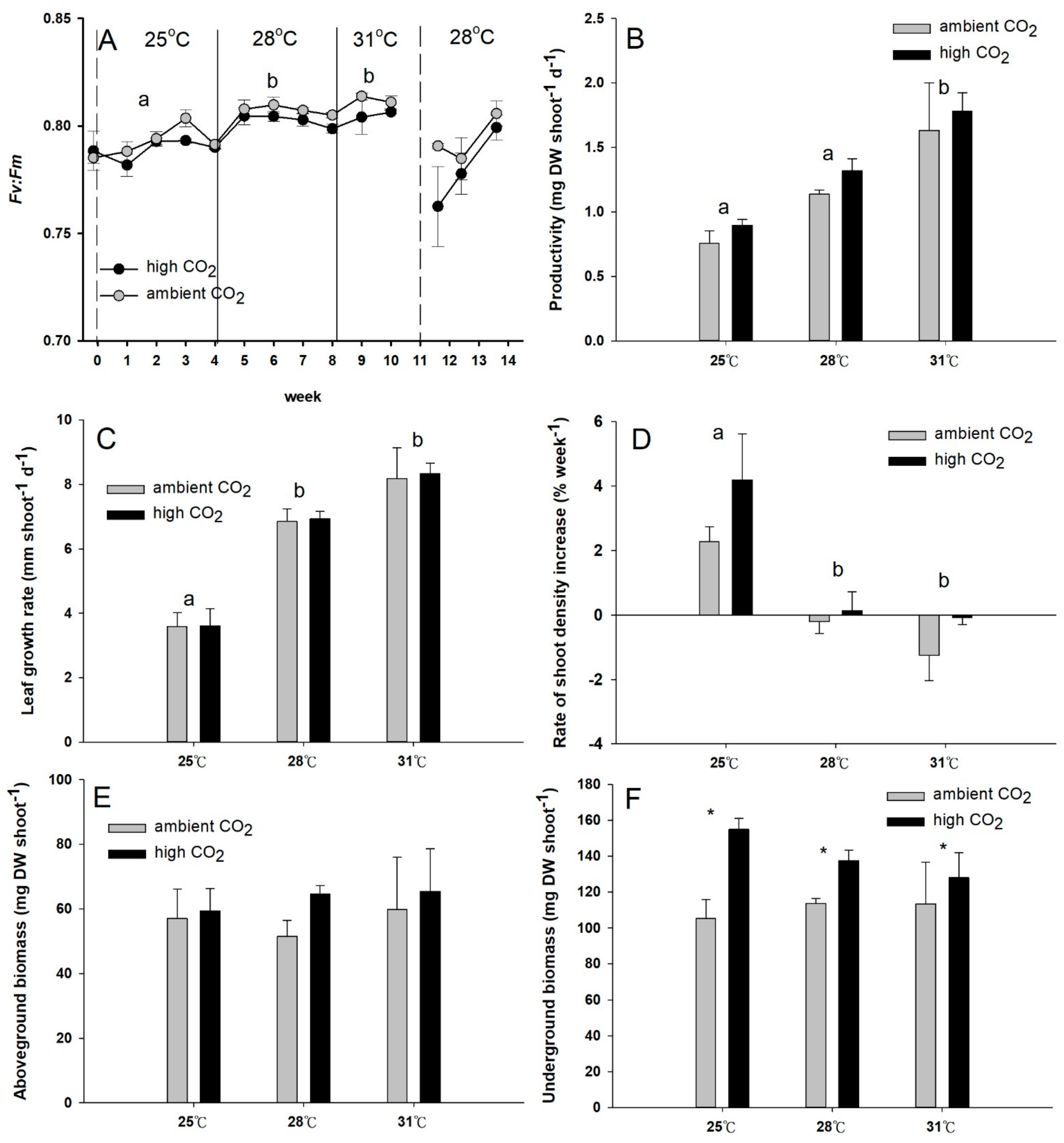
3.1. Photosynthetic Efficiency

For a thorough treatise on seawater quality analysis, please see the Supplemental Material. With respect to seagrass response variables, Fv:Fm values (Figure 2A) increased with increasing temperature for seagrass plots of both CO2 regimes (Table 1). There was no interaction of CO2 and temperature (Table 1). The Fv:Fm values dropped when the temperature decreased from 31 to 28 °C and then returned slowly to initial levels three weeks later (Figure 2A).

3.2. Productivity, Leaf Growth Rate, and Rate of Shoot Density Increase

The productivity did not differ between samples incubated at control and high CO2 levels (Figure 2B and Table 1), nor did leaf growth rate (Figure 2C and Table 1) or rate of shoot density increase (Figure 2D and Table 1). However, the productivity in both control and high-CO2 mesocosms increased as the temperature increased from 28 to 31 °C (Figure 2B and Table 1). The leaf growth rate increased with increasing temperature (Figure 2C and Table 1). In contrast, the rate of shoot density increase (Figure 2D) decreased with increasing temperature in both control and high-CO2 mesocosms (Table 1).

3.3. Aboveground and Underground Biomass

Although the aboveground biomass of T. hemprichii did not differ between control and high-CO2 mesocosms (Figure 2E), the underground biomass was higher in seagrass samples incubated at high CO2 (Figure 2F and Table 1). Temperature did not influence above- or underground biomass in either control or high-CO2 mesocosms (Figure 2E,F and Table 1), nor was the ratio of underground to aboveground biomass (U/A ratio; Table S3) affected by CO2, temperature, or their interaction (Table 1).

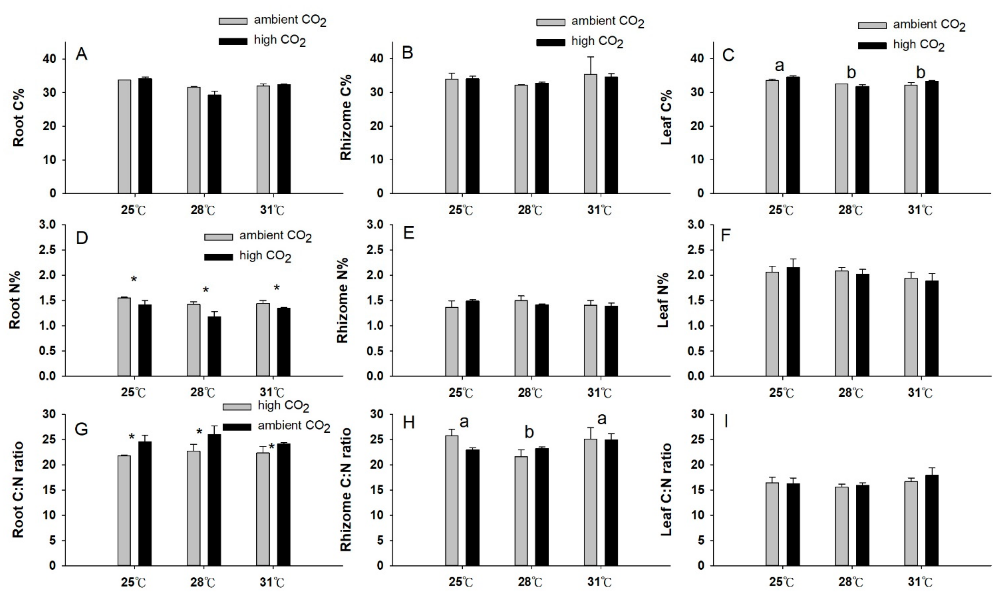
3.4. Carbon and Nitrogen Content

The carbon content of the roots, rhizomes, and leaves of T. hemprichii did not differ significantly between control and high-CO2 mesocosms (Figure 3A–C, respectively, and Table 1). However, the carbon content of the leaves decreased significantly with increasing temperature in both control and high-CO2 mesocosms (Figure 3C and Table 1); the temperature × CO2 interaction was marginally significant. The root and rhizome carbon content were not influenced by temperature (Figure 3A,B, respectively, and Table 1).
The nitrogen content of the T. hemprichii rhizomes (Figure 3E) and leaves (Figure 3F) was not affected by temperature, CO2, or their interaction (Table 1). However, the nitrogen content of the roots decreased significantly in high-CO2 mesocosms relative to the control ones (Figure 3D and Table 1). The root nitrogen content was not influenced by temperature. The rhizome (Figure 3H) and leaf (Figure 3I) C:N ratios were not influenced by OA (Table 1); however, the rhizome C:N ratios were influenced by temperature (Figure 3H and Table 1). In contrast, the root C:N ratios were higher at high CO2, though they were not influenced by temperature (Figure 3G and Table 1).

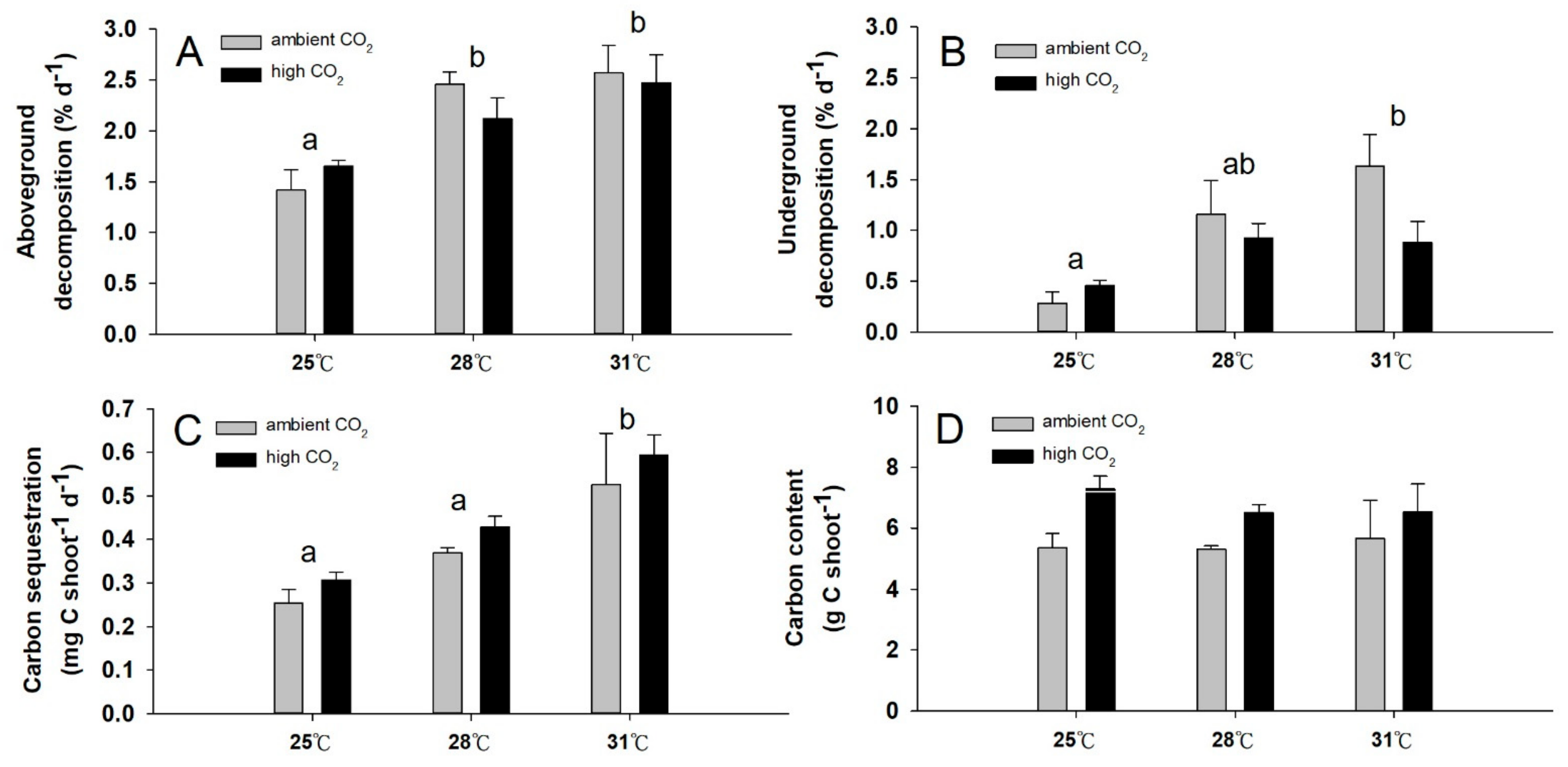
3.5. Decomposition Rate and Carbon Sequestration

Neither the decomposition rates (aboveground (Figure 4A) or underground (Figure 4B)) nor the carbon sequestration of T. hemprichii (Figure 4C) differed significantly between control and high-CO2 mesocosms (Table 1). However, all three increased with increasing temperatures. The shoot carbon content (Figure 4D) was unaffected by temperature or CO2 (Table 1).

4. Discussion

4.1. The Effects of OA

Elevated seawater CO2 is associated with increased [HCO3], and this excess bicarbonate could theoretically be used in photosynthesis. This has indeed been shown in the temperate seagrasses Zostera marina and Ruppia maritima [44], as well as in Cymodocea nodosa [45,46,47]. In our experiment, OA did not increase Fv:Fm, but instead increased underground biomass, and such enhancements might be related to this increased availability of carbon. The underground biomass of other seagrass species, such as Z. marina, Posidonia oceanica, Cymodocea serrulata, and C. nodosa, also increased under OA conditions [23,48,49,50,51]. Furthermore, Jiang et al. [52] documented increases in T. hemprichii leaf growth rate, nonstructural carbohydrates, and carbon content in underground tissues exposed to OA. It appears that at high CO2, seagrasses photosynthetically fix carbon at levels in excess of what is needed for growth and respiration; they then store the excess carbon belowground. Seagrasses cannot photosynthesize when their leaves are buried or smothered; during such high-sedimentation periods, the underground portions of the plants could support seagrass survival and even growth [53]. Having this elevated level of underground biomass could more generally aid in seagrass survival when other environmental conditions become unfavorable.
OA did not appreciably influence seagrass productivity; only root nitrogen content decreased under OA (resulting in an increase in the C:N ratios). The reason may be due to nutrient limitation or competition with other primary producers in the mesocosms, namely corals, macroalgae, and microalgae. Alexandre et al. [54] found that the leaf production of Z. noltii depends on nitrogen availability under OA. Campbell and Fourqurean [55] also found that, in situ, the nitrogen and phosphorus content of T. testudinum both decline in response to OA, but nonstructural carbohydrates increase in underground tissues. Egea et al. [25] also suggested that nutrient availability influenced C. nodosa; in their study, the photosynthetic yield improved under OA but the growth was ultimately thwarted by low nitrogen levels. Although we did not measure the growth, photosynthetic rates, or biochemical composition of other constituents of the mesocosms (e.g., corals or macroalgae), it is certainly possible that they could have competed with the seagrass for nutrients. Future mesocosm-based OA analyses should more carefully look at the physiology of multiple species, as well as the interactions among them (sensu Liu et al. [56]).

4.2. The Effects of OW

In our experiments, elevated temperature increased seagrass Fv:Fm, productivity, leaf growth rate, decomposition rate, and carbon sequestration, but decreased rate of shoot density increase and the carbon content of the leaves. Furthermore, although Fv:Fm generally rose with rising temperature, it decreased markedly during the recovery period; this could signify a delayed stressed response. Previous studies have found that OW increases the rate of seagrass respiration, decreases net photosynthetic production [57], and reduces the oxygen partial pressure within the plant; the latter can lead to sulfide uptake, which can ultimately poison the seagrass [58]. Indeed, high-temperature stress has been known to cause local extinction of seagrasses, as well as the myriad organisms that rely on them for their survival [59]. In 2015, the United States National Park Service recorded water temperatures exceeding 34 °C for more than two months in Florida Bay (https://www.nps.gov/ever/learn/nature/upload/seagrass-Dieoff_final_web_hi_res.pdf, accessed on 8 May 2020). Furthermore, DO levels were virtually 0 at night, and hydrogen sulfide levels rose; this led to a mass die-off of seagrass (over 40,000 acres).
However, the adverse effects of warming are more likely to occur in species living in areas where temperature tolerance is limited [60]. T. hemprichii is a tropical seagrass species, and it can thrive at temperatures up to 33 °C [61]. Therefore, the highest temperature employed herein, 31 °C, may not have been stress-inducing, especially given that the photosynthetic efficiency, productivity, and leaf growth rate all increased from 25 to 31 °C (though see comment above regarding the decline in Fv:Fm during the recovery period). Such an increase in photosynthetic performance would indeed be predicted to result in enhanced growth, though, in contrast, the overall plant biomass was unaffected by temperature; this may suggest that elevated temperature leads to accelerated metabolism [62] and respiration of the seagrass and co-cultured organisms.

4.3. The Effects of OA and OW

GCC has been predicted to lead to organic carbon loss in the soil [63]. Herein, the decomposition rates of the shoots both above and underground increased significantly after the temperature was raised from 25 to 28 °C. This could be due to metabolic rate increases in the small invertebrates and microbes responsible for such a decomposition. As a result, elevated temperatures may cause organic carbon sequestered in plant debris and buried in sediments to break down more rapidly through decomposition, reducing the capacity of these ecosystems to serve as carbon sinks. Furthermore, although T. hemprichii leaves significantly increased their productivity and carbon sequestration in response to elevated temperatures, short-term carbon storage was not influenced by temperature; this indicates that warming does not increase the short-term carbon sink capacity of this seagrass species. However, high CO2 levels appear to have offset the negative effects of high temperature on T. hemprichii with respect to the response variables assessed herein (i.e., decreased rate of shoot density increase and increased decomposition rate of seagrass debris).
Huang et al. [64] suggested that higher seawater temperatures allow for seagrass debris to be more effectively decomposed; this is evidently one reason why the carbon sink capacity of tropical seagrass beds is lower than that of temperate ones (review by Mazarrasa et al. [65]). Although we found that seagrass productivity and growth increased with increasing temperatures (and were unaffected by OA), the simultaneous increase in organic matter decomposition may eventually reduce the concentrations of nutrients upon which seagrasses rely over a longer-term timescale than only several months (i.e., the duration of our experiment). Regardless, as GCC will not only affect the seagrasses themselves, but also the myriad micro- and macrofauna living amidst them, it is currently premature to forecast conclusively the effects of GCC on seagrass beds in the tropical Indo-Pacific. Future studies should aim to conduct similar GCC-simulating experiments on seagrass bed mesocosms in which herbivory is also permitted; this might allow for more quantitative predictions on how GCC will affect the carbon budgets of seagrass bed ecosystems. As mentioned above, such additional studies could simultaneously attempt to induce physiological stress in the seagrass shoots through incubation at higher temperatures (perhaps 33–34 °C).

5. Conclusions

We found that, under OA conditions, seagrasses undergo increases in underground biomass and root C:N ratios alongside decreases in root nitrogen content. Elevated temperature instead increased Fv:Fm, productivity, leaf growth rate, aboveground decomposition, belowground decomposition, and carbon sequestration, but decreased the rate of shoot density increase, leaf carbon content, and rhizome C:N ratios. Under high CO2 and the highest temperature employed, this seagrass demonstrated its highest productivity, Fv:Fm, leaf growth rate, and carbon sequestration. Collectively, it appears that high CO2 levels offset the negative effects of high temperature on this seagrass species. However, elevated decomposition rates at high temperatures may ultimately reduce the future carbon sink capacity of these seagrass beds.

Supplementary Materials

The following supporting information can be downloaded at: https://www.mdpi.com/article/10.3390/jmse10060714/s1. Figure S1: A representative coral reef and seagrass mesocosm, Figure S2: The photosynthetically active radiation (PAR) at the seawater surface under each lamp of each tank, Figure S3: The seagrass bed study site, Figure S4: Abiotic conditions of the ambient (grey) and high-CO2 (black) mesocosms. Table S1: The mean values (±SE, n = 3) of the abiotic parameters in the ambient (i.e., control) and high-CO2 mesocosms under three different temperature treatments. AC = AquaController, Table S2: Nested, repeated measures ANOVA F-values for water quality parameters throughout the three-month study, Table S3: The mean values of the physiological response variables of the high and ambient (i.e., control) CO2 mesocosms at different temperatures (mean ± SE, n = 3).

Author Contributions

Conceived and designed the experiments: H.-J.L. and P.-J.L.; performed the experiments: H.-F.C. and P.-J.L.; contributed reagents/materials/analysis tools: H.-F.C., H.-J.L. and P.-J.L. wrote the paper: H.-F.C., P.-J.L. and A.B.M.; analyzed and interpreted data: H.-F.C., P.-J.L., A.B.M. and H.-J.L. All individuals are aware that they have been listed as authors and support the manuscript’s submission. All authors have read and agreed to the published version of the manuscript.

Funding

This work was funded by a research grant from the Ministry of Science and Technology (MOST) of Taiwan (MOST 103-2611-M-259-002 to P.J.-L., H.-J.L., and Pei-Jie Meng). This study was also financially supported by the “Innovation and Development Center of Sustainable Agriculture” from The Featured Areas Research Center Program within the Higher Education Sprout Project by the Ministry of Education of Taiwan to HJL. A.B.M. was funded by the MacArthur Foundation and the United States Fulbright Program.

Institutional Review Board Statement

Not applicable (though see main text for permitting information).

Informed Consent Statement

Not applicable.

Data Availability Statement

Please contact the corresponding author for all data associated with the manuscript.

Acknowledgments

We also thank Shin-Jing Ang and Teng-Yu Chen for help with data collection.

Conflicts of Interest

The authors declare no conflict of interest.

References

  1. Sabine, C.L.; Feely, R.A.; Gruber, N.; Key, R.M.; Lee, K.; Bullister, J.L.; Wanninkhof, R.; Wong, C.S.; Wallace, D.W.R.; Tilbrook, B.; et al. The oceanic sink for anthropogenic CO2. Science 2004, 305, 367–371. [Google Scholar] [CrossRef] [PubMed] [Green Version]
  2. Pörtner, H.O. Ecosystem effects of ocean acidification in times of ocean warming: A physiologist’s view. Mar. Ecol. Prog. Ser. 2008, 373, 203–217. [Google Scholar] [CrossRef] [Green Version]
  3. Van Vuuren, D.P.; Edmonds, J.; Kainuma, M.; Riahi, K.; Thomson, A.; Hibbard, K.; Hurtt, G.C.; Kram, T.; Krey, V.; Lamarque, J.F. The representative concentration pathways: An overview. Clim. Change 2011, 109, 5. [Google Scholar] [CrossRef]
  4. Stocker, T.F.; Qin, D.; Plattner, G.K.; Alexander, L.V.; Allen, S.K.; Bindoff, N.L.; Bréon, F.M.; Church, J.A.; Cubasch, U.; Emori, S.; et al. Technical Summary. In Climate Change 2013: The Physical Science Basis. Contribution of Working Group I to the Fifth Assessment Report of the Intergovernmental Panel on Climate Change; Stocker, T.F., Qin, D., Plattner, G.K., Tignor, M., Allen, S.K., Boschung, J., Nauels, A., Xia, Y., Bex, V., Midgley, P.M., Eds.; Cambridge University Press: Cambridge, UK; New York, NY, USA, 2013; pp. 33–115. [Google Scholar]
  5. Smith, S.V. Marine macrophytes as a global carbon sink. Science 1981, 211, 838–840. [Google Scholar] [CrossRef] [Green Version]
  6. Orr, J.; Pantoia, S.; Pörtner, H.O. Introduction to special section: The Ocean in a high-CO2 world. J. Geophys. Res. 2005, 110, C09S01. [Google Scholar]
  7. Nellemann, C.; Corcoran, E.; Duarte, C.M.; De Young, C.; Fonseca, L.E.; Grimsdith, G. Blue Carbon: The Role of Healthy Oceans in Binding Carbon; Center for Coastal and Ocean Mapping: Durham, NH, USA, 2010; 80p. [Google Scholar]
  8. Duarte, C.M.; Chiscano, C.L. Seagrass biomass and production: A reassessment. Aquat. Bot. 1999, 65, 159–174. [Google Scholar] [CrossRef]
  9. Milena, F.; Simon, B.; Genevieve, M.; David, M. Seagrasses as a sink for wastewater nitrogen: The case of the Adelaide metropolitan coast. Mar. Pollut. Bull. 2009, 58, 303–308. [Google Scholar]
  10. Fonseca, M.S.; Fisher, J.S. A comparison of canopy friction and sediment movement between four species of seagrass with reference to their ecology and restoration. Mar. Ecol. Prog. Ser. 1986, 29, 15–22. [Google Scholar] [CrossRef]
  11. Heck, K.L.; Wetstone, G.S. Habitat complexity and invertebrate species richness and abundance in tropical seagrass meadows. J. Biogeogr. 1977, 4, 135–142. [Google Scholar] [CrossRef]
  12. Nakamura, Y.; Horinouchi, M.; Nakai, T.; Sano, M. Food habits of fishes in a seagrass bed on a fringing coral reef at Iriomote Island, southern Japan. Ichthyol. Res. 2003, 50, 15–22. [Google Scholar] [CrossRef]
  13. Bell, J.D.; Pollard, D.A. Ecological of fish assemblage and fisheries associated with seagrasses. In Biology of Seagrasses: A Treatise on the Biology of Seagrasses with Special Reference to the Austrealian Region; Aquatic Plant Studies, 2; Larkum, A.W.D., McComb, A.J., Shepherd, S.A., Eds.; Elsevier: Amsterdam, The Netherlands, 1989; pp. 565–609. [Google Scholar]
  14. Parrish, J.D. Fish communities of interacting shallow-water habitats in tropical oceanic region. Mar. Ecol. Prog. Ser. 1989, 58, 143–160. [Google Scholar] [CrossRef]
  15. Edgar, G.J.; Shaw, C.; Watson, G.F.; Hammond, L.S. Comparisons of species richness, size-structure and production of benthos in vegetated and unvegetated habitats in Western Port, Victoria. J. Exp. Mar. Biol. Ecol. 1994, 176, 201–226. [Google Scholar] [CrossRef]
  16. Heck, K.L.; Able, K.W.; Roman, C.T.; Fahay, M.P. Composition, abundance, biomass, and production of macrofauna in a New England estuary: Comparisons among eelgrass meadows and other nursery habitats. Estuaries 1995, 18, 379–389. [Google Scholar] [CrossRef]
  17. Duffy, J.E. Biodiversity and the functioning of seagrass ecosystems. Mar. Ecol. Prog. Ser. 2006, 311, 233–250. [Google Scholar] [CrossRef] [Green Version]
  18. Orth, R.J.; Carruthers, T.J.B.; Dennison, W.C.; Duarte, C.M.; Fourqurean, J.W.; Heck, K.L.; Hughes, A.R.; Kendrick, G.A.; Kenworthy, W.J.; Olyarnik, S.; et al. A global crisis for seagrass ecosystems. BioScience 2006, 56, 987–996. [Google Scholar] [CrossRef] [Green Version]
  19. Gacia, E.; Duarte, C. Sediment retention by a Mediterranean Posidonia oceanica meadow: The balance between deposition and resuspension. Estuar. Coast. Shelf Sci. 2001, 52, 505–514. [Google Scholar] [CrossRef]
  20. Chiu, S.H.; Huang, Y.H.; Lin, H.J. Carbon budget of leaves of the tropical intertidal seagrass Thalassia hemprichii. Estuar. Coast. Shelf. Sci. 2013, 125, 27–35. [Google Scholar] [CrossRef]
  21. Laffoley, D.; Grimsditch, G.D. (Eds.) The Management of Natural Coastal Carbon Sinks; IUCN: Gland, Switzerland, 2009; 53p. [Google Scholar]
  22. Mcleod, E.; Chmura, G.L.; Bouillon, S.; Salm, R.; Björk, M.; Duarte, C.M.; Lovelock, C.E.; Schlesinger, W.H.; Silliman, B.R. A blueprint for blue carbon: Toward an improved understanding of the role of vegetated coastal habitats in sequestering CO2. Front. Ecol. Environ. 2011, 9, 552–560. [Google Scholar] [CrossRef] [Green Version]
  23. Palacios, S.L.; Zimmerman, R.C. Response of eelgrass Zostera marina to CO2 enrichment possible impacts of climate change and potential for remediation of coastal habitats. Mar. Ecol. Prog. Ser. 2007, 344, 1–13. [Google Scholar] [CrossRef]
  24. Andersson, A.J.; Mackenzie, F.T.; Gattuso, J.P. Effects of ocean acidification on benthic processes, organisms, and ecosystems. In Ocean Acidification; Gattuso, J.P., Hansson, L., Eds.; Oxford University Press: Oxford, UK, 2011; pp. 122–153. [Google Scholar]
  25. Egea, L.G.; Jiménez-Ramos, R.; Vergara, J.J.; Hernández, I.; Brun, F.G. Interactive effect of temperature, acidification and ammonium enrichment on the seagrass Cymodocea nodosa. Mar. Pollut. Bull. 2018, 134, 14–26. [Google Scholar] [CrossRef]
  26. Kroeker, K.J.; Kordas, R.L.; Crim, R.N.; Singh, G.G. Meta-analysis reveals negative yet variable effects of ocean acidification on marine organisms. Ecol. Lett. 2010, 13, 1419–1434. [Google Scholar] [CrossRef] [PubMed]
  27. Allison, A. The influence of species diversity and stress intensity on community resistance and resilience. Ecol. Monogr. 2004, 74, 117–134. [Google Scholar] [CrossRef]
  28. Mukai, H. Biogeography of the tropical seagrass in the western Pacific. Aust. J. Mar. Freshwater Res. 1993, 44, 1–17. [Google Scholar] [CrossRef]
  29. Liu, P.J.; Lin, S.M.; Fan, T.Y.; Meng, P.J.; Shao, K.T.; Lin, H.J. Rates of overgrowth by macroalgae and attack by sea anemones are greater for live coral than dead coral under conditions of nutrient enrichment. Limnol. Oceanogr. 2009, 54, 1167–1175. [Google Scholar] [CrossRef]
  30. Liu, P.J.; Hsin, M.C.; Huang, Y.H.; Fan, T.Y.; Meng, P.J.; Lu, C.C.; Lin, H.J. Nutrient enrichment coupled with sedimentation favors sea anemones over corals. PLoS ONE. 2015, 10, e0125175. [Google Scholar] [CrossRef]
  31. Vermaat, J.E.; Agawin, N.S.R.; Duarte, C.M.; Fortes, M.D.; Marbà, N.; Uri, J.S. Meadow maintenance, growth and productivity in a mixed Philippine seagrass bed. Mar. Ecol. Prog. Ser. 1995, 124, 215–225. [Google Scholar] [CrossRef]
  32. Lin, H.J.; Shao, K.T. Temporal changes in the abundance and growth of intertidal Thalassia hemprichii seagrass beds in southern Taiwan. Bot. Bull. Acad. Sin. 1998, 39, 191–198. [Google Scholar]
  33. Lewis, E.; Wallace, D. Program Developed for CO2 System Calculations; USA. 1998; 40p. Available online: https://www.osti.gov/dataexplorer/biblio/dataset/1464255 (accessed on 2 April 2022).
  34. Mehrbach, C.; Culberson, C.H.; Hawley, J.E.; Pytkowitz, R.M. Measurement of the apparent dissociation constants of carbonic acid in seawater at atmospheric pressure. Limnol. Oceanogr. 1973, 18, 897–907. [Google Scholar] [CrossRef]
  35. Dickson, A.G.; Millero, F.J. A comparison of the equilibrium constants for the dissociation of carbonic acid in seawater media. Deep Sea Res. Part A 1987, 34, 1733–1743. [Google Scholar] [CrossRef]
  36. Lee, K.-S.; Dunton, K.H. Production and carbon reserve dynamics of the seagrass Thalassia testudinum in Corpus Christi Bay, Texas, USA. Mar. Ecol. Prog. Ser. 1996, 143, 201–210. [Google Scholar] [CrossRef]
  37. Mayfield, A.B.; Chen, M.; Meng, P.J.; Lin, H.J.; Chen, C.S.; Liu, P.J. The physiological response of the reef coral Pocillopora damicornis to elevated temperature: Results from coral reef mesocosm experiments in Southern Taiwan. Mar. Environ. Res. 2013, 86, 1–11. [Google Scholar] [CrossRef] [PubMed]
  38. Pai, S.C.; Yang, C.C.; Riley, J.P. Effects of acidity and molybdate concentration on the kinetics of the formation of the phosphoantimonyl molybdenum blue complex. Anal. Chim. Acta 1990, 229, 115–120. [Google Scholar]
  39. Pai, S.C.; Riley, J.P. Determination of nitrate in the presence of nitrite in natural waters by flow injection analysis with a non-quantitative on-line cadmium reductor. Int. J. Environ. Anal. Chem. 1994, 57, 263–277. [Google Scholar] [CrossRef]
  40. Strickland, J.D.H.; Parsons, T.R. A Practical Handbook of Seawater Analysis, 2nd ed.; Fisheries Research Board of Canada Bulletin; The Alger Press Ltd.: Ottawa, ON, Canada, 1972; 328p. [Google Scholar]
  41. Short, F.T.; Duarte, C.M. Methods for the measurement of seagrass growth and production. In Global Seagrass Research Methods; Short, F.T., Coles, R.G., Eds.; Elsevier Science: Amsterdam, The Netherlands, 2001; pp. 155–182. [Google Scholar]
  42. Mateo, M.A.; Romero, J. Evaluating seagrass leaf litter decomposition: An experimental comparison between litter-bag and oxygen-uptake methods. J. Exp. Mar. Biol. Ecol. 1996, 202, 97–106. [Google Scholar] [CrossRef]
  43. Peterson, R.C.; Cummins, K.W. Leaf processing in a woodland stream. Freshw. Biol. 1974, 4, 343–368. [Google Scholar] [CrossRef]
  44. Buapet, P.; Rasmusson, L.M.; Gullström, M.; Björk, M. Photorespiration and carbon limitation determine productivity in temperate seagrasses. PLoS ONE. 2013, 8, e83804. [Google Scholar] [CrossRef] [Green Version]
  45. Invers, O.; Romero, J.; Pérez, M. Effects of pH on seagrass photosynthesis: A laboratory and field assessment. Aquat. Bot. 1997, 59, 185–194. [Google Scholar] [CrossRef]
  46. Invers, O.; Perez, M.; Romero, J. Bicarbonate utilization in seagrass photosynthesis: Role of carbonic anhydrase in Posidonia oceanica (L.) Delile and Cymodocea nodosa (Ucria) Ascherson. J. Exp. Mar. Biol. Ecol. 1999, 235, 125–133. [Google Scholar] [CrossRef]
  47. Invers, O.; Zimmerman, R.C.; Alberte, R.S.; Pérez, M.; Romero, J. Inorganic carbon sources for seagrass photosynthesis: An experimental evaluation of bicarbonate use in species inhabiting temperate waters. J. Exp. Mar. Biol. Ecol. 2001, 265, 203–217. [Google Scholar] [CrossRef]
  48. Zimmerman, R.C.; Kohrs, D.G.; Steller, D.L.; Alberte, R.S. Impacts of CO2 enrichment on productivity and light requirements of eelgrass. Plant Physiol. 1997, 115, 599–607. [Google Scholar] [CrossRef] [Green Version]
  49. Vizzini, S.; Tomasello, A.; Maida, G.D.; Pirrotta, M.; Mazzola, A.; Calvo, S. Effect of explosive shallow hydrothermal vents on δ13C and growth performance in the seagrass Posidonia oceanica. J. Ecol. 2010, 98, 1284–1291. [Google Scholar] [CrossRef]
  50. Russell, B.D.; Connell, S.D.; Uthicke, S.; Muehllehner, N.; Fabricius, K.E.; Hall-Spencer, J.M. Future seagrass beds: Can increased productivity lead to increased carbon storage? Mar. Pollut. Bull. 2013, 73, 463–469. [Google Scholar] [CrossRef] [Green Version]
  51. Apostolaki, T.E.; Vizzini, S.; Hendriks, I.E.; Olsen, Y.S. Seagrass ecosystem response to long-term high CO2 in a Mediterranean volcanic vent. Mar. Environ. Res. 2014, 99, 9–15. [Google Scholar] [CrossRef] [PubMed] [Green Version]
  52. Jiang, Z.J.; Huang, X.P.; Zhang, J.P. Effects of CO2 enrichment on photosynthesis, growth, and biochemical composition of seagrass Thalassia hemprichii (Ehrenb.) Aschers. J. Integr. Plant. Biol. 2010, 52, 904–913. [Google Scholar] [CrossRef]
  53. Ooi, J.L.S.; Kendrick, G.A.; Niel, P.V. Effects of sediment burial on tropical ruderal seagrasses are moderated by clonal integration. Cont. Shelf. Res. 2011, 31, 1945–1954. [Google Scholar] [CrossRef]
  54. Alexandre, A.; Silva, J.; Buapet, P.; Björk, M.; Santos, R. Effects of CO2 enrichment on photosynthesis, growth, and nitrogen metabolism of the seagrass Zostera noltii. Ecol. Evol. 2012, 2, 2625–2635. [Google Scholar] [CrossRef] [PubMed]
  55. Campbell, J.E.; Fourqurean, J.W. Mechanisms of bicarbonate use influence the photosynthetic carbon dioxide sensitivity of tropical seagrasses. Limnol. Oceanogr. 2013, 58, 839–848. [Google Scholar] [CrossRef]
  56. Liu, P.J.; Ang, S.J.; Mayfield, A.B.; Lin, H.J. Influence of the seagrass Thalassia hemprichii on coral reef mesocosms exposed to ocean acidification and experimentally elevated temperature. Sci. Total Environ. 2020, 700, 133464. [Google Scholar] [CrossRef]
  57. Perez, M.; Romero, J. Photosynthetic response to light and temperature of the seagrass Cymodocea nodosa and the prediction of its seasonality. Aquat. Bot. 1992, 43, 51–62. [Google Scholar] [CrossRef]
  58. Marbà, N.; Duarte, C.M. Mediterranean warming triggers seagrass (Posidonia oceanica) shoot mortality. Glob. Change. Biol. 2010, 16, 2366–2375. [Google Scholar] [CrossRef]
  59. Thomson, J.A.; Burkholder, D.A.; Heithaus, M.R.; Fourqurean, J.W.; Fraser, M.W.; Statton, J.; Kendrick, G.A. Extreme temperatures, foundation species, and abrupt ecosystem change: An example from an iconic seagrass ecosystem. Glob. Change Biol. 2015, 21, 1463–1474. [Google Scholar] [CrossRef] [PubMed]
  60. Smale, D.A.; Wernberg, T. Extreme climatic event drives range contraction of a habitat-forming species. Proc. R. Soc. B 2013, 280, 20122829. [Google Scholar] [CrossRef] [PubMed]
  61. Lee, K.S.; Park, S.R.; Kim, Y.K. Effects of irradiance, temperature, and nutrients on growth dynamics of seagrasses: A review. J. Exp. Mar. Biol. Ecol. 2007, 350, 144–175. [Google Scholar] [CrossRef]
  62. Short, F.T.; Neckles, H.A. The effects of global climate change on seagrasses. Aquat. Bot. 1999, 63, 169–196. [Google Scholar] [CrossRef]
  63. Kirschbaum, M.U.F. The temperature dependence of soil organic matter decomposition, and the effect of global warming on soil organic C storage. Soil. Biol. Biochem. 1995, 27, 753–760. [Google Scholar] [CrossRef]
  64. Huang, Y.H.; Lee, C.L.; Chung, C.Y.; Hsiao, S.C.; Lin, H.J. Carbon budgets of multispecies seagrass beds at Dongsha Island in the South China Sea. Mar. Environ. Res. 2015, 106, 92–102. [Google Scholar] [CrossRef]
  65. Mazarrasa, I.; Samper-Villarreal, J.; Serrano, O.; Lavery, P.S.; Lovelock, C.E.; Marbà, N.; Duarte, C.M.; Cortés, J.A. Habitat characteristics provide insights of carbon storage in seagrass meadows. Mar. Pollut. Bull. 2018, 134, 106–117. [Google Scholar] [CrossRef]
Figure 1. Experimental design and schematic of the CO2 regulation apparatus. T1, T2, and T4 were enriched with CO2 to a final concentration of ~1,200 ppm (A), ultimately resulting in a pH of ~7.75, while the other three mesocosms served as controls (ambient CO2; pH of ~8.2). Pure CO2 gas was bubbled into the tank through the “air refiners” (B; similar to the more common “microbubble stones”).
Jmse 10 00714 g001
Figure 2. Variation in select physiological response variables in Thalassia hemprichii exposed to ambient or high CO2 levels. (A) Fv:Fm, (B) productivity, (C) leaf growth rate, (D) rate of shoot density increase, (E) aboveground biomass, and (F) underground biomass in T. hemprichii samples incubated at either ambient (grey) or high (black) CO2. All values represent mean ± SE (n = 3), and letters (a, b) above bars in (AD) represent Tukey’s differences (p < 0.05) for the effect of temperature only; asterisks (*) in F instead denote CO2 effects at each temperature (p < 0.05).
Jmse 10 00714 g002
Figure 3. The chemical content of Thalassia hemprichii. The carbon content, nitrogen content, and carbon/nitrogen (C:N) ratios of roots (A,D,G, respectively), rhizomes (B,E,H, respectively), and leaves (C,F,I, respectively) in T. hemprichii plots incubated within ambient (grey) and high-CO2 (black) mesocosms. Values represent mean±SE (n = 3), and letters (a,b) above bars in (C,H) represent Tukey’s differences (p < 0.05) for the effect of temperature only; asterisks (*) in (D,G) instead denote within-stage CO2 effects (p < 0.05).
Jmse 10 00714 g003
Figure 4. Decomposition and carbon sequestration rates in Thalassia hemprichii. (A) The aboveground and (B) underground leaf decomposition, (C) carbon sequestration, and (D) shoot carbon content of T. hemprichii in ambient (grey) and high-CO2 (black) mesocosms. Values represent mean ± SE (n = 3), and Tukey’s differences (p < 0.05) denoted by lowercase letters (a,b) in (AC) represent temperature differences only.
Jmse 10 00714 g004
Table 1. One-way, partially nested, repeated-measures ANOVA of the effects of CO2 and experimental stage (i.e., temperature (temp.)) on seagrass response variables. For Fv:Fm, the tank was the repeated subject (n = 6 tanks), with week being the repeated measure (n = 11 analysis weeks; residual = 49); for all other response variables, the experimental stage was the repeated measure (n = 3; residual = 24). Note that “Tank (CO2)” was treated as a random factor rather than a main effect. Statistically significant values (p < 0.05) have been highlighted in bold font: * p < 0.05, ** p < 0.01, *** p < 0.001. NP = not presented.
Response VariableCO2Week(Temp.)Temp.Temp. × CO2
Degrees of freedom (df)-Fv:Fm1822
df-all other response variables1322
Source of variation Exact F statistics Figure
Fv:Fm2.963.6432.1 ***2.012A
Productivity (mg DW shoot−1 day−1)0.84 99.90 **0.092B
Leaf growth rate (mm shoot−1 day−1)0.08 24.10 *0.0022C
Rate of shoot density increase (% week−1)4.06 10.06 *0.352D
Aboveground biomass (mg DW shoot−1)0.35 0.140.682E
Underground biomass (mg DW shoot−1)14.90 * 0.121.072F
U/A ratio1.47 1.053.99NP
Root carbon percentage1.35 8.391.403A
Rhizome carbon percentage a1.04 2.230.043B
Leaf carbon percentage1.64 32.70 **10.72 *3C
Root nitrogen percentage16.30 * 2.010.433D
Rhizome nitrogen percentage0.27 0.170.463E
Leaf nitrogen percentage0.005 9.472.353F
Root C:N ratio10.25 * 0.300.203G
Rhizome C:N ratio0.16 21.60 *7.103H
Leaf C:N ratio0.14 3.671.653I
Aboveground decomposition (% d−1)2.20 28.90 *3.534A
Underground decomposition (% d−1)4.03 15.10 *3.144B
Carbon sequestration (mg C shoot−1 d−1)1.25 160.20 ***0.104C
Shoot carbon content (g C shoot−1)4.57 0.660.394D
a rank-transformed data.
Publisher’s Note: MDPI stays neutral with regard to jurisdictional claims in published maps and institutional affiliations.

