Adaptive Disturbance-Observer-Based Continuous Sliding Mode Control for Small Autonomous Underwater Vehicles in the Trans-Atlantic Geotraverse Hydrothermal Field with Trajectory Modeling Based on the Path

Abstract

Considering intense hydrothermal activities and rugged topography in a near-bottom environment of the trans-Atlantic geotraverse (TAG) hydrothermal mound, a small autonomous underwater vehicle (S-AUV) will suffer from time-varying disturbances, model uncertainties, actuator faults, and input saturations. To handle these issues, a fault-tolerant adaptive robust sliding mode control method is presented in this paper. Firstly, unknown disturbances, model uncertainties, and actuator faults of the S-AUV are synthesized into a lumped uncertain vector. Without requiring the upper bound and gradient of the uncertainties, a continuous adaptive finite-time extended state observer is designed to estimate the lumped uncertain vector. Then, an auxiliary dynamic system composed of continuous functions is introduced to deal with input saturations, thereby contributing to achieving fixed-time trajectory tracking control of S-AUVs. Based on a designed continuous fixed-time nonsingular fast sliding mode surface, the proposed continuous adaptive controller is chattering free. Simulated topography is built according to topographic data of the TAG mound, and a smooth trajectory model is constructed by cubic spline interpolation. Comprehensive simulations performed on an actual S-AUV model are given to validate the effectiveness and superiority of the presented algorithm.

1. Introduction

The deep-sea hydrothermal field is regarded as one of the most significant scientific discoveries in marine science in recent years [1,2,3]. To meet the urgent needs of hydrothermal research, the near-bottom exploration of hydrothermal fields is fast becoming a key instrument to conduct acoustic and optical data acquisition [4,5]. Considering the rugged topography and concentrated regions of hydrothermal deposits in the near-bottom environment [6,7], small autonomous underwater vehicles (S-AUVs) are applied to track the trajectory at 3 m height, identifying and observing hydrothermal deposits. Note that the battery capacity carried by S-AUVs is limited. Therefore, the combination of remotely operated vehicles (ROVs) and S-AUVs is chosen to save the battery energy of S-AUVs, that is, an ROV is applied to carry an S-AUV to sail from sea level to the vicinity of hydrothermal fields, then release the vehicle to complete exploration tasks. In active hydrothermal fields (such as the trans-Atlantic geotraverse (TAG) active mound), S-AUVs would inevitably suffer from unknown disturbances caused by the deep-sea environment and hydrothermal activities. Moreover, the highly non-linear strong coupling and uncertain characteristics of the S-AUV dynamics influence the controller design [8,9]. Consequently, all these issues make the fast and accurate trajectory tracking control of S-AUVs in hydrothermal fields a challenging and complicated task.

As one of the most efficient approaches to deal with non-linear systems under unknowns, perturbations, and external time-varying disturbances, the sliding mode control (SMC) method based on the sign function has been widely applied in trajectory tracking controls of multiple types of AUVs [9,10]. It is worth noting the fact that finite-time (FT) control methods based on sliding mode technology have drawbacks [11]. Recently, fixed-time control methods have been developed in multi-agent systems, manipulators, and unmanned surface vehicles, which makes the settling time function completely independent of the initial states of control systems. There are few results in the tracking control system of AUVs. In Ref. [12], an adaptive fixed-time trajectory tracking control strategy of an S-AUV was applied, and it could realize a fixed-time convergence of tracking errors. For a special S-AUV, a novel adaptive continuous fixed-time sliding mode controller has been presented in Ref. [13]. An interval type-2 fuzzy neural network (NN) approximator has been utilized to approximate time-varying uncertainties. However, self-learning algorithms, including adaptive NN techniques [14] and fuzzy methods [15], give rise to some drawbacks in hardware [16]. Uncertainties and disturbances have not been adequately addressed in the above control algorithms.

In order to further handle external disturbances and uncertainties, FT disturbance observers have been widely incorporated in various manners [17,18]. Compared with other FT observers, the FT observer based on a sliding mode technology has great advantages of simple structure, fast convergence, and strong robustness. However, traditional sliding mode observers may cause the chattering phenomenon due to the existence of sign functions. In this context, the FT second-order sliding mode observer based on the extended state observer (ESO) structure becomes much more attractive, since flexible frameworks can not only be developed for eliminating the chattering effect and lumped uncertainties but also observe state variables quickly. In Ref. [17], a finite-time ESO (FTESO) has been innovatively designed to estimate lumped uncertainties. For the S-AUV under unknown parameters and external disturbances, an FT sliding mode disturbance observer has been designed in Ref. [18], whereby FT stable convergence of the whole FTESO-based control system can be guaranteed.

On the other hand, actuator faults and input saturations are inevitable and widely exist in trajectory tracking systems of S-AUVs [19,20,21,22]. In practice, the output power of thrusters is limited, especially underwater thrusters. Given the special working environment of underwater thrusters, whereby the density of seawater differs from that of air by about 900 times, underwater thrusters rarely exceed 3000 rpm. Therefore, the saturation of control input must be considered for the control system of S-AUVs [23,24,25]. In Ref. [23], a robust model predictive control with input and state constraints has been designed. In a constrained workspace, an online optimal control scheme has been applied. For tracking systems of S-AUVs with input saturations, an adaptive robust SMC method [24] and a robust tracking control method [25] have been presented, respectively. A novel auxiliary dynamic system (ADS) has been introduced into control laws to handle the impact of input saturations. As another issue that must be considered, the actuator fault is the most typical actuator problem appearing in S-AUV tracking systems [26,27]. Therefore, it is optional and essential to solving the fault-tolerant control (FTC) problem of S-AUV systems under actuator faults. In the literature, faults are classified into lumped uncertainty terms for convenience of analysis and calculation. In Ref. [26], an adaptive FTC has been designed to achieve the fault reconstruction of S-AUVs, where FTESOs are applied to compensate for the effect of faults on control systems. With FT second-order sliding mode observers, an adaptive sliding mode FTC has been presented to achieve superior robustness under actuator faults [27].

In this paper, for the trajectory tracking control problem of an S-AUV in the TAG mound subject to unknown time-varying disturbances under uncertain model parameters, actuator faults, and input saturations, an adaptive fixed-time fault-tolerant method is constructed by combining the adaptive ESO, ADS, and nonsingular continuous fixed-time sliding mode (NCFTSM) surface. The three main contributions are described in the following parts:

(1)

An adaptive observer-based trajectory tracking control method is proposed. It is proved that tracking errors of S-AUVs can converge to the residual set in a fixed time.

(2)

We design an adaptive FTESO to estimate the lumped uncertainties and realize the self-adaption of observer parameters. Compared with Ref. [28], the upper bound of lumped uncertainties and its gradient need not to be known in the observer design.

(3)

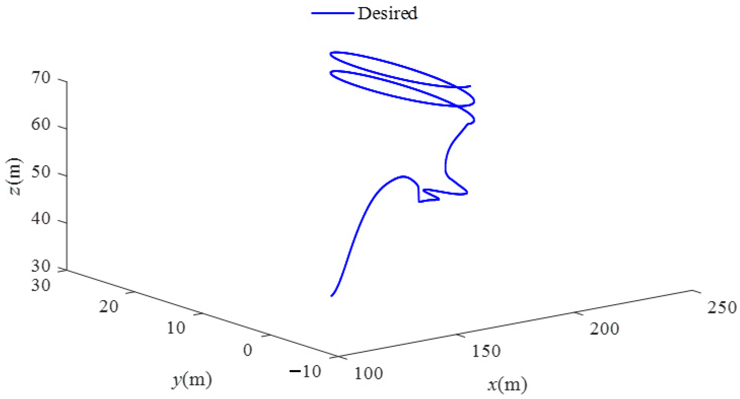
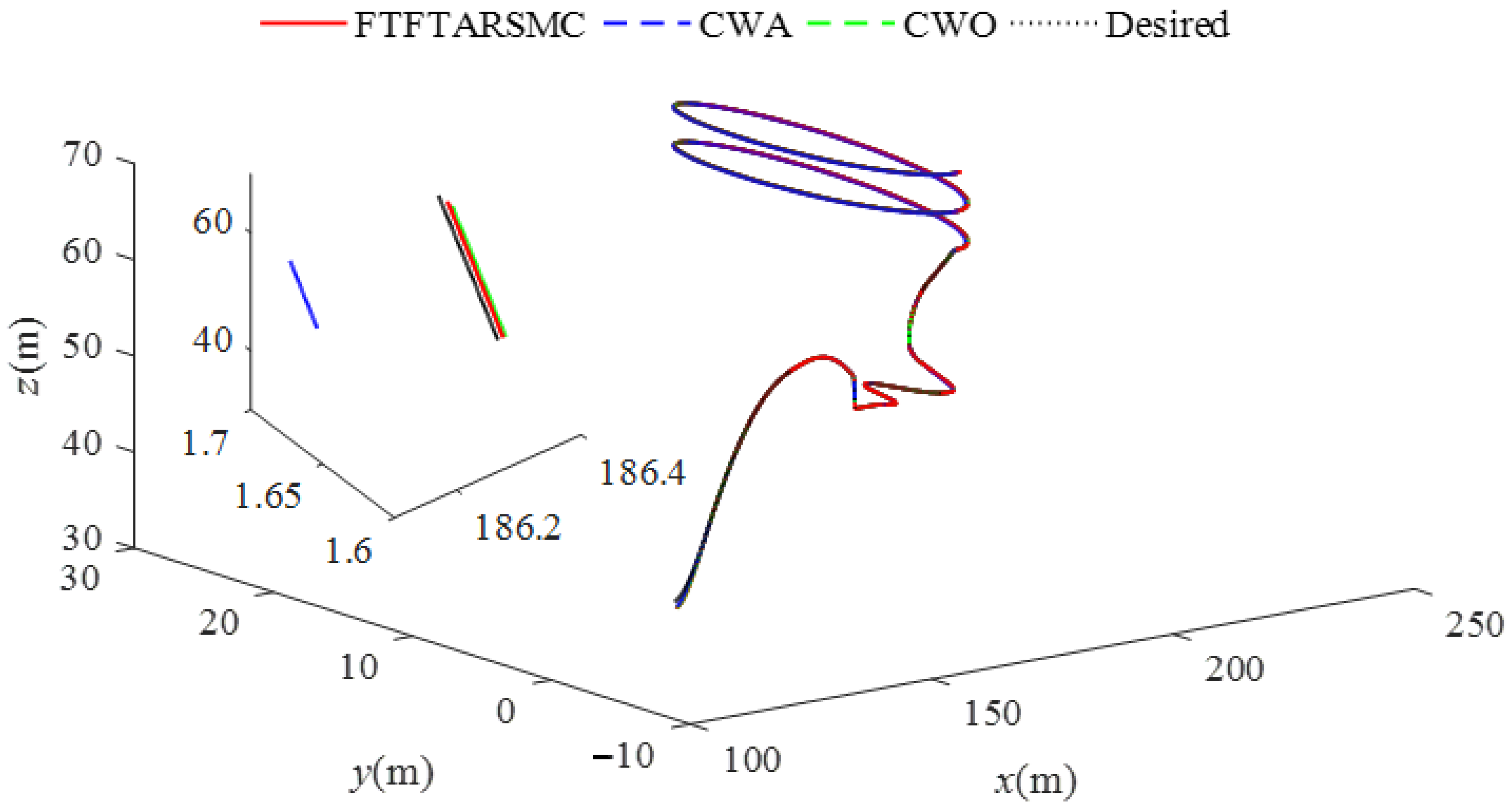
Simulated topography is built according to topographic data of the TAG hydrothermal mound. Based on the obtained path, a trajectory model is constructed by cubic spline interpolation.

Our paper is organized in the following five main sections. The tracking problem and nonlinear model of an S-AUV are given in Section 2. Section 3 gives the design of fixed-time trajectory tracking control methods and the stability analysis. Three types of control methods are compared in Section 4. Section 5 draws the conclusions.

2. Nonlinear Model and Problem Formulation

2.1. Kinematics and Dynamics of the AUV

The motion of AUVs in three-dimensional space can be described in the body-fixed motion frame (G-XYZ) and earth-fixed frame (E-X₀Y₀Z₀), as shown in Figure 1. Similarly, the general kinematics and dynamics of the vehicle in three-dimensional space are modeled by these coordinate frames. The position and attitude of AUVs in the earth-fixed frame are denoted by $\mathbf{\eta }={\left[x,y,z,\phi ,\theta ,\psi \right]}^{\mathrm{T}}$, and $\mathit{\upsilon }={\left[u,v,w,p,q,r\right]}^{\mathrm{T}}$ is used to represent the velocity of AUVs with respect to the body-fixed motion frame. Thus, the general kinematics of AUVs may be expressed as [29]

$$\dot{\mathbf{\eta }}=\mathit{J}\left(\mathit{\eta }\right)\mathit{\upsilon }$$

(1)

where $\mathit{J}\left(\mathit{\eta }\right)=\mathrm{diag}\left({\mathit{J}}_1\left(\mathit{\eta }\right),\hspace{0.17em}{\mathit{J}}_2\left(\mathit{\eta }\right)\right)\in R^{6\times 6}$ is the spatial transformation matrix between the body-fixed motion frame and the earth-fixed frame.

Assumption 1

([8]). For the transformation matrix $\mathit{J}\left(\mathit{\eta }\right)$, there exists an unknown positive constant $J_r>0$ such that $\Vert \mathit{J}\left(\eta \right)\Vert \le J_r$.

Remark 1

([8]). The pitch cannot enter the neighborhood of $\theta =\pm \pi /2$ in the actual operation of an AUV due to the existence of static restoring forces.

The dynamic equation of the AUV can be written as follows [29]:

$$\mathit{M}\dot{\mathit{\upsilon }}+\mathit{C}\left(\mathit{\upsilon }\right)\mathit{\upsilon }+\mathit{D}\left(\mathit{\upsilon }\right)\mathit{\upsilon }+\mathit{g}\left(\mathit{\eta }\right)={\mathit{\tau }}_d{}_{\eta }+{\mathit{\tau }}_v$$

(2)

where $\mathit{{\rm M}}\in R^{6\times 6}$ represents the bounded matrix of the system inertia, including the added mass, $\mathit{C}\left(\mathit{\upsilon }\right)\in R^{6\times 6}$ is the term of Coriolis-centripetal forces composed of Coriolis forces and centripetal forces, $\mathit{D}\left(\mathit{\upsilon }\right)\in R^{6\times 6}$ is the hydrodynamic damping matrix, including damping forces and damping moments, $\mathit{g}\left(\mathit{\eta }\right)\in R^{6\times 1}$ denotes the vector of restoring forces and moments caused by gravity and buoyancy, ${\mathbf{\tau }}_d{}_{\eta }={\left[{\tau }_d{{}_{\eta }}_{,1},{\tau }_d{{}_{\eta }}_{,2},{\tau }_d{{}_{\eta }}_{,3},{\tau }_d{{}_{\eta }}_{,4},{\tau }_d{{}_{\eta }}_{,5},{\tau }_d{{}_{\eta }}_{,6}\right]}^{\mathrm{T}}$ denotes unknown external disturbances of AUVs, and ${\mathit{\tau }}_v={\left[{\tau }_{v,1},{\tau }_{v,2},{\tau }_{v,3},{\tau }_{v,4},{\tau }_{v,5},{\tau }_{v,6}\right]}^{\mathrm{T}}$ denotes the actual control input vector.

With the actuator faults and saturations, in practice, the control input can be mathematically constructed as follows [30]:

$${\tau }_{vi}=\{\begin{array}{l}{\tau }_{\max i}\mathrm{sign}\left({\tau }_{ci}\right) \left|{\tau }_{ci}\right|>{\tau }_{\max i}\\ {\tau }_{ci} \left|{\tau }_{ci}\right|\le {\tau }_{\max i}\end{array} i=1,\dots ,6$$

(3)

$${\tau }_{ci}={\tau }_{ni}+b_i\left(t-t_{0i}\right)\left(\left(e_{ii}-1\right){\tau }_{ni}+{\overline{\tau }}_i\right)$$

(4)

where ${\tau }_{\max i}$ $\left(i=1,2,\dots ,6\right)$ represents the known maximum of the $i$th control input. In Equation (4), ${\tau }_{ci}$ is the control action exerted on AUVs considering the actuator fault, ${\tau }_{ni}$ is the torque command of the $i$th actuator control input from trajectory tracking controllers, ${\overline{\tau }}_i$ denotes the uncertain fault entering the AUV in an additive manner, $e_{ii}$ is an actuator fault effectiveness with $0<e_{ii}\le 1$, and $b_i\left(t-t_{0i}\right)$ describes the time profile of a fault action on the $i$th actuator that occurs at time $t_{0i}$, which can be formulated as

$$b_i\left(t-t_{0i}\right)=\{\begin{array}{l}0, t<t_{0i}\\ 1-e^{-a_i\left(t-t_{0i}\right)}, t\ge t_{0i} \end{array}$$

(5)

where $t_{0i}$ denotes the fault occurrence time, and $a_i>0$ denotes the evolution rate of unknown faults [30].

Assumption 2.

For theΔτ = [Δτ₁,…, Δτ₆]^T, it always satisfies the following condition:

$$\mathsf{\Delta }\mathbf{\tau }={\mathbf{\tau }}_v-{\mathbf{\tau }}_c$$

(6)

Assumption 3.

The additive fault of the actuator ${\overline{\tau }}_i$ in (4) is bounded by a constant $f_0>0$ satisfying $\left|{\overline{\tau }}_{}{}_i\right|<f_0$.

Taking the actuator faults and input saturations into account, the actual control input vector of AUVs can be described by

$${\mathit{\tau }}_v=\mathsf{\Delta }\mathit{\tau }+{\mathit{\tau }}_n+\mathit{B}(t-{\mathit{t}}_0)\left(\left(\mathit{E}-\mathit{I}\right){\mathit{\tau }}_n+\overline{\tau }\right)$$

(7)

where $\mathit{B}(t-{\mathit{t}}_0)=\mathrm{diag}\left(b_1\left(t-t_{01}\right),\dots ,b_6\left(t-t_{06}\right)\right)$ is a function describing the time profile of a fault, and $\mathit{E}=\mathrm{diag}\left(e_{11},\dots ,e_{66}\right)$ is the effectiveness of the actuating component.

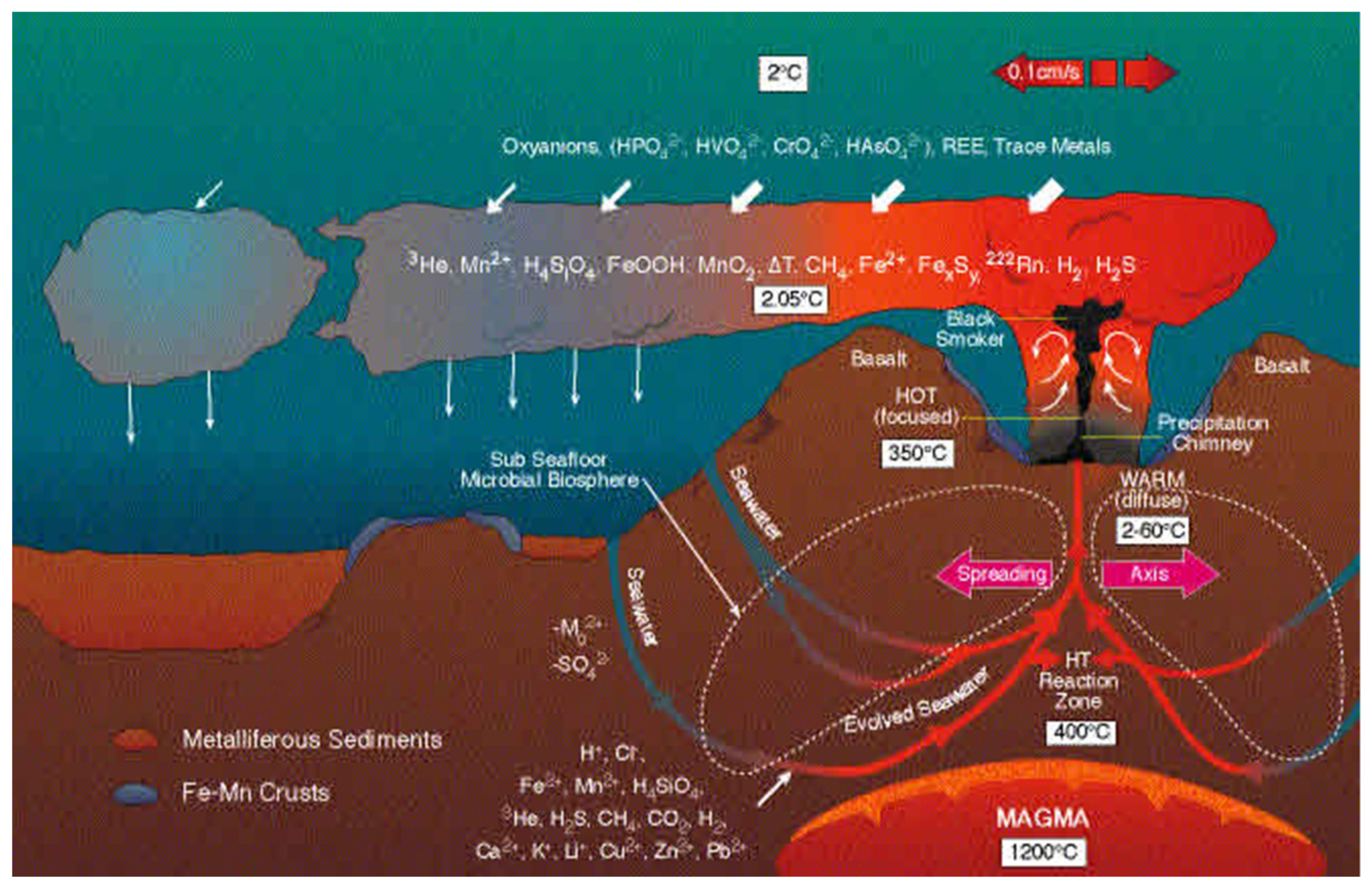
2.2. Effect of the Hydrothermal Field on AUVs

According to the characteristics of the TAG active hydrothermal mound, the effects of the hydrothermal field on S-AUVs are discussed as follows.

There are great topographic changes in the TAG active hydrothermal mound due to the intense hydrothermal activity and crustal movement. As shown in Figure 2, the active TAG mound consists of two circular terraces. There are escarpments of different heights with the slope of 25°–45° in the larger and lower terrace with 150 m in diameter. The smaller upper terrace is 90 m in diameter and has 5 m high escarpments. Fluids (360–370 °C) vent from the hydrothermal vents on the top of the 12 m high conical structure at the northwest of the terrace. Due to the influence of seabed weathering, sulfide fragments, faults, towering and collapsed hydrothermal deposits are distributed in the mound. It may cause dangerous cases if the trajectory tracking controller of S-AUVs fails to meet the requirements of high-level tracking accuracy and rapid response.

In the active hydrothermal field shown in Figure 3, the plume is produced when hydrothermal fluids are expelled from the vent. Due to the great friction, the hydrothermal fluid continues to entrain the surrounding cold seawater and rise together [32,33]. Correspondingly, the seawater near the vents will also be sucked into hydrothermal fluids below 0.6 $Z_{\max }$ ($Z_{\max }$ denotes the maximum rising height of hydrothermal plumes). When the S-AUV sails near the vent, it will be affected by the rising seawater being sucked into plumes (i.e., ${\mathit{\tau }}_d{}_f$). Meanwhile, the S-AUV also suffers from unknown disturbances from the deep-sea environment (i.e., ${\mathit{\tau }}_d{}_{\eta }$).

When the high-temperature hydrothermal activity occurs, the rising fluid continuously dissipates heat to the surrounding seawater and thereby leads to the change of the surrounding seawater in density. Distinctly, it has a great impact on the parameters $\mathit{g}\left(\mathit{\eta }\right)$ of the S-AUV model in Equation (2). Considering that the S-AUV needs to be equipped with different equipment when carrying out different tasks, the variation of loads will also cause the perturbation of the dynamic model of S-AUVs. According to the above observations, the dynamic parameters $\mathit{{\rm M}}$, $\mathit{C}\left(\mathit{\upsilon }\right)$, $\mathit{D}\left(\mathit{\upsilon }\right)$, and $\mathit{g}\left(\mathit{\eta }\right)$ have great uncertainties in practical application. Thus, the parameters of the dynamic model in Equation (2) are regarded as the sum of the nominal dynamic terms and the uncertain terms

$$\begin{gathered} \mathit{{\rm M}}=\widehat{\mathit{{\rm M}}}+\widetilde{\mathit{{\rm M}}} \\ \mathit{C}\left(\mathit{\upsilon }\right)=\widehat{\mathit{C}}\left(\mathit{\upsilon }\right)+\tilde{\mathit{C}}\left(\mathit{\upsilon }\right) \\ \mathit{D}\left(\mathit{\upsilon }\right)=\widehat{\mathit{D}}\left(\mathit{\upsilon }\right)+\tilde{\mathit{D}}\left(\mathit{\upsilon }\right) \\ \mathit{g}\left(\mathit{\eta }\right)=\widehat{\mathit{g}}\left(\mathit{\eta }\right)+\tilde{\mathit{g}}\left(\mathit{\eta }\right) \end{gathered}$$

(8)

where $\widehat{\mathit{{\rm M}}}$, $\widehat{\mathit{C}}\left(\mathit{\upsilon }\right)$, $\widehat{\mathit{D}}\left(\mathit{\upsilon }\right)$, and $\widehat{\mathit{g}}\left(\mathit{\eta }\right)$ denote the nominal dynamic terms, $\widetilde{\mathit{{\rm M}}}$, $\tilde{\mathit{C}}\left(\mathit{\upsilon }\right)$, $\tilde{\mathit{D}}\left(\mathit{\upsilon }\right)$, and $\tilde{\mathit{g}}\left(\mathit{\eta }\right)$ are the uncertain terms.

Accordingly, the S-AUV dynamic model in the active hydrothermal field can be rewritten as

$$\widehat{{\rm M}}\dot{\upsilon }+\widehat{C}\left(\mathit{\upsilon }\right)\mathit{\upsilon }+\widehat{\mathit{D}}\left(\mathit{\upsilon }\right)\mathit{\upsilon }+\widehat{g}\left(\mathit{\eta }\right)={\mathit{\tau }}_d{}_{\eta }+{\mathit{\tau }}_v+{\mathit{\tau }}_d{}_f-\mathsf{\Delta }N\left(\eta ,\mathit{\upsilon }\right)$$

(9)

where ${\mathit{\tau }}_d{}_f\in R^{6\times 1}$ represents the effect from hydrothermal plumes and is defined as unknown disturbances. $\mathsf{\Delta }N\left(\eta ,\mathit{\upsilon }\right)$ denotes the model uncertainties, which are defined as

$$\mathsf{\Delta }N\left(\eta ,\mathit{\upsilon }\right)=\widetilde{{\rm M}}\dot{\upsilon }+\tilde{C}\left(\mathit{\upsilon }\right)\mathit{\upsilon }+\tilde{\mathit{D}}\left(\mathit{\upsilon }\right)\mathit{\upsilon }+\tilde{g}\left(\mathit{\eta }\right)$$

(10)

Substituting Equation (7) into Equation (9), the complete dynamics of S-AUVs with actuator faults and saturations can be given by

$$\widehat{{\rm M}}\dot{\upsilon }+\widehat{C}\left(\mathit{\upsilon }\right)\mathit{\upsilon }+\widehat{\mathit{D}}\left(\mathit{\upsilon }\right)\mathit{\upsilon }+\widehat{g}\left(\mathit{\eta }\right)=\mathsf{\Delta }\mathit{\tau }+{\mathit{\tau }}_n+N\left(\eta ,\mathit{\upsilon }\right)$$

(11)

where the lumped system uncertainties are defined as $N\left(\eta ,\mathit{\upsilon }\right)$, which can be expressed as

$$N\left(\eta ,\mathit{\upsilon }\right)={\mathit{\tau }}_d{}_{\eta }+{\mathit{\tau }}_d{}_f-\mathsf{\Delta }N\left(\eta ,\mathit{\upsilon }\right)+\mathit{B}(t-{\mathit{t}}_0)\left(\left(\mathit{E}-\mathit{I}\right){\tau }_n+\overline{\tau }\right)$$

(12)

2.3. Problem Objective

Considering the S-AUV system described by Equations (1) and (11), the control objective is to design a fixed-time fault-tolerant adaptive robust sliding mode control (FTFTARSMC) algorithm for trajectory tracking tasks in the TAG mound. The objective of this work is met under the conditions of unknown disturbances, model uncertainties, actuator faults, and input saturations.

3. Control Design and Stability Analysis

In this section, a new adaptive continuous disturbance observer based on the ESO technique is designed, firstly to estimate lumped system uncertainties in finite time. Then, the FTFTARSMC algorithm with FT disturbance observers is developed to achieve the control object, which can guarantee that the tracking errors of S-AUVs are bounded and can converge to a small residual set within a fixed time.

3.1. Definitions and Lemmas

The following definitions and lemmas for the fixed-time controller design and the stability analysis are presented here.

Definition 1

([35]). Consider the nonlinear dynamical system

$$x=f\left(x\right),x\left(0\right)=x_0$$

(13)

where $x\in R^n$ is the system state, and $f\left(x\right):\mathsf{\Omega }\to R^n$ is continuous on an open neighborhood ${\mathsf{\Omega }}_a$ of the origin. The system (13) is said to be fixed-time stable if it is FT stable and the setting time $T\left(x_0\right)$ is uniformly bounded for $\forall x_0\in R^n$, that is, $\exists T_m>0$ such that $T\left(x_0\right)<T_m$.

Lemma 1

([35]). For the nonlinear system (13), suppose that there exists a Lyapunov function $V\left(x\right):R^n\to R$, such that the following inequality holds

$$\dot{V}\left(x\right)\le -a{V}^r\left(x\right)-b{V}^l\left(x\right)+\varsigma$$

(14)

where $a>0$, $b>0$, $r>1$, $0<l<1$, and $\varsigma$ are constants. Then, the system (13) is practical fixed-time stable. In addition, the residual set of the solution of system (13) can be given by ${\mathsf{\Omega }}_x=\left\{x|V\left(x\right)\le \min \left\{{\left[\frac{\varsigma }{a\left(1-\upsilon \right)}\right]}^{\frac{1}{r}},{\left[\frac{\varsigma }{b\left(1-\upsilon \right)}\right]}^{\frac{1}{b}}\right\}\right\}$ with $0<\upsilon <1$ and the settling time $T\left(x_0\right)$ being bounded by $T\left(x_0\right)\le \frac{1}{a\upsilon (r-1)}+\frac{1}{b\upsilon (1-l)}$.

Lemma 2

([36]). For any $\delta \in R$ and $\overline{h}\in R$, the following relationship holds

$$\delta \overline{h}\le \frac{m^q}{q}{\left|\delta \right|}^q+\frac{1}{p{m}^p}{\left|\overline{h}\right|}^p$$

(15)

where $m>0$, $q>1$ , and $p>1$ are constants satisfying $\left(q-1\right)\left(p-1\right)=1$.

Lemma 3

([37]). For any scalars ${\mathsf{\prod }}_i\in R$, $i=1,\dots ,n$, $0<r_1<1$, and $r_2>1$, the following relationships hold

$${\left({\displaystyle \sum _{i=1}^n\left|{\mathsf{\prod }}_i\right|}\right)}^{r_1}\le {\displaystyle \sum _{i=1}^n{\left|{\mathsf{\prod }}_i\right|}^{r_1}}$$

(16)

$${\left({\displaystyle \sum _{i=1}^n\left|{\mathsf{\prod }}_i\right|}\right)}^{r_2}\le n^{r_2-1}{\displaystyle \sum _{i=1}^n{\left|{\mathsf{\prod }}_i\right|}^{r_2}}$$

(17)

3.2. Finite-Time Disturbance Observer Design

To eliminate the effect of uncertainties on the trajectory tracking system of S-AUVs, the adaptive FTESO is presented. In the analysis that follows, transformation variables of state space will be introduced to facilitate the design of disturbance observers, which can be defined as

$$x_1=\mathit{\eta }·x_2=\mathit{J}\left(x_1\right)\mathit{\upsilon }$$

(18)

Then, the mathematic model (1) and (11) can be converted into

$$\begin{array}{l}{\dot{\mathit{x}}}_1={\mathit{x}}_2\\ {\dot{\mathit{x}}}_2=\mathit{J}\left({\mathit{x}}_1\right){\mathit{J}}^{-1}{\mathit{x}}_2+\mathit{J}{\widehat{\mathit{M}}}^{-1}\left({\mathit{\tau }}_n+\mathsf{\Delta }\mathit{\tau }+N\left({\mathit{x}}_1,{\mathit{x}}_2\right)-\mathit{G}\left({\mathit{x}}_1,{\mathit{x}}_2\right)\right)\end{array}$$

(19)

where $\mathit{G}\left({\mathit{x}}_1,{\mathit{x}}_2\right)=\widehat{C}\left(\mathit{\upsilon }\right)\mathit{\upsilon }+\widehat{\mathit{D}}\left(\mathit{\upsilon }\right)\mathit{\upsilon }+\widehat{\mathit{g}}\left(\mathit{\eta }\right)$.

After defining $\mathit{F}\left({\mathit{x}}_1,{\mathit{x}}_2\right)=\mathit{J}\left({\mathit{x}}_1\right){\mathit{J}}^{-1}{\mathit{x}}_2-\mathit{J}{\mathit{M}}^{-1}\mathit{G}\left({\mathit{x}}_1,{\mathit{x}}_2\right)$, we have

$$\begin{array}{l}{\dot{\mathit{x}}}_1={\mathit{x}}_2\\ {\dot{\mathit{x}}}_2=\mathit{F}\left({\mathit{x}}_1,{\mathit{x}}_2\right)+\mathit{J}{\widehat{\mathit{M}}}^{-1}\left({\mathit{\tau }}_n+\mathsf{\Delta }\mathit{\tau }\right)+\mathit{D}\end{array}$$

(20)

where $\mathit{D}=\mathit{J}{\widehat{\mathit{M}}}^{-1}N\left({\mathit{x}}_1,{\mathit{x}}_2\right)$.

Assumption 4.

The variable $\mathit{D}$including the lumped system uncertainties $N\left({\mathit{x}}_1,{\mathit{x}}_2\right)$satisfies $\Vert \mathit{D}\Vert \le H$and $\Vert \dot{\mathit{D}}\Vert \le G$. $H$and$G$exist but are not necessarily known.

The first step of the disturbance observer design is to define an auxiliary variable as

$$z_1={\mathit{x}}_2+\mathit{A}{\mathit{x}}_1$$

(21)

where $z_1:={\left[z_1,z_2,\dots ,z_6\right]}^{\mathrm{T}}$ and $A=\mathrm{diag}\left(A_1,A_2,\dots ,A_6\right)$ are positive definite matrices.

From Equation (21), the time derivative of $z_1$ is calculated as

$$\begin{array}{ll}{\dot{z}}_1={\dot{\mathit{x}}}_2+\mathit{A}{\dot{\mathit{x}}}_1& =\mathit{F}\left({\mathit{x}}_1,{\mathit{x}}_2\right)+\mathit{J}{\widehat{\mathit{M}}}^{-1}\left({\mathit{\tau }}_n+\mathsf{\Delta }\mathit{\tau }\right)+\mathit{J}{\widehat{\mathit{M}}}^{-1}\mathit{N}\left({\mathit{x}}_1,{\mathit{x}}_2\right)+\mathit{A}{\dot{\mathit{x}}}_1\\ & ={\mathit{F}}_1\left({\mathit{x}}_1,{\mathit{x}}_2\right)+\mathit{J}{\widehat{\mathit{M}}}^{-1}{\mathit{\tau }}_n+\mathit{D}\end{array}$$

(22)

where ${\mathit{F}}_1\left({\mathit{x}}_1,{\mathit{x}}_2\right)=\mathit{F}\left({\mathit{x}}_1,{\mathit{x}}_2\right)+\mathit{A}{\dot{x}}_1+\mathit{J}{\widehat{\mathit{M}}}^{-1}\mathsf{\Delta }\mathit{\tau }$.

Then, we introduce a new variable ${\mathit{z}}_2=\mathit{D}$ with considering the variable $\mathit{D}$ as an extended state, the system (22) will be expanded as follows

$$\begin{array}{l}{\dot{\mathit{z}}}_1={\mathit{F}}_1\left({\mathit{x}}_1,{\mathit{x}}_2\right)+\mathit{J}{\widehat{\mathit{M}}}^{-1}{\mathit{\tau }}_n+{\mathit{z}}_2\\ {\dot{\mathit{z}}}_2=\mathit{g}\left(t\right)\end{array}$$

(23)

where $\mathit{g}\left(t\right)$ is the first-order derivative of the variable $\mathit{D}$.

Finally, after defining the estimation error ${\mathit{e}}_1$ of auxiliary variable ${\mathit{z}}_1$ and the estimation error ${\mathit{e}}_2$ of disturbances ${\mathit{z}}_2$, the FT disturbance observer can be constructed as follows:

$$\begin{array}{l}{\mathit{e}}_1={\widehat{\mathit{z}}}_1-{\mathit{z}}_1\\ {\mathit{e}}_2={\widehat{\mathit{z}}}_2-{\mathit{z}}_2\end{array}$$

(24)

$$\begin{array}{l}{\dot{\widehat{\mathit{z}}}}_1={\mathit{F}}_1\left({\mathit{x}}_1,{\mathit{x}}_2\right)+\mathit{J}{\widehat{\mathit{M}}}^{-1}{\mathit{\tau }}_n-{\mathit{\varphi }}_1+{\widehat{\mathit{z}}}_2\\ {\dot{\widehat{\mathit{z}}}}_2=-{\mathit{\varphi }}_2\end{array}$$

(25)

where ${\widehat{\mathit{z}}}_1$ and ${\widehat{\mathit{z}}}_2$ represent the estimates of ${\mathit{z}}_1$ and ${\mathit{z}}_2$, respectively. Each element of the vectors ${\mathit{\varphi }}_1={\left[{\varphi }_{11},{\varphi }_{12},\dots ,{\varphi }_{16}\right]}^{\mathrm{T}}$ and ${\mathit{\varphi }}_2={\left[{\varphi }_{21},{\varphi }_{22},\dots ,{\varphi }_{26}\right]}^{\mathrm{T}}$ is expressed as

$$\begin{array}{l}{\varphi }_{1i}={\rho }_1{\mathrm{sig}}^{{\beta }_1}\left(e_{1i}\right)+{\rho }_2{e}_{1i}\\ {\varphi }_{2i}={\rho }_3{\mathrm{sig}}^{{\beta }_2}\left(e_{1i}\right)+\frac{1}{2}{\rho }_4{\mathrm{sig}}^{{\beta }_1}\left(e_1\right)+{\rho }_5{e}_{1i}\end{array}$$

(26)

where $i=1,2,\dots ,6$, $2/3<{\beta }_1<1$, and ${\beta }_2=2{\beta }_1-1$. The adaptive gain parameters ${\rho }_j\left(t\right)$ $\left(j=1,2,\dots ,5\right)$ are selected to satisfy

$$\begin{gathered} {\rho }_1=C_1\sqrt{R}, {\rho }_2=C_{2}R, {\rho }_3=C_{3}R, {\rho }_4=C_4{R}^{\frac{3}{2}}, {\rho }_5=C_4{R}^2 \\ \dot{R}\left(t\right)=\{\begin{array}{l}k \Vert e_1\Vert \ge {\epsilon }_0\\ 0 \Vert e_1\Vert <{\epsilon }_0\end{array} \end{gathered}$$

(27)

where the initial value $R\left(0\right)>0$, ${\epsilon }_0$ is a small positive constant, and $k>0$ is the increased rate of adaptive gains. The gain $C_k$ $\left(k=1,2,3,4\right)$ is the positive parameter and satisfies the following conditions:

$$\begin{gathered} 4{\beta }_1{}^2{C}_2{}^2{C}_3\left(C_1{}^2-C_3\right)+2{\beta }_1{C}_2{}^2{C}_3{}^2-\frac{1}{4}{C}_2{}^2{C}_3{}^2+{\beta }_1{C}_1{}^2{C}_2{}^2\left(C_1{}^2-C_1{C}_2\right)>0, \\ {C}_3=C_1{C}_2, \left(2C_3+C_1{}^2\right){\beta }_1>C_3, C_4\left(C_1-\frac{1}{2}{C}_2\right)>\left(\frac{3}{2}{C}_2-C_1\right)C_2{}^2 \end{gathered}$$

(28)

Theorem 1.

Under assumption 4, consider the expanded system (23). The FT disturbance observer described by Equations (25)–(27) can ensure that the estimation errors converge to a bounded neighborhood of the origin within a finite time$T_0$under the condition (28).

Proof of Theorem 1.

Subtracting Equations (25) and (26) into (24) yields

$$\begin{array}{l}{\dot{e}}_{1i}={\dot{\widehat{z}}}_{1i}-{\dot{z}}_{1i}=e_{2i}-{\rho }_1{\mathrm{sig}}^{{\beta }_1}\left(e_{1i}\right)-{\rho }_2{e}_{1i}\\ {\dot{e}}_{2i}={\dot{\widehat{z}}}_{2i}-{\dot{z}}_{2i}=-g{\left(t\right)}_i-{\rho }_3{\mathrm{sig}}^{{\beta }_2}\left(e_{1i}\right)-\frac{1}{2}{\rho }_4{\mathrm{sig}}^{{\beta }_1}\left(e_{1i}\right)-{\rho }_5{e}_{1i}\end{array}$$

(29)

In order to facilitate the Lyapunov analysis, the following three variables are introduced:

$${\xi }_1=\sqrt{R}·{\mathrm{sig}}^{{\beta }_1}\left(e_{1i}\right), {\xi }_2=R{e}_{1i}, {\xi }_3=e_{2i}$$

(30)

It can be known from Equation (30) that if ${\xi }_l\to 0$ $\left(l=1,2,3\right)$ in a finite time, then ${\mathit{e}}_1\to \mathbf{0}$ and ${\mathit{e}}_2\to \mathbf{0}$ in a finite time. Substituting Equation (30) into (29), we have

$${\dot{e}}_{1i}={\xi }_3-C_{1i}{\xi }_1-C_{2i}{\xi }_2$$

(31)

Taking the derivative of Equation (30) and combining it with Equation (31), we can obtain

$$\left[\begin{array}{l}{\dot{\xi }}_1\\ {\dot{\xi }}_2\\ {\dot{\xi }}_3\end{array}\right]=\left[\begin{array}{l}\frac{\dot{R}}{2R}{\xi }_1+\sqrt{R}{\beta }_1{\left|e_{1i}\right|}^{{\beta }_1-1}\left({\xi }_3-C_1{\xi }_1-C_2{\xi }_2\right)\\ \frac{\dot{R}}{R}{\xi }_2+R\left(-C_1{\xi }_1-C_2{\xi }_2+{\xi }_3\right)\\ -g{\left(t\right)}_i-C_3\sqrt{R}{\left|e_{1i}\right|}^{{\beta }_1-1}{\xi }_1-\frac{1}{2}{C}_{3}R{\xi }_1-C_{4}R{\xi }_2\end{array}\right]$$

(32)

From Equation (32), we further have

$$\dot{\xi }=\sqrt{R}{\left|e_{1i}\right|}^{{\beta }_1-1}{\mathsf{\prod }}_1\xi -R{\mathsf{\prod }}_2\xi +{\mathsf{\prod }}_3$$

(33)

where $\xi ={\left[{\xi }_1,{\xi }_2,{\xi }_3\right]}^{\mathrm{T}}$ is a column vector. The matrix ${\mathsf{\prod }}_i$ $\left(i=1,2,3\right)$ is designed as follows:

$$\begin{gathered} {\mathsf{\prod }}_1=\left[\begin{array}{ccc}{\beta }_1{C}_1& {\beta }_1{C}_2& -{\beta }_1\\ 0& 0& 0\\ C_3& 0& 0\end{array}\right], {\mathsf{\prod }}_2=\left[\begin{array}{ccc}0& 0& 0\\ C_1& C_2& -1\\ 0.5C_3& C_4& 0\end{array}\right], \\ {\mathsf{\prod }}_3=\frac{\dot{R}}{2R}\left[\begin{array}{c}{\xi }_1\\ 2{\xi }_2\\ 0\end{array}\right]-\left[\begin{array}{c}0\\ 0\\ g{\left(t\right)}_i\end{array}\right] \end{gathered}$$

(34)

Then, we need to prove the FT convergence of the matrix $\mathsf{\xi }$. The following Lyapunov function for S-AUV tracking systems is constructed as

$$V=\frac{1}{2}{\xi }^{\mathrm{T}}P\xi$$

(35)

where $P\in R^{3\times 3}$ denotes a positive definite matrix and is chosen as follows

$$P=\left[\begin{array}{ccc}4C_3+C_1{}^2& C_1{C}_2& -C_1\\ C_1{C}_2& 2C_4+C_2{}^2& -C_2\\ -C_1& -C_2& 2\end{array}\right]$$

(36)

Substituting Equation (36) into (35), $V$ can be written as

$$V=2C_3{\left|{\xi }_1\right|}^2+C_4{\left|{\xi }_2\right|}^2+\frac{1}{2}{\left|{\xi }_3\right|}^2+\frac{1}{2}{\left|C_1{\xi }_1+C_2{\xi }_2-{\xi }_3\right|}^2$$

Differentiating $V$ with respect to time and applying Equation (33) yields

$$\begin{array}{l}\dot{V}=\frac{1}{2}\left(\left({\dot{\xi }}^{\mathrm{T}}\right)P\xi +{\xi }^{\mathrm{T}}P\left(\dot{\xi }\right)\right)\\ =\frac{1}{2}({\left(\sqrt{R}{\left|e_{1i}\right|}^{{\beta }_1-1}{\mathsf{\prod }}_1\xi -R{\mathsf{\prod }}_2\xi +{\mathsf{\prod }}_3\right)}^{\mathrm{T}}P\xi \\ +{\xi }^{T}P\left(\sqrt{R}{\left|e_{1i}\right|}^{{\beta }_1-1}{\mathsf{\prod }}_1\xi -R{\mathsf{\prod }}_2\xi +{\mathsf{\prod }}_3\right))\end{array}$$

(37)

From Equation (38), we further have

$$\dot{V}=-\sqrt{R}{\left|e_{1i}\right|}^{{\beta }_1-1}{\xi }^{\mathrm{T}}{A}_1\xi -R{\xi }^{\mathrm{T}}{A}_2\xi +A_3$$

(38)

where $A_1=\left(1/2\right)\left({\mathsf{\prod }}_1{}^{\mathrm{T}}P+P{\mathsf{\prod }}_1\right)$, $A_2=\left(1/2\right)\left({\mathsf{\prod }}_2{}^{\mathrm{T}}P+P{\mathsf{\prod }}_2\right)$, and $A_3={\xi }^{\mathrm{T}}P{\mathsf{\prod }}_3$. In addition, matrices $A_1$ and $A_2$ are calculated as

$$\begin{gathered} A_1=\left[\begin{array}{ccc}\left(4C_4+C_1{}^2\right){\beta }_1{C}_1-C_1{C}_3& \left(2C_3+C_1{}^2\right){\beta }_1{C}_2-0.5C_2{C}_3& -\left(2C_3+C_1{}^2\right){\beta }_1+C_3\\ \left(2C_3+C_1{}^2\right){\beta }_1{C}_2-0.5C_2{C}_3& {\beta }_1{C}_1{C}_2{}^2& -{\beta }_1{C}_1{C}_2\\ -\left(2C_3+C_1{}^2\right){\beta }_1+C_3& -{\beta }_1{C}_1{C}_2& {\beta }_1{C}_1\end{array}\right], \\ {A}_2=\left[\begin{array}{ccc}{C}_1{}^2{C}_2-0.5C_1{C}_3& \left(0.5C_4+C_2{}^2\right)C_1-0.25C_2{C}_3& -C_1{C}_2+0.5C_3\\ \left(0.5C_4+C_2{}^2\right)C_1-0.25C_2{C}_3& C_2{C}_4+C_2{}^3& -C_2{}^2\\ -C_1{C}_2+0.5C_3& -C_2{}^2& C_1\end{array}\right] \end{gathered}$$

(39)

Defining ${\mathsf{\prod }}_{31}=\left(\dot{R}/2R\right){\left[\begin{array}{ccc}{\xi }_1& 2{\xi }_2& 0\end{array}\right]}^{\mathrm{T}}$ and ${\mathsf{\prod }}_{32}=-{\left[\begin{array}{ccc}0& 0& g{\left(t\right)}_i\end{array}\right]}^{\mathrm{T}}$, we have the following condition:

$${\mathsf{\prod }}_3={\mathsf{\prod }}_{31}+{\mathsf{\prod }}_{32}$$

(40)

Combining with Equations (39) and (41), $A_3$ can be expressed as

$$A_3={\xi }^{\mathrm{T}}P\left({\mathsf{\prod }}_{31}+{\mathsf{\prod }}_{32}\right)={\xi }^{\mathrm{T}}P{\mathsf{\prod }}_{31}+{\xi }^{\mathrm{T}}P{\mathsf{\prod }}_{32}=A_{31}+A_{32}$$

(41)

with

$$\begin{array}{c}{A}_{31}={\xi }^{T}P{\mathsf{\prod }}_{31}=\frac{\dot{R}}{2R}(\left(4C_3+C_1{}^2\right){\xi }_1{}^2+3C_1{C}_2{\xi }_1{\xi }_2\\ -C_1{\xi }_1{\xi }_2+\left(2C_4+C_2{}^2\right){\xi }_2{}^2-2C_2{\xi }_2{\xi }_3)\end{array}$$

(42)

$$A_{32}={\xi }^{\mathrm{T}}P{\mathsf{\prod }}_{32}=-g{(t)}_i\left[C_1{\xi }_1+C_2{\xi }_2-2{\xi }_3\right]$$

(43)

From the above equations, $A_{31}$ and $A_{32}$ satisfy the following conditions:

$$A_{31}\le \frac{\dot{R}}{2R}{\xi }^{\mathrm{T}}{\tilde{\mathsf{\prod }}}_{31}\xi$$

(44)

$$A_{32}\le \left|g{(t)}_i\right|\sqrt{\left(4+C_1{}^2+C_2{}^2\right)}\Vert \xi \Vert$$

(45)

with ${\tilde{\mathsf{\prod }}}_{31}=\mathrm{diag}\left({\lambda }_{{\tilde{\mathsf{\prod }}}_{31}}^1,{\lambda }_{{\tilde{\mathsf{\prod }}}_{31}}^2,{\lambda }_{{\tilde{\mathsf{\prod }}}_{31}}^3\right)$, where ${\lambda }_{{\tilde{\mathsf{\prod }}}_{31}}^1=\left(4C_3+C_1{}^2\right)+1.5C_1{C}_2+0.5C_1$, ${\lambda }_{{\tilde{\mathsf{\prod }}}_{31}}^2=\left(2C_4+C_2{}^2\right)+1.5C_1{C}_2$, and ${\lambda }_{{\tilde{\mathsf{\prod }}}_{31}}^3=0.5C_1$.

For the convenience of analysis and calculation, $\dot{V}$ satisfies the following inequality:

$$\dot{V}\le -\sqrt{R}{\left|e_{1i}\right|}^{{\beta }_1-1}{\xi }^{\mathrm{T}}{\tilde{A}}_1\xi -R{\xi }^{\mathrm{T}}{\tilde{A}}_2\xi +A_{31}+A_{32}$$

(46)

with

$${\tilde{A}}_1=\left[\begin{array}{ccc}\left(4C_3+C_1{}^2\right){\beta }_1{C}_1-C_1{C}_3& 2C_3{\beta }_1{C}_2-0.5C_2{C}_3& -\left(2C_3+C_1{}^2\right){\beta }_1+C_3\\ 2C_3{\beta }_1{C}_2-0.5C_2{C}_3& {\beta }_1{C}_1{C}_2{}^2& -{\beta }_1{C}_1{C}_2\\ -\left(2C_3+C_1{}^2\right){\beta }_1+C_3& -{\beta }_1{C}_1{C}_2& {\beta }_1{C}_1\end{array}\right]$$

(47)

$${\tilde{A}}_2=\left[\begin{array}{ccc}{C}_1{}^2{C}_2-0.5C_1{C}_3& 0& -C_1{C}_2+0.5C_3\\ 0& C_2{C}_4+C_2{}^3& -C_2{}^2\\ -C_1{C}_2+0.5C_3& -C_2{}^2& C_1\end{array}\right]$$

(48)

It can be easily verified that ${\tilde{A}}_1$ and ${\tilde{A}}_2$ are positive definite matrices satisfying the conditions (28). The following inequalities hold due to the properties of positive definite matrices

$${\lambda }_{\min }\left({\tilde{A}}_j\right){\Vert \xi \Vert }^2\le {\xi }^{\mathrm{T}}{\tilde{A}}_j\xi \le {\lambda }_{\max }\left({\tilde{A}}_j\right){\Vert \xi \Vert }^2 j=1,2$$

(49)

Similarly, for the matrix $P$ defined in Equation (36), we can obtain ${\lambda }_{\min }\left(P\right){\Vert \xi \Vert }^2\le 2V\le {\lambda }_{\max }\left(P\right){\Vert \xi \Vert }^2$. As a result, we have the following inequalities:

$$\frac{2{\lambda }_{\min }\left({\tilde{A}}_j\right)V}{{\lambda }_{\max }\left(P\right)}\le {\xi }^{\mathrm{T}}{\tilde{A}}_j\xi \le \frac{2{\lambda }_{\max }\left({\tilde{A}}_j\right)V}{{\lambda }_{\min }\left(P\right)}$$

(50)

Substituting Equations (45), (46), and (51) into (47) yields

$$\begin{array}{l}\dot{V}\le -\sqrt{R}{\left|e_{1i}\right|}^{{\beta }_1-1}\frac{2{\lambda }_{\min }\left({\tilde{A}}_1\right)V}{{\lambda }_{\max }\left(P\right)}-R\frac{2{\lambda }_{\min }\left({\tilde{A}}_2\right)V}{{\lambda }_{\max }\left(P\right)}\\ +\frac{\dot{R}}{2R}\frac{2{\lambda }_{\max }\left({\tilde{\mathsf{\prod }}}_{31}\right)V}{{\lambda }_{\min }\left(P\right)}+\left|g{(t)}_i\right|\sqrt{\left(4+C_1{}^2+C_2{}^2\right)}\Vert \xi \Vert \end{array}$$

(51)

Note that $\left|g{(t)}_i\right|\le \Vert \dot{\mathit{D}}\Vert <G$, $\sqrt{2V/{\lambda }_{\max }\left(P\right)}\le \Vert \xi \Vert \le \sqrt{2V/{\lambda }_{\min }\left(P\right)}$, and $-{\left|e_{1i}\right|}^{{\beta }_1-1}=-R^{1-{\beta }_1}{\left|{\xi }_2\right|}^{{\beta }_1-1}\le -R^{1-{\beta }_1}\left(1/{\Vert \xi \Vert }^{1-{\beta }_1}\right)$, the following inequalities for the variables $1/{\Vert \xi \Vert }^{1-{\beta }_1}$ hold

$$\frac{{\lambda }_{\min }{}^{\frac{1-{\beta }_1}{2}}\left(P\right)}{2^{\frac{1-{\beta }_1}{2}}{V}^{\frac{1-{\beta }_1}{2}}}\le \frac{1}{{\Vert \xi \Vert }^{1-{\beta }_1}}\le \frac{{\lambda }_{\max }{}^{\frac{1-{\beta }_1}{2}}\left(P\right)}{2^{\frac{1-{\beta }_1}{2}}{V}^{\frac{1-{\beta }_1}{2}}}$$

(52)

Applying Equation (53) to (52), $\dot{V}$ satisfies

$$\dot{V}\le -\left(R{\upsilon }_2-\frac{\dot{R}}{R}{\upsilon }_1\right)V-R^{\frac{3}{2}-{\beta }_1}{\upsilon }_3{V}^{\frac{1+{\beta }_1}{2}}+{\upsilon }_{4}G{V}^{\frac{1}{2}}$$

(53)

where the obtained known parameters ${\upsilon }_1=\left({\lambda }_{\max }\left({\tilde{\mathsf{\prod }}}_{31}\right)\right)/\left({\lambda }_{\min }\left(P\right)\right)$, ${\upsilon }_2=\left(2{\lambda }_{\min }\left({\tilde{\mathsf{\prod }}}_{31}\right)\right)/\left({\lambda }_{\max }\left(P\right)\right)$, ${\upsilon }_3=\left({\lambda }_{\min }\left({\tilde{A}}_1\right){\lambda }_{\min }{}^{\left(1-{\beta }_1\right)/2}\left(P\right)\right)/\left(2^{\left(1+{\beta }_1\right)/2}{\lambda }_{\max }\left(P\right)\right)$, and ${\upsilon }_4=\sqrt{2\left(4+C_1{}^2+C_2{}^2\right)/{\lambda }_{\min }\left(P\right)}$ are all constants. Since $\dot{R}=k>0$, it is easy to find that $R{\upsilon }_2-\left(\dot{R}/R\right){\upsilon }_1\ge 0$ will hold within a finite time $T_0$. After that, we have $\dot{V}\le -{\ell }_1{V}^{\left(1+{\beta }_1\right)/2}+{\ell }_2{V}^{1/2}$. According to the proof of lemma 4 in Ref. [38], the vector $\xi$ will converge with the origin within a finite time $T_0$, and $T_0\le V_0^{{}^{\left(1-{\beta }_1\right)/2}}/\left[\left(R^{\left(3/2\right)-{\beta }_1}{\upsilon }_3-\theta \right)\left(1-{\beta }_1\right)/2\right]$ with a small positive constant $\theta \in \left(0,{\ell }_1\right)$. Thus, we can obtain the result of Theorem 1. □

Remark 2.

Based on the work in Ref. [39], although greater constraints are applied to the parameters, a more detailed stability analysis is performed, and the term$\left(1/2\right){\rho }_{4i}{\mathrm{sig}}^{{\beta }_1}\left(e_{1i}\right)$is added to obtain a faster convergence rate of unknown terms. Compared with the observer in Ref. [37], the proposed observer needs not to know the upper bound of lumped uncertainties and its gradient. Therefore, it gives rise to superior performance in practical engineering.

3.3. Fixed-Time Tracking Control Design

In this subsection, the FTFTARSMC law is presented. Firstly, a fast NCFTSM manifold consisting of trajectory tracking errors is defined. Next, an ADS is introduced to deal with the input saturations. At last, we present the adaptive robust controller, which ensures that the tracking errors of S-AUVs are bounded and can converge to a small residual set $\mathsf{\Omega }$ within the fixed time.

Define the trajectory tracking errors as

$$e_3=\eta -{\mathit{\eta }}_d=x_1-x_{1d}$$

(54)

$$e_4=\dot{\eta }-{\dot{\eta }}_d={\dot{x}}_1-{\dot{x}}_{1d}$$

(55)

where $e_3={\left[e_{31},e_{32},e_{33},e_{34},e_{35},e_{36}\right]}^{\mathrm{T}}$, and ${\mathit{\eta }}_d\in R^{6\times 1}$ denotes the desired trajectory.

In order to obtain the fast fixed-time convergence performance of trajectory tracking errors $e_3$ and $e_4$, an NCFTSM manifold is constructed as

$$s=e_4+{\mathit{\beta }}_{3}F\left(e_3\right)+{\mathit{\beta }}_4{\left|e_3\right|}^{r_2}\mathrm{sign}\left(e_3\right)+2{\mathit{\beta }}_4{e}_3$$

(56)

where ${\mathit{\beta }}_3=\mathrm{diag}\left({\beta }_{31},{\beta }_{32},\dots ,{\beta }_{36}\right)$ and ${\mathit{\beta }}_4=\mathrm{diag}\left({\beta }_{41},{\beta }_{42},\dots ,{\beta }_{46}\right)$ are all positive definite design matrices. The matrix $\mathit{F}\left(e_3\right)\in R^{6\times 1}$ is designed as

$$F\left(e_{3i}\right)=\{\begin{array}{l}{\mathrm{sig}}^{r_1}\left(e_{3i}\right) if\left|e_{3i}\right|\ge {\epsilon }_1, {\overline{s}}_i=0 or {\overline{s}}_i\ne 0\\ l_1{e}_{3i}+l_2{\mathrm{sig}}^{r_0}\left(e_{3i}\right) if\left|e_{3i}\right|\le {\epsilon }_1, {\overline{s}}_i\ne 0\end{array}$$

(57)

where $\overline{s}=e_4+{\mathit{\beta }}_3{\left|e_3\right|}^{r_1}\mathrm{sign}\left(e_3\right)+{\mathit{\beta }}_4{\left|e_3\right|}^{r_2}\mathrm{sign}\left(e_3\right)+2{\mathit{\beta }}_4{e}_3$. The designed constant terms should satisfy $l_1=\left(2-r_1\right){\epsilon }_1{}^{r_1-1}$, $l_2=\left(r_1-1\right){\epsilon }_1{}^{r_1-r_0}$, $1<r_2<r_0\le 2$, $0<r_1<1$, and $1>{\epsilon }_1>0$.

Theorem 2.

Consider the trajectory tracking error systems (55) and (56). For the sliding mode manifold satisfying$s_i={\overline{s}}_i=0$, then errors $e_3$and $e_4$can converge with the residual set within a fixed time $T_1$, which can be further expressed as $T_1\le 2\times 6^{\left(r_2-1\right)/2}/\left({\lambda }_{\min }\left({\mathit{\beta }}_4\right)\left(r_2-1\right)\right)+\ln \left(\left(3{\lambda }_{\min }\left({\mathit{\beta }}_4\right)/{\lambda }_{\min }\left({\mathit{\beta }}_3\right)\right)+1\right)/\left(\left(1-r_1\right){\lambda }_{\min }\left({\mathit{\beta }}_4\right)\right)$.

Proof of Theorem 2.

If $s=\overline{s}=0$ is reached, we can have the following condition:

$$e_4=-{\mathit{\beta }}_3{\left|e_3\right|}^{r_1}\mathrm{sign}\left(e_3\right)-{\mathit{\beta }}_4{\left|e_3\right|}^{r_2}\mathrm{sign}\left(e_3\right)-2{\mathit{\beta }}_4{e}_3$$

(58)

The Lyapunov function is introduced as $V_0=0.5e_3^{\mathrm{T}}{e}_3$. Taking the time derivative of $V_0$, one can obtain

$${\dot{V}}_0=e_3^{\mathrm{T}}{\dot{e}}_3=e_3^{\mathrm{T}}\left(-{\mathit{\beta }}_3{\left|e_3\right|}^{r_1}\mathrm{sign}\left(e_3\right)-{\mathit{\beta }}_4{\left|e_3\right|}^{r_2}\mathrm{sign}\left(e_3\right)-2{\mathit{\beta }}_4{e}_3\right)$$

(59)

According to the definition ${\left|e_3\right|}^{r_1}\mathrm{sign}\left(e_3\right)$ and the parameter $r_m$ $\left(m=1,2\right)$, the following inequalities for ${\dot{V}}_0$ hold:

$$\begin{array}{l}{\dot{V}}_0\le \{\begin{array}{l}-e_3^T{\mathit{\beta }}_4{\left|e_3\right|}^{r_2}\mathrm{sign}\left(e_3\right) \Vert e_3\Vert >1\\ -e_3^T{\mathit{\beta }}_3{\left|e_3\right|}^{r_1}\mathrm{sign}\left(e_3\right)-2e_3^T{\mathit{\beta }}_4{e}_3 \Vert e_3\Vert \le 1\end{array}\\ \le \{\begin{array}{l}-{\lambda }_{\min }\left({\mathit{\beta }}_4\right){\displaystyle \sum _{i=1}^6{\left({\left|e_{3i}\right|}^2\right)}^{\frac{r_2+1}{2}} \Vert e_3\Vert >1}\\ -{\lambda }_{\min }\left({\mathit{\beta }}_3\right){\displaystyle \sum _{i=1}^6{\left({\left|e_{3i}\right|}^2\right)}^{\frac{r_1+1}{2}}-2{\lambda }_{\min }\left({\mathit{\beta }}_4\right){\displaystyle \sum _{i=1}^6{\left|e_{3i}\right|}^2 \Vert e_3\Vert \le 1}}\end{array}\end{array}$$

(60)

Based on Lemma 3, we obtain

$${\dot{V}}_0\le \{\begin{array}{l}-{\lambda }_{\min }\left({\mathit{\beta }}_4\right)6^{\frac{1-r_2}{2}}{V}_0{}^{\frac{r_2+1}{2}} \Vert e_3\Vert >1\\ -{\lambda }_{\min }\left({\mathit{\beta }}_3\right)V_0{}^{\frac{r_1+1}{2}}-2{\lambda }_{\min }\left({\mathit{\beta }}_4\right)V_0 \Vert e_3\Vert \le 1\end{array}$$

(61)

To facilitate the proof, we define a new variable $\zeta =V_0{}^{\left(1-r_1\right)/2}$. Combining with Equation (62), the time derivative of $\zeta$ is calculated as

$$\dot{\zeta }\le \{\begin{array}{l}-\frac{1-r_1}{2}{\lambda }_{\min }\left({\mathit{\beta }}_4\right)6^{\frac{1-r_2}{2}}{\zeta }^{n_1+1} \zeta >1\\ -\frac{1-r_1}{2}\left({\lambda }_{\min }\left({\mathit{\beta }}_3\right)+2{\lambda }_{\min }\left({\mathit{\beta }}_4\right)\zeta \right) \zeta \le 1\end{array}$$

(62)

with the constant $n_1=\left(r_2-1\right)/\left(1-r_1\right)$.

For $\left|\zeta \right|\ge 1$, by integrating and solving the differential Equation (63), one obtains

$${\displaystyle {\int }_0^{t_0}dt={\displaystyle {\int }_1^{+\infty }\frac{2}{1-r_1}\frac{1}{{\lambda }_{\min }\left({\mathit{\beta }}_4\right)6^{\left(1-r_2\right)/2}{\zeta }^{n_1+1}}d}}\zeta$$

(63)

Further, we have

$$t_0\le \frac{2}{1-r_1}{6}^{\left(r_2-1\right)/2}{\displaystyle {\int }_1^{+\infty }\frac{1}{{\lambda }_{\min }\left({\mathit{\beta }}_4\right){\zeta }^{1+n_1}}d\zeta }$$

(64)

Subsequently, the convergence time for $\left|\zeta \right|\ge 1$ is calculated as

$$t_0\le \frac{2·6^{\left(r_2-1\right)/2}}{{\lambda }_{\min }\left({\mathit{\beta }}_4\right)\left(r_2-1\right)}$$

(65)

For $\left|\zeta \right|\le 1$, by integrating and solving the differential Equation (63), we obtain

$${\displaystyle {\int }_0^{t_1}dt=-{\displaystyle {\int }_1^0\frac{2}{1-r_1}\frac{1}{{\lambda }_{\min }\left({\mathit{\beta }}_3\right)+2{\lambda }_{\min }\left({\mathit{\beta }}_4\right)\zeta }d}}\zeta$$

(66)

Next, the convergence time for $\left|\zeta \right|\le 1$ is calculated as

$$t_1\le \frac{1}{\left(1-r_1\right){\lambda }_{\min }\left({\mathit{\beta }}_4\right)}\ln \left(\frac{2{\lambda }_{\min }\left({\mathit{\beta }}_4\right)}{{\lambda }_{\min }\left({\mathit{\beta }}_3\right)}+1\right)$$

(67)

Thus, the total convergence time $T_1$ is estimated as

$$T_1\le \frac{2·6^{\left(r_2-1\right)/2}}{{\lambda }_{\min }\left({\mathit{\beta }}_4\right)\left(r_2-1\right)}+\frac{1}{\left(1-r_1\right){\lambda }_{\min }\left({\mathit{\beta }}_4\right)}\ln \left(\frac{2{\lambda }_{\min }\left({\mathit{\beta }}_4\right)}{{\lambda }_{\min }\left({\mathit{\beta }}_3\right)}+1\right)$$

(68)

The proof is finished. □

Remark 3.

Considering the NFSM surface in Ref [38], the terms$2{\mathit{\beta }}_4{e}_3$and ${\mathit{\beta }}_4{\left|e_3\right|}^{r_2}\mathrm{sign}\left(e_3\right)$are applied to improve the designed NCFTSM surface. After that, it guarantees that faster fixed-time convergence performance is realized in the region near and far away from the origin.

Remark 4.

In order to further improve the convergence rate and reliability,$r_2$is replaced by the term ${\kappa }_{1i}=0.5\left(r_2+1\right)+0.5\left(r_2-1\right)\mathrm{sign}\left(\left|e_{3i}\right|-1\right)$. Then, Equation (57) is equivalent to the following form:

$$s_i=\{\begin{array}{l}{e}_4+{\beta }_{3i}si{g}^{r_1}\left(e_{3i}\right)+{\beta }_{4i}{\left|e_{3i}\right|}^{r_2}sign\left(e_{3i}\right)+2{\beta }_{4i}{e}_{3i} if\left|e_{3i}\right|>1, {\overline{s}}_i=0 or {\overline{s}}_i\ne 0\\ e_4+{\beta }_{3i}si{g}^{r_1}\left(e_{3i}\right)+{\mathit{\beta }}_4{e}_{3i}+2{\beta }_{4i}{e}_{3i} if{\epsilon }_1<\left|e_{3i}\right|\le 1, {\overline{s}}_i=0 or {\overline{s}}_i\ne 0\\ e_4+{\beta }_{3i}\left(l_1{e}_{3i}+l_{2}si{g}^{r_0}\left(e_{3i}\right)\right)+{\beta }_{4i}{e}_{3i}+2{\beta }_{4i}{e}_{3i} if\left|e_{3i}\right|\le {\epsilon }_1,{\overline{s}}_i\ne 0\end{array}$$

(69)

Although the above- mentioned one has the advantage in convergence rate, its control law tends to be discontinuous. For that matter, it will give rise to the chattering problem. In the TAG mound, the accuracy of controllers will be inevitably affected if the control algorithm with chattering is applied to the tracking task of S-AUVs.

In order to handle input saturations, an ADS is introduced as follows [40]:

$$\dot{\xi }=-k_1{\xi }^{{\lambda }_1}-k_2{\xi }^{{\lambda }_2}-h\left(\xi \right)+\mathsf{\Delta }\tau$$

(70)

where $\xi ={\left[{\xi }_1,{\xi }_2,\dots ,{\xi }_6\right]}^{\mathrm{T}}$ denotes the state of the auxiliary system, $k_1=\mathrm{diag}\left(k_{11},k_{12},\dots ,k_{16}\right)$ and $k_2=\mathrm{diag}\left(k_{21},k_{22},\dots ,k_{26}\right)$ are all positive definite matrices. The design parameters ${\lambda }_1>1$ and $0<{\lambda }_2<1$ are constants. The matrix $h\left(\xi \right)$ is designed as

$$h\left(\xi \right)=\{\begin{array}{l}\mathbf{0} \Vert \xi \Vert <{\mu }_1\\ \frac{{\displaystyle \sum _{i=1}^6\left|{\left(s^{\mathrm{T}}\mathit{J}{\widehat{\mathit{M}}}^{-1}\right)}_i\mathsf{\Delta }{\tau }_i\right|+\varpi {\Vert \mathsf{\Delta }\tau \Vert }^{{\lambda }_2+1}}}{{\Vert \xi \Vert }^2}\xi \widehat{h}\left(\xi \right) {\mu }_1\le \Vert \xi \Vert \le {\mu }_2\\ \frac{{\displaystyle \sum _{i=1}^6\left|{\left(s^{\mathrm{T}}\mathit{J}{\widehat{\mathit{M}}}^{-1}\right)}_i\mathsf{\Delta }{\tau }_i\right|+\varpi {\Vert \mathsf{\Delta }\tau \Vert }^{{\lambda }_2+1}}}{{\Vert \xi \Vert }^2}\xi \Vert \xi \Vert >{\mu }_2\end{array}$$

(71)

where $\widehat{h}\left(\xi \right)=0.5-0.5\sin \left(L\left(\xi \right)\right)$ and $L\left(\xi \right)=\left(-\pi /2\right)\left(2\Vert \xi \Vert -{\mu }_1-{\mu }_2\right)/\left({\mu }_2-{\mu }_1\right)$. The constants $\varpi$, ${\mu }_1$, and ${\mu }_2$ respectively, satisfy $\varpi >1/\left({\lambda }_2+1\right)$ and $0<{\mu }_1<{\mu }_2$.

Based on the sliding mode manifold (57), ADS (70), and adaptive FTESO (25), we propose an FTFTARSMC algorithm for tracking errors (55) and (56) of S-AUVs as

$${\mathit{\tau }}_n=\widehat{\mathit{M}}{\mathit{J}}^{-1}\left({\mathit{\tau }}_1-{\mathit{\tau }}_2\right)+{\mathit{\tau }}_3$$

(72)

$$\begin{array}{l}{\mathit{\tau }}_1=-\mathit{F}\left(x_1,x_2\right)-{\mathit{\beta }}_3\dot{\mathit{F}}\left(e_3\right)-r_2{\mathit{\beta }}_4{\left|e_3\right|}^{r_2-1}{\dot{e}}_3-2{\mathit{\beta }}_4{\dot{e}}_3+{\ddot{x}}_{1d}\\ -k_3{s}^{{\lambda }_1}-k_4{s}^{{\lambda }_2}+k_5\xi \end{array}$$

(73)

$${\mathit{\tau }}_2={\widehat{\mathit{z}}}_2$$

(74)

$${\mathit{\tau }}_3=\{\begin{array}{l}\mathbf{0} \Vert s\Vert \le {\epsilon }_2\\ -\widehat{a}\frac{\widehat{\mathit{M}}{\mathit{J}}^{-1}s}{\Vert s\Vert }+k_A\widehat{a}\frac{\widehat{\mathit{M}}{\mathit{J}}^{-1}s}{\Vert s\Vert }+\widehat{a}\frac{\widehat{\mathit{M}}{\mathit{J}}^{-1}s}{{\Vert s\Vert }^2} \Vert s\Vert >{\epsilon }_2\end{array}$$

(75)

$$\dot{\widehat{a}}=k_A\Vert s\Vert$$

(76)

where the matrix $k_i=\mathrm{diag}\left(k_{i1},k_{i2},\dots ,k_{i6}\right)$ $\left(i=3,4,5\right)$ is positive definite, ${\epsilon }_2$ denotes a small positive constant, and $k_A>1$. With $\widehat{a}\left(0\right)>0$, $\widehat{a}$ is the estimate of $a$ and will be updated by the adaptive law (76). According to Lemma 1 of Ref [41], the gain $\widehat{a}$ is bounded, i.e., there exists a positive constant $a^{\ast }$ satisfying $a^{\ast }\ge \widehat{a}$.

In the following, the proof of the FTFTARSMC algorithm is given in Theorem 3.

Theorem 3.

Considering the S-AUV model based on Equations (1) and (11) subject to unknown disturbances, model uncertainties, actuator faults, and input saturations under Assumptions 1–5, if the conditions${\lambda }_{\min }\left(k_4\right)>{\left({\lambda }_{\max }\left(k_5\right)\right)}^{{\lambda }_2+1}/\left({\lambda }_2+1\right)$,${\lambda }_{\min }\left(k_2\right)>1/\left({\lambda }_2+1\right)$, and${\lambda }_{\min }\left(k_3\right)>6^{\left({\lambda }_1-1\right)/2}\left({\left({\lambda }_{\max }\left(k_5\right)\right)}^{{\lambda }_1+1}+1\right)/\left({\lambda }_1+1\right)$are satisfied, the proposed controller (72)–(75) with the adaptive law (76), ADS (70), adaptive FTESO (25), and NCFTSM manifold (57) can guarantee that the tracking errors (55) and (56) of S-AUVs are bounded and can converge to a residual set${\mathsf{\Omega }}_E$within a fixed time$T_2$.

Proof of Theorem 3.

Define the error $\tilde{a}=a^{\ast }-\widehat{a}$ and consider the following Lyapunov function

$$V_1=\frac{1}{2}{s}^{\mathrm{T}}s+\frac{1}{2}{\xi }^{\mathrm{T}}\xi +\frac{1}{2}{\tilde{a}}^2$$

(77)

Taking the time derivative of $V_1$ results in

$$\begin{array}{l}{\dot{V}}_1\le s^{\mathrm{T}}\left(-{\widehat{\mathit{z}}}_2+\mathit{J}{\widehat{\mathit{M}}}^{-1}N\left(x_1,x_2\right)\right)+s^{\mathrm{T}}\mathit{J}{\widehat{\mathit{M}}}^{-1}\mathsf{\Delta }\mathit{\tau }-{\lambda }_{\min }\left(k_3\right)6^{\frac{1-{\lambda }_1}{2}}{\left(s^{\mathrm{T}}s\right)}^{\frac{{\lambda }_1+1}{2}}\\ -{\lambda }_{\min }\left(k_4\right){\left(s^{\mathrm{T}}s\right)}^{\frac{{\lambda }_2+1}{2}}+{\lambda }_{\max }\left(k_5\right)s^{\mathrm{T}}\xi -{\lambda }_{\min }\left(k_1\right)6^{\frac{1-{\lambda }_1}{2}}{\left({\xi }^{\mathrm{T}}\xi \right)}^{\frac{{\lambda }_1+1}{2}}+\widehat{a}-{\xi }^{\mathrm{T}}h\left(\xi \right)\\ -{\lambda }_{\min }\left(k_2\right){\left({\xi }^{\mathrm{T}}\xi \right)}^{\frac{{\lambda }_2+1}{2}}-\frac{1}{h_1\left(1+{\lambda }_2\right)}\Vert s\Vert {\left(\tilde{a}\tilde{a}\right)}^{\frac{1+{\lambda }_2}{2}}-\frac{1}{h_2\left(1+{\lambda }_1\right)}\Vert s\Vert {\left(\tilde{a}\tilde{a}\right)}^{\frac{1+{\lambda }_1}{2}}+{\xi }^{\mathrm{T}}\mathsf{\Delta }\tau \end{array}$$

(78)

According to the characteristics of the ADS, Equations (70) and (71), (78) can be arranged as

$${\dot{V}}_1\le -a{V}_1{}^{\left(1+{\lambda }_1\right)/2}-b{V}_1{}^{\left(1+{\lambda }_2\right)/2}+\chi$$

(79)

where $a=\min \left\{a_1,a_2,a_3\right\}$, $b=\min \left\{b_1,b_2,b_3\right\}$, and $\chi =\max \left\{{\chi }_1,{\chi }_2,{\chi }_3\right\}$. The value of the matrix $\chi$ is not required to be known; it is only used for theoretical analysis.

According to Lemma 1, it is known that the S-AUV trajectory tracking control system in hydrothermal fields can realize practical fixed-time stability. From Equation (77), $\mathit{E}={\left[s^{\mathrm{T}},{\xi }^{\mathrm{T}},\tilde{a}\right]}^{\mathrm{T}}={\left[E_1{}^{\mathrm{T}},\tilde{a}\right]}^{\mathrm{T}}$ settles within the residual set

$${\mathsf{\Omega }}_E=\left\{E|V\left(E\right)\le \min \left\{{\left[\chi /\left(a\left(1-\delta \right)\right)\right]}^{2/\left({\lambda }_1+1\right)},{\left[\chi /\left(b\left(1-\delta \right)\right)\right]}^{2/\left({\lambda }_2+1\right)}\right\}\right\}$$

(80)

with $0<\delta <1$, the fixed time $T_2$ is expressed by $T_2\le 2/\left(a\delta \left({\lambda }_1-1\right)\right)+2/\left(b\delta \left(1-{\lambda }_2\right)\right)$. Further, according to Equation (79), it is worth noting that $s$, $\xi$, and $\tilde{a}$ in Equation (77) will converge to ${\mathsf{\Omega }}_E$ and be stabilized in ${\mathsf{\Omega }}_E$ if the initial variables are designed as $E_1={\left[s^{\mathrm{T}}\left(0\right),{\xi }^{\mathrm{T}}\left(0\right)\right]}^{\mathrm{T}}\in {\mathsf{\Omega }}_{E_1}$ with ${\mathsf{\Omega }}_{E_1}$ being a compact set and $\tilde{a}\left(0\right)\in {\mathsf{\Omega }}_{\tilde{a}}$. Thus, it is concluded that the S-AUV trajectory tracking control system in hydrothermal fields is semi-globally uniformly ultimately bounded. For the detailed derivation processes of (77) and (78), please refer to Appendix A. □

Remark 5.

Compared with Refs [42,43], the main improvements of the proposed trajectory tracking algorithm include: (1) Based on the analysis of the hydrothermal environment, the S-AUV control algorithm is modified with considering unknown disturbances, parameter perturbations, input saturations, and actuator faults; (2) A multi-parameter adaptive FTESO is constructed without knowing the upper bound of the lumped uncertainties and its gradient.

Remark 6.

Due to the finite-time convergent observer errors, $-{\widehat{\mathit{z}}}_2+\mathit{J}{\widehat{\mathit{M}}}^{-1}N\left(x_1,x_2\right)$may not converge to zero at $T_2$, and$s^{\mathrm{T}}\left(\mathit{J}{\widehat{\mathit{M}}}^{-1}N\left(x_1,x_2\right)-{\widehat{\mathit{z}}}_2\right)\le \kappa$holds with $\kappa \ge 0$being a positive constant. The constant $\kappa$only affects the parameter $\chi$in Equation (79). When $\chi$is large, the tracking errors may increase and lead to loss of control accuracy. The complex TAG mound and the poor performance of the forward-looking obstacle avoidance sonar at 3 m height make the fixed-time convergence ability of S-AUV tracking systems a top priority. Actually, the control performance is accepted based on the simulation results.

4. Topography Building and Trajectory Modeling

In this section, we will build the TAG active hydrothermal mound to construct the actual rugged topography in the simulink. According to the chosen path points, the desired trajectory is modeled by cubic spline interpolation.

The topography in simulations is built based on topographic data of the TAG hydrothermal mound [44,45], as shown in Figure 4. According to task requirements, the S-AUV starts from the release point, sails along the trajectory at 3 m height, passes through dense areas of hydrothermal deposits, and takes circular observations for the large active hydrothermal vents at the northwest of mound, as shown in Figure 5.

To construct a three-dimensional trajectory from the starting point $P_1$ to the final point $P_f$ in the time interval of $\left[T_1,T_f\right]$, points on the path are collected according to the path characteristics at first. Then, the whole trajectory is divided into an approaching part and an encircling part. In addition, appropriate boundary conditions are derived to guarantee the continuity of velocities. Next, cubic spline interpolation based on collected points is applied to construct the approaching trajectory to ensure that the interpolated trajectory is as close to the corresponding path as possible.

The approaching trajectory describes the spatial curve of S-AUVs from the starting point $P_1$ to the point near the vent $P_{38}$ in $\left[T_1,T_{38}\right]$. To create the approaching trajectory, 38 accuracy points on this path are considered as

$$P_j=\left(X_j,Y_j,Z_j\right)@T_j\left(j=1,2,\dots ,38\right)$$

(81)

where $T_j$ is the time instant at which the S-AUV plans to point $P_j$. Based on cubic spline interpolation methods, the mathematical models $X_j$, $Y_j$, and $Z_j$ with respect to time are constructed, and boundary conditions are guaranteed at the point $\left(X_{38},Y_{38},Z_{38}\right)$. Thus, the approaching trajectory can be defined as follows:

$$\begin{array}{l}{x}_{1d}=\mathrm{spline}\left(X,T,t_1\right)\\ y_{1d}=\mathrm{spline}\left(Y,X,x_{1d}\right)\\ z_{1d}=\mathrm{spline}\left(Z,X,x_{1d}\right)\end{array}$$

(82)

where $X=\left[X_1\dots X_{38}\right]\in R^{1\times 38}$, $Y=\left[Y_1\dots Y_{38}\right]\in R^{1\times 38}$, $Z=\left[Z_1\dots Z_{38}\right]\in R^{1\times 38}$, and $T_a=\left[T_1\dots T_{38}\right]\in R^{1\times 38}$ are constant vectors. $t_1$ denotes the total time of the approaching trajectory. According to cubic spline interpolation, $x_{1d}$, $y_{1d}$, and $z_{1d}$ in the approaching trajectory will be composed of 37 cubic polynomials for 38 points in $\left[T_1,T_{38}\right]$ and can be written as follows:

$$\{\begin{array}{l}{x}_{1d}(i,1)=x_{1d}.\mathrm{coefs}\left(i,1\right){\left(t-x_{1d}.\mathrm{breaks}\left(i\right)\right)}^3\\ +x_{1d}.\mathrm{coefs}\left(i,2\right){\left(t-x_{1d}.\mathrm{breaks}\left(i\right)\right)}^2 \\ +x_{1d}.\mathrm{coefs}\left(i,3\right)\left(t-x_{1d}.\mathrm{breaks}\left(i\right)\right)+x_{1d}.\mathrm{coefs}\left(i,4\right)\\ y_{1d}(i,1)=y_{1d}.\mathrm{coefs}\left(i,1\right){\left(x_{1d}\left(i,1\right)-y_{1d}.\mathrm{breaks}\left(i\right)\right)}^3\\ +y_{1d}.\mathrm{coefs}\left(i,2\right){\left(x_{1d}\left(i,1\right)-y_{1d}.\mathrm{breaks}\left(i\right)\right)}^2 if T_i\le t\le T_{i+1}\\ +y_{1d}.\mathrm{coefs}\left(i,3\right)\left(x_{1d}\left(i,1\right)-y_{1d}.\mathrm{breaks}\left(i\right)\right)+y_{1d}.\mathrm{coefs}\left(i,4\right)\\ z_{1d}(i,1)=z_{1d}.\mathrm{coefs}\left(i,1\right){\left(x_{1d}\left(i,1\right)-z_{1d}.\mathrm{breaks}\left(i\right)\right)}^3\\ +z_{1d}.\mathrm{coefs}\left(i,2\right){\left(x_{1d}\left(i,1\right)-z_{1d}.\mathrm{breaks}\left(i\right)\right)}^2 \\ +z_{1d}.\mathrm{coefs}\left(i,3\right)\left(x_{1d}\left(i,1\right)-z_{1d}.\mathrm{breaks}\left(i\right)\right)+z_{1d}.\mathrm{coefs}\left(i,4\right)\end{array}$$

(83)

where $i=1,2,\dots ,37$, $x_{1d}.\mathrm{coefs}\in R^{37\times 4}$, $y_{1d}.\mathrm{coefs}\in R^{37\times 4}$, and $z_{1d}.\mathrm{coefs}\in R^{37\times 4}$ are the polynomial coefficients obtained by applying the cubic spline interpolation. $x_{1d}.\mathrm{breaks}\in R^{1\times 38}$, $y_{1d}.\mathrm{breaks}\in R^{1\times 38}$, and $z_{1d}.\mathrm{breaks}\in R^{1\times 38}$ represent the known interpolated points along the curve.

For the attitude in the approaching trajectory, we choose $rol{l}_{1d}=0\mathrm{rad}$ and $pitc{h}_{1d}=0\mathrm{rad}$ based on task requirements. Similar to $x_{1d}$, $ya{w}_{1d}$ can be designed as follows:

$$ya{w}_{1d}=\mathrm{spline}\left(Yaw,T,t_1\right)$$

(84)

$$\{\begin{array}{l}rol{l}_{1d}(i,1)=0\\ pitc{h}_{1d}(i,1)=0\\ ya{w}_{1d}(i,1)=ya{w}_{1d}.\mathrm{coefs}\left(i,1\right){\left(t-ya{w}_{1d}.\mathrm{breaks}\left(i\right)\right)}^3\\ +ya{w}_{1d}.\mathrm{coefs}\left(i,2\right){\left(t-ya{w}_{1d}.\mathrm{breaks}\left(i\right)\right)}^2 \\ +ya{w}_{1d}.\mathrm{coefs}\left(i,3\right)\left(t-ya{w}_{1d}.\mathrm{breaks}\left(i\right)\right)\\ +ya{w}_{1d}.\mathrm{coefs}\left(i,4\right)\end{array} if T_i\le t\le T_{i+1}$$

(85)

where $Yaw=\left[Ya{w}_1\dots Ya{w}_{38}\right]\in R^{1\times 38}$, $ya{w}_{1d}.\mathrm{coefs}\in R^{37\times 4}$ is the polynomial coefficients, and $ya{w}_{1d}.\mathrm{breaks}\in R^{1\times 38}$ is the interpolated points.

Remark 7.

For cubic spline interpolation, it is common to apply as many points as possible to achieve superior performance in terms of interpolation and community. However, the disadvantages are as follows: (1) More points means more precise division and interpolation for the time interval, and more workload is required. (2) The generation of more cubic polynomials gives rise to the reduction in the original interval width, which may cause an increase and a large change in the control input.

The encircling trajectory denotes the observation trajectory of S-AUVs for the hydrothermal vents and the surrounding rocks. It is required that the high-definition camera at the head of S-AUVs always aims at hydrothermal deposits, and the 360° video acquisition of surrounding rocks and vents needs to be guaranteed. According to the location of the hydrothermal vent x_c = 210,547.24 mm and y_c = 19,000.57 mm, the circumvent trajectory is designed as follows:

$$\{\begin{array}{l}{x}_{od}=10\sin \left(\pi t/20\right)+210.54724 \mathrm{m}\\ y_{od}=-10\cos \left(\pi t/20\right)+19.00057 \mathrm{m}\\ z_{od}=2t/20+6.03737 \mathrm{m} \\ rol{l}_{od}=0 \mathrm{rad}\\ pitc{h}_{od}=0 \mathrm{rad}\end{array}if T_{38}\le t\le T_f$$

(86)

Since the heading direction of S-AUVs always points to hydrothermal deposits, the yaw should be classified based on the desired position of S-AUVs as follows:

$$\begin{array}{l}if x_{od}\ge x_c \mathrm{and} y_{od}\ge y_c if x_{od}<x_c \mathrm{and} y_{od}\ge y_c\\ ya{w}_{od}=\pi +\arcsin \left(\left|y_c-y_{od}\right|/L_2\right) ya{w}_{od}=2\pi -\arcsin \left(\left|y_c-y_{od}\right|/L_2\right)\\ if x_{od}\le x_c \mathrm{and} y_{od}<y_c if x_{od}>x_c \mathrm{and} y_{od}\le y_c \\ ya{w}_{od}=\arcsin \left(\left|y_c-y_{od}\right|/L_2\right) ya{w}_{od}=\pi -\arcsin \left(\left|y_c-y_{od}\right|/L_2\right)\end{array}$$

(87)

where $L_2=\sqrt{{\left(x_{od}-x_c\right)}^2+{\left(y_{od}-y_c\right)}^2}$. Combined with Equations (83) and (85)–(87), the whole trajectory of S-AUVs can be constructed. For evaluating the interpolation accuracy of the created approaching trajectory, 335 path points (including the 38 points used) are selected to construct the original path. Then, the difference between the trajectory model and the original path is represented by horizontal and vertical planes. Figure 6 shows the slight difference between the trajectory model and the original path in the horizontal plane. In the vertical plane, the trajectory in the rising region $\left(126,412 \mathrm{mm}\le x\le 145,153 \mathrm{mm}\right)$ is largely different from the original path. In the area of vertical descent and horizontal motion, the original path exhibits vertical change at $x=162747\mathrm{mm}$. Thus, a large difference is made.

In order to further demonstrate a clear comparison, the single error $error\left(i\right)$ $\left(i=1,2,\dots ,335\right)$ and the accumulated error $errorall$ between the approaching trajectory and the original path are calculated by the quantitative analysis:

$$error\left(i\right)=\sqrt{{\left(X_i-x_{1di}\right)}^2+{\left(Y_i-y_{1di}\right)}^2+{\left(Z_i-z_{1di}\right)}^2}$$

(88)

$$errorall={\displaystyle \sum _{i=1}^{335}\sqrt{{\left(X_i-x_{1di}\right)}^2+{\left(Y_i-y_{1di}\right)}^2+{\left(Z_i-z_{1di}\right)}^2}}$$

(89)

where $x_{1di}$, $y_{1di}$, and $z_{1di}$ denote the position value of the $i$th point calculated in the approaching trajectory model. After that, the total accumulated error $errorall\left(1:335\right)$, the accumulated error $errorall\left(5:38\right)$ of the rising area, and the accumulated error $errorall\left(84:97\right)$ in the area of vertical descent and horizontal motion are, respectively, obtained as:

$$errorall\left(1:335\right)=27.7831 \mathrm{m}$$

(90)

$$errorall\left(5:38\right)=7.7347 \mathrm{m}@126412 \mathrm{mm}\le x\le 145153 \mathrm{mm}$$

(91)

$$errorall\left(84:97\right)=10.8150 \mathrm{m}@162747 \mathrm{mm}\le x\le 166417 \mathrm{mm}$$

(92)

The single error between the trajectory model and the path is shown in Figure 7a.

A three-dimensional approach trajectory with the starting point $P_1\left(125.623,0,35.729\right) \mathrm{m}$ to the point $P_{335}\left(210.54724,9.00057,60.3737\right) \mathrm{m}$ is acceptable, since the total accumulated error is less than 30 m. However, it is necessary to ensure that the total accumulated error is not excessively concentrated at some points. According to the results $errorall\left(5:38\right)$ and $errorall\left(84:97\right)$, the accumulated error of the trajectory in the rising area, as well as the area of vertical descent and horizontal motion, accounts for about two-thirds of the total accumulated error. It can be seen from Figure 6 and Figure 7 that the accumulated error mainly comes from the vertical position, i.e., ${\displaystyle \sum \left|Z_i-z_{1di}\right|}$. In the rising area, due to the small change in hydrothermal terrain, the accumulated error with an average single error of less than 0.7 m has little effect on the tracking motion of S-AUVs at 3 m height. As shown in Figure 7b, the intersection angle of the vertical descent curve and the horizontal motioning curve at x = 162,747 mm. is equal to ${90}^{°}$. However, it is impossible for a smooth trajectory. The accuracy of the trajectory needs to be reduced. Nevertheless, it is acceptable for the difference in the area of vertical descent and horizontal motion, since the open terrain is nearby, the curve formed by the trajectory is far away from the fault, and the accumulated error mainly concentrates on the vertical position in this area.

Based on the above analysis, the whole desired trajectory in the constructed TAG mound can be obtained by applying models (83) and (85)–(87), as shown in Figure 8.

Remark 8.

Different from most AUV trajectory tracking control works, the desired trajectory in our paper is constructed by interpolating the task path. The S-AUV can complete the near-bottom exploration task of TAG active mounds by tracking this trajectory. This means that engineering practicability is obtained.

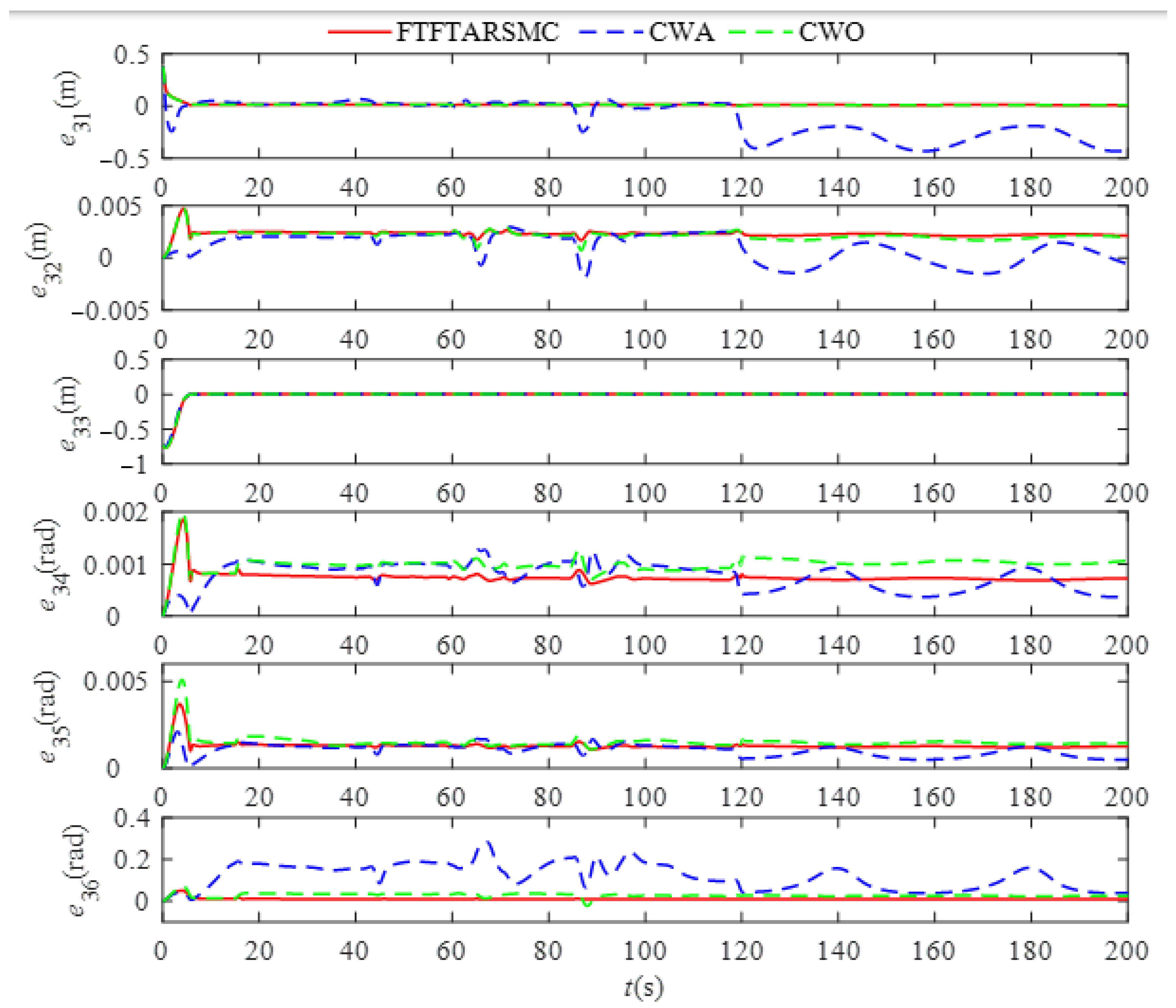
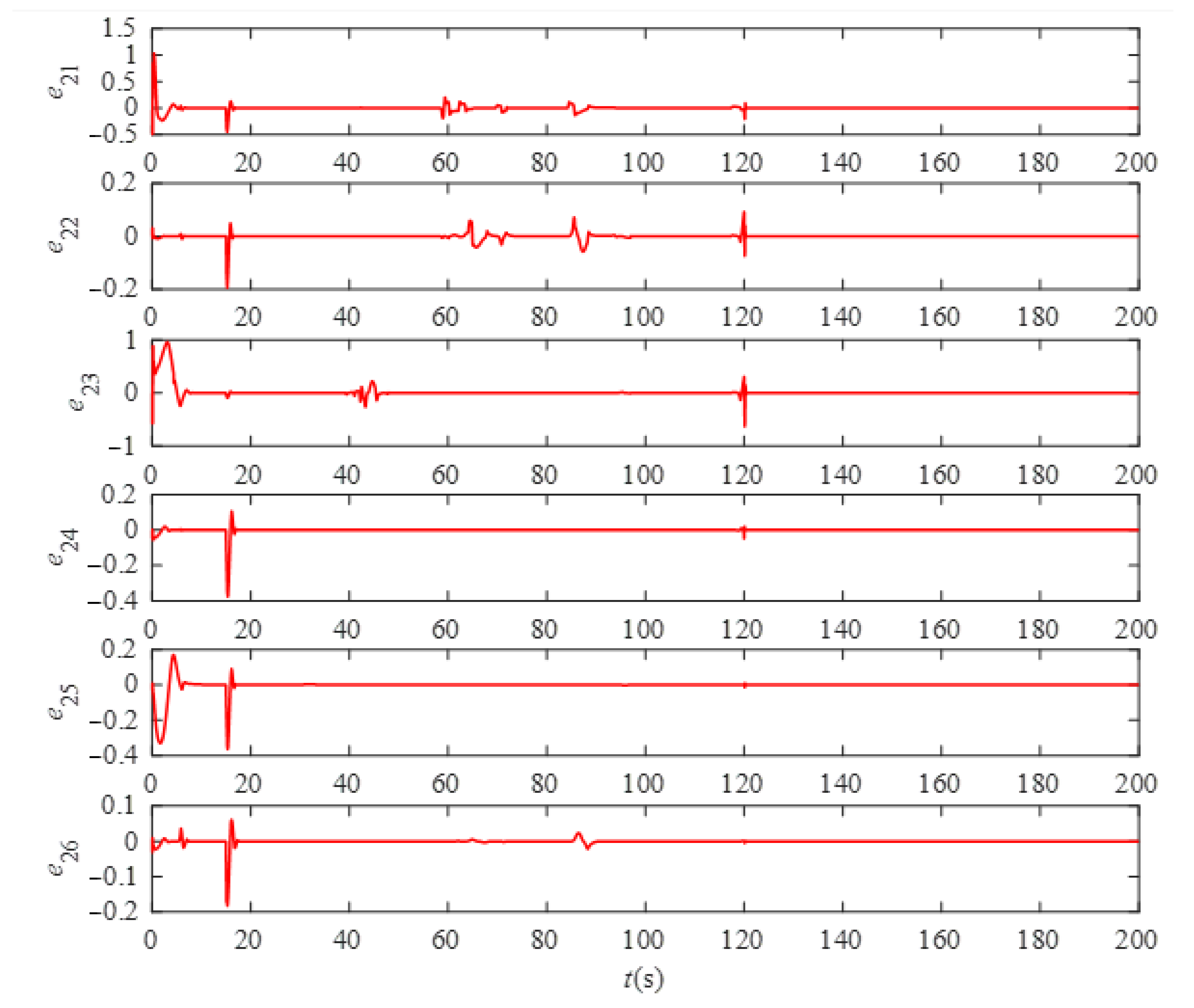
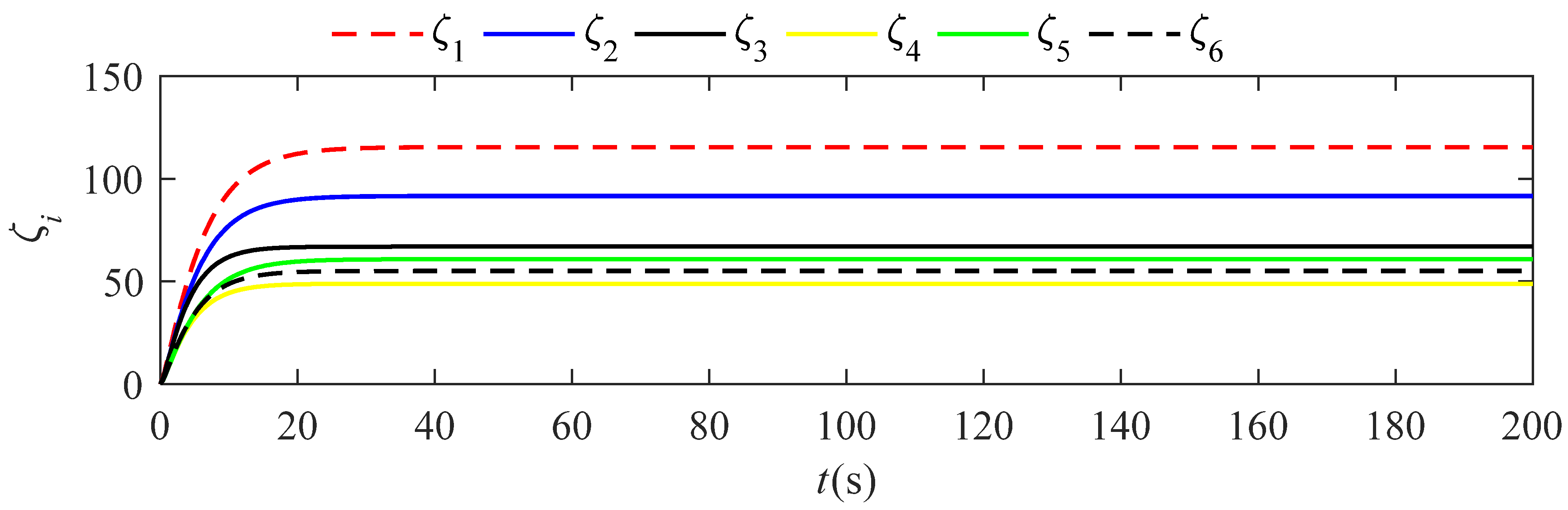
5. Numerical Simulations and Discussions

In this section, the effect of hydrothermal fluids on S-AUVs ${\tau }_d{}_f$ is constructed. The tracking performance of FTFTARSMC algorithms in the TAG mound is verified by numerical simulations.

As shown in Figure 9, the torpedo-type S-AUV has a length of more than 1700 mm, a diameter of 200 mm, and a weight of 70 kg in air. The propulsion system of the S-AUV consists of eight independent thrusters (including two vertical channel thrusters, two vertical conduit thrusters, two lateral channel thrusters, and two main thrusters) to achieve a fully actuated system given in Figure 10. Then, according to the thrust curves, the saturation limits for the main thrusters, channel thrusters, and vertical conduit thruster are roughly taken as ±600 N, ±500 N, and ±150 N, respectively. In the simulation, the thruster outputs from eight thrusters can be obtained in the form of total control forces and moments ${\tau }_v$ at each degree of freedom.

When the S-AUV tracks the designed trajectory near the vents (below 0.6 $Z_{max}$), it suffers from the disturbance ${\tau }_d{}_f$ caused by the hydrothermal plume. Based on the results of the flow field structure for hydrothermal plumes in Refs. [46,47], the direction of cold seawater near the active vents is roughly horizontal to the hydrothermal vent. In addition, the velocity is inversely proportional to the distance from the current position of S-AUVs to the vent in the range with the vent as the center and D ($\mathit{D}\le 30 \mathrm{m}$) as the diameter. However, according to the velocity vector fields of hydrothermal plumes shown in Figure 11, the exact value of the velocity varies depending on the model parameters of plumes.

In addition, there are also some small-scale hydrothermal vents in the TAG active mound. Actually, the effect of small vents can be ignored due to less heat flux and buoyancy flux of the vents. It is worth noting that the S-AUV only suffers from the disturbance ${\tau }_d{}_f$ when sailing above the vent, since the entrainments of hydrothermal plumes have a weak influence on the cold seawater below the vent [45].

According to the above analysis, the disturbance ${\tau }_d{}_f$ is modeled on the earth-fixed frame (E-X₀Y₀Z₀), which can be defined as

$${\tau }_d{}_f{=\mathrm{F}}_{{{}_d}_f}\mathit{J}\left(\mathit{\eta }\right)\left(D-L_1\right)/D if L_1\le D$$

(93)

where $L_1=\sqrt{{\left(x_c-x\right)}^2+{\left(y_c-y\right)}^2+{\left(z_c-z\right)}^2}$ is the distance from S-AUVs to the vent. The resultant force coefficient ${\mathrm{F}}_{{{}_d}_f}$ denotes a small positive constant, since the maximum flow outside plumes is no more than 10 cm/s. For verifying the robustness of FTFTARSMC algorithms, the disturbance ${\tau }_d{}_f$ is appropriately amplified.

The proposed fixed-time fault-tolerant adaptive robust sliding mode controller (FTFTARSMCer) of S-AUVs is applied to the designed trajectory and topography in the TAG hydrothermal mound. In order to evaluate the ability of control algorithms in estimating uncertainties and eliminating saturated constraints, two modified control algorithms based on control laws (72)–(75) will be designed and compared with the proposed FTFTARSMCer, i.e., the proposed controller without the ADS (CWA) and the proposed controller without observers (CWO). The initial variables $\eta \left(0\right)$ and $\upsilon \left(0\right)$ are selected as ${\mathit{\eta }}_1\left(0\right)={\left[126,0,35\right]}^{\mathrm{T}} \mathrm{m}$, ${\eta }_2\left(0\right)={\left[0,0,0\right]}^{\mathrm{T}} \mathrm{rad}$, ${\mathit{\upsilon }}_1\left(0\right)={\left[0,0,0\right]}^{\mathrm{T}} \mathrm{m}/\mathrm{s}$, and ${\mathit{\upsilon }}_2\left(0\right)={\left[0,0,0\right]}^{\mathrm{T}} \mathrm{rad}/\mathrm{s}$. To guarantee the stable operation of sonars, the speed of S-AUVs needs to be controlled within a certain range. The main control parameters are selected in

Table 1. Control parameters for the FTFTARSMCer.

${\beta }_1=0.7$$, {\beta }_2=0.4$$, k=0.09$$, {\epsilon }_0=0.00001$$, C_1=1$$, C_2=1.2$, $C_3=1.2$$, C_4=3$$, \mathit{A}=0.1 \mathrm{diag}\left(0.01,0.1,1.2,0.8,1.9,0.5\right)$,

${\mathit{\beta }}_3=150 \mathrm{diag}\left(0.08,0.01,0.35,0.5,0.24,0.005\right)$,

${\mathit{\beta }}_4=100 \mathrm{diag}\left(0.0001,1.5,0.0001,0.62,0.58,0.001\right)$,

$r_1=0.42$$, r_2=1.4$$, {\epsilon }_1=0.01$$, k_1=0.02 \mathrm{diag}\left(1,0.01,1,8,9,10\right)$,

$k_2=0.022 \mathrm{diag}\left(2.1,2.6,2.7,1.8,2.6,2.8\right)$$, {\lambda }_1=7/5$$, {\lambda }_2=5/7$$, \varpi =0.5$, ${\mu }_1=0.001$$, {\mu }_2=4$$, k_A=0.1$$, k_3=0.00002 \mathrm{diag}\left(1,0.01,1,8,9,10\right)$,

$k_4=0.01 \mathrm{diag}\left(30,0.002,10,1,1,1\right)$$, k_5=0.01 \mathrm{diag}\left(2,2.3,2.01,2.31,1.9,0.1\right)$.

.

In order to reflect the lumped uncertainties (10) in the dynamic model, an additive variance of 40% of the nominal values is considered, i.e., $\mathsf{\Delta }N\left(\mathit{\eta },\mathit{\upsilon }\right)=0.4\left(\widehat{{\rm M}}\dot{\upsilon }+\widehat{C}\left(\mathit{\upsilon }\right)\mathit{\upsilon }+\widehat{\mathit{D}}\left(\mathit{\upsilon }\right)\mathit{\upsilon }+\widehat{g}\left(\eta \right)\right)$. The disturbances ${\tau }_{d\eta }$ are chosen as

$$\begin{array}{l}{\tau }_d{{}_{\eta }}_{,1}=4+3\sin \left(0.3t\right)\mathrm{N},\hspace{1em}{\tau }_d{{}_{\eta }}_{,2}=5\sin \left(0.2t\right)\mathrm{N},\hspace{1em}{\tau }_d{{}_{\eta }}_{,3}=2+4\sin \left(0.1t\right)\mathrm{N},\hspace{1em}\\ {\tau }_d{{}_{\eta }}_{,4}=3+2\cos (0.1t)\hspace{0.17em}\mathrm{N}\mathrm{m}, {\tau }_d{{}_{\eta }}_{,5}=4\cos (0.2t)\mathrm{N}\mathrm{m},\hspace{1em}{\tau }_d{{}_{\eta }}_{,6}=4+\cos (0.3t)\mathrm{N}\mathrm{m}.\end{array}$$

(94)

The conditions of actuator faults are set in

Table 2. Conditions of actuator faults.

eii	0.1 [5;7;7;5;6;7]	t0i	15 [1;1;1;1;1;1]
ai	5 [4;2;1;1;1;3]	${\overline{\tau }}_i$	10 [3;3;3;3;3;3]

.

The trajectory tracking simulation of S-AUVs is created under actuator faults, and the results are presented in Figure 12, Figure 13, Figure 14, Figure 15 and Figure 16. Figure 12 displays the trajectory tracking results under the CWA, CWO, and FTFTARSMCer, respectively. Further, there is little difference between tracking results due to the long-distance trajectory. It can be obviously seen from Figure 13 and Figure 14 that the S-AUV based on the FTFTARSMCer can quickly and stably track the desired trajectory. The CWO can achieve similar control performance on tracking but shows poor performance in terms of control accuracy and stability. Compared with the CWA, the FTFTARSMCer has remarkable performance in the control stability, the extreme value of control input, and the convergence of tracking errors. When the fault occurs at $t_0=\left[15;15;15;15;15;15\right]\mathrm{s}$, the disturbance observer will accurately and quickly estimate the effect of the fault on S-AUVs to improve the robustness of S-AUV systems as shown in Figure 15. From Figure 16, the ADS plays a significant role in the whole control system. From the simulation results, the tracking performance of the fixed-time stable system of S-AUVs is accepted.

In addition, in order to thoroughly compare the performance differences between the CWA, CWO, and FTFTARSMCer, the integral of time multiplied by the absolute error (ITAE), integral time absolute square error (ITASE), and integral of the absolute square error (IASE) are introduced as follows:

$$ITAE={\displaystyle \int \left|e_3\left(t\right)·t\right|}dt, ITASE={{\displaystyle \int t·\left|e_3\left(t\right)\right|}}^{2}dt, IASE={{\displaystyle \int \left|e_3\left(t\right)\right|}}^{2}dt$$

(95)

The error results for the CWA, CWO, and FTFTARSMCer in the actuator fault case are shown in

Table 3. Comparison results.

		ITAE	ITASE	IASE
FTFTARSMCer	e31	206.7718	2.1955	0.0997
	e32	45.3205	0.1031	0.0011
	e33	33.4241	1.9037	1.3802
	e34	14.3956	0.0104	0.0001
	e35	24.8612	0.0309	0.0004
	e36	180.7496	1.6545	0.0243
CWA	e31	325.5508	2.6156	0.1369
	e32	26.7925	0.0471	0.0006
	e33	34.2774	1.9877	1.4256
	e34	14.1360	0.0111	0.0001
	e35	18.7225	0.0196	0.0002
	e36	279.7739	2.6131	0.0644
CWO	e31	193.1567	1.9803	0.0984
	e32	41.1993	0.0862	0.0010
	e33	33.3455	1.8076	1.3446
	e34	20.0825	0.0203	0.0002
	e35	28.9049	0.0421	0.0005
	e36	207.3014	2.1813	0.0379

. From this figure, the FTFTARSMCer provides the minimum value of error results and, thereby, it gives rise to a better performance than CWO and CWA.

6. Conclusions

In the near-bottom explorations of the TAG mound, the S-AUV will suffer from time-varying disturbances, model uncertainties, actuator faults, and input saturations. It is caused by the S-AUV dynamic characteristics, intense hydrothermal activities, and complex terrain. An FTFTARSMC method is proposed to handle these issues. By utilizing the ESO technique, an adaptive FT disturbance observer is constructed to eliminate the effect of lumped uncertainties. To obtain a remarkable fixed-time tracking performance under actuator faults, a continuous fixed-time fast sliding mode surface is designed. It is theoretically verified that fixed-time stabilization for the trajectory tracking system of S-AUVs can be realized with continuous fixed-time adaptive robust controllers. In addition, the simulated terrain is built according to the actual TAG hydrothermal mound, and a smooth trajectory model is constructed by cubic spline interpolation. Finally, comprehensive simulations performed on an actual S-AUV model are given to validate the effectiveness and superiority of the FTFTARSMCer.

In the future, much work needs to be performed, according to Refs [7,23]. We will devote to constructing the semi-physical simulation platform in Unity with C#. The state constraints, model mismatches, and uncertainties of the underactuated AUVs will be considered. Further, we will develop the controller with less computational complexity and computational resources.

References

1. Grenne, T.; Slack, J.F. Mineralogy and geochemistry of silicate, sulfide, and oxide iron formations in Norway: Evidence for fluctuating redox states of early Paleozoic marine basins. Miner. Depos. 2019, 54, 829–848. [Google Scholar] [CrossRef]
2. German, C.R.; Petersen, S.; Hannington, M.D. Hydrothermal exploration of mid-ocean ridges: Where might the largest sulfide deposits be forming? Chem. Geol. 2016, 420, 114–126. [Google Scholar] [CrossRef] [Green Version]
3. Stobbs, I.J. Origins and Implications of Si-Fe Cap Rocks from Extinct Seafloor Massive Sulphide Deposits from the TAG Hydrothermal Field, 26° N, Mid-Atlantic Ridge; University of Southampton: Southampton, UK, 2020. [Google Scholar]
4. Baker, E.T.; German, C.R.; Elderfield, H. Hydrothermal Plumes over Spreading-Center Axes: Global Distributions and Geological Inferences; American Geophysical Union: Malden, MA, USA, 1995; ISBN 978-11-1866-399-8. [Google Scholar]
5. Coogan, L.A.; Seyfried, W.E.; Pester, N.J. Environmental controls on mid-ocean ridge hydrothermal fluxes. Chem. Geol. 2019, 528, 119285. [Google Scholar] [CrossRef]
6. Maki, T.; Horimoto, H.; Ishihara, T.; Kofuji, K. Tracking a sea turtle by an AUV with a multibeam imaging sonar: Toward robotic observation of marine life. Int. J. Control Autom. Syst. 2020, 18, 597–604. [Google Scholar] [CrossRef]
7. Heshmati-Alamdari, S.; Nikou, A.; Dimarogonas, D.V. Robust trajectory tracking control for underactuated autonomous underwater vehicles in uncertain environments. IEEE Trans. Autom. Sci. Eng. 2020, 18, 1288–1301. [Google Scholar] [CrossRef]
8. Zhu, C.; Huang, B.; Zhou, B.; Su, Y.; Zhang, E. Adaptive model-parameter-free fault-tolerant trajectory tracking control for autonomous underwater vehicles. ISA Trans. 2021, 114, 57–71. [Google Scholar] [CrossRef] [PubMed]
9. Zhu, C.; Huang, B.; Su, Y.; Zheng, Y.; Zheng, S. Finite-time rotation-matrix-based tracking control for autonomous underwater vehicle with input saturation and actuator faults. Int. J. Robust Nonlinear Control 2022, 32, 2925–2949. [Google Scholar] [CrossRef]
10. He, S.; Kou, L.; Li, Y.; Xiang, J. Robust Orientation-Sensitive Trajectory Tracking of Underactuated Autonomous Underwater Vehicles. IEEE Trans. Ind. Electron. 2020, 68, 8464–8473. [Google Scholar] [CrossRef]
11. Li, J.; Du, J.; Lewis, F.L. Distributed three-dimension time-varying formation control with prescribed performance for multiple underactuated autonomous underwater vehicles. Int. J. Robust Nonlinear Control 2021, 31, 6272–6287. [Google Scholar] [CrossRef]
12. Wang, H.; Su, B.; Wang, Y.; Gao, J. Adaptive sliding mode fixed-time tracking control based on fixed-time sliding mode disturbance observer with dead-zone input. Complexity 2019, 2019, 8951382. [Google Scholar] [CrossRef] [Green Version]
13. Qin, H.; Yang, H.; Sun, Y.; Zhang, Y. Adaptive Interval Type-2 Fuzzy Fixed-time Control for Underwater Walking Robot with Error Constraints and Actuator Faults Using Prescribed Performance Terminal Sliding-mode Surfaces. Int. J. Fuzzy Syst. 2020, 23, 1137–1149. [Google Scholar] [CrossRef]
14. Chen, Z.; Yang, X.; Liu, X. RBFNN-based nonsingular fast terminal sliding mode control for robotic manipulators including actuator dynamics. Neurocomputing 2019, 362, 72–82. [Google Scholar] [CrossRef]
15. Ning, W.; Meng, J.E. Direct Adaptive Fuzzy Tracking Control of Marine Vehicles With Fully Unknown Parametric Dynamics and Uncertainties. IEEE Trans. Control Syst. Technol. 2016, 24, 1845–1852. [Google Scholar] [CrossRef]
16. Wang, N.; Karimi, H.R.; Li, H.; Su, S. Accurate Trajectory Tracking of Disturbed Surface Vehicles: A Finite-Time Control Approach. IEEE/ASME Trans. Mechatron. 2019, 24, 1064–1074. [Google Scholar] [CrossRef]
17. Peng, Z.; Wang, J. Output-Feedback Path-Following Control of Autonomous Underwater Vehicles Based on an Extended State Observer and Projection Neural Networks. IEEE Trans. Syst. Man Cybern. Syst. 2017, 48, 535–544. [Google Scholar] [CrossRef]
18. Yang, X.; Yan, J.; Hua, C.; Guan, X. Trajectory Tracking Control of Autonomous Underwater Vehicle With Unknown Parameters and External Disturbances. IEEE Trans. Syst. Man Cybern. Syst. 2019, 51, 1054–1063. [Google Scholar] [CrossRef]
19. Huang, B.; Zhou, B.; Zhang, S.; Zhu, C. Adaptive prescribed performance tracking control for underactuated autonomous underwater vehicles with input quantization. Ocean Eng. 2021, 221, 108549. [Google Scholar] [CrossRef]
20. Zhu, C.; Zeng, J.; Huang, B.; Su, Y.; Su, Z. Saturated approximation-free prescribed performance trajectory tracking control for autonomous marine surface vehicle. Ocean Eng. 2021, 237, 109602. [Google Scholar] [CrossRef]
21. Yoerger, D.R.; Cooke, J.G.; Slotine, J.J. The influence of thruster dynamics on underwater vehicle behavior and their incorporation into control system design. IEEE J. Ocean. Eng. 1990, 15, 167–178. [Google Scholar] [CrossRef] [Green Version]
22. Di Vito, D.; Cataldi, E.; Di Lillo, P.; Antonelli, G. Vehicle adaptive control for underwater intervention including thrusters dynamics. In Proceedings of the 2018 IEEE Conference on Control Technology and Applications (CCTA 2018), Copenhagen, Denmark, 21–24 August 2018; pp. 646–651. [Google Scholar]
23. Bechlioulis, C.P.; Karras, G.C.; Heshmati-Alamdari, S.; Kyriakopoulos, K.J. Trajectory tracking with prescribed performance for underactuated underwater vehicles under model uncertainties and external disturbances. IEEE Trans. Control Syst. Technol. 2016, 25, 429–440. [Google Scholar] [CrossRef]
24. Cui, R.; Zhang, X.; Cui, D. Adaptive sliding-mode attitude control for autonomous underwater vehicles with input nonlinearities. Ocean Eng. 2016, 123, 45–54. [Google Scholar] [CrossRef]
25. Li, J.; Du, J.; Chang, W.J. Robust time-varying formation control for underactuated autonomous underwater vehicles with disturbances under input saturation. Ocean Eng. 2019, 179, 180–188. [Google Scholar] [CrossRef]
26. Liu, X.; Zhang, M.; Yao, F. Adaptive fault tolerant control and thruster fault reconstruction for autonomous underwater vehicle. Ocean Eng. 2018, 155, 10–23. [Google Scholar] [CrossRef]
27. Liu, X.; Zhang, M.; Wang, Y.; Rogers, E. Design and Experimental Validation of an Adaptive Sliding Mode Observer-Based Fault-Tolerant Control for Underwater Vehicles. IEEE Trans. Control. Syst. Technol. 2018, 27, 2655–2662. [Google Scholar] [CrossRef]
28. Guerrero, J.A.; Torres, J.; Creuze, V.; Chemori, A. Adaptive disturbance observer for trajectory tracking control of underwater vehicles. Ocean Eng. 2020, 200, 107080. [Google Scholar] [CrossRef] [Green Version]
29. Fossen, T.I. Handbook of Marine Craft Hydrodynamics and Motion Control; John Wiley & Sons: New York, NY, USA, 2011; ISBN 978-11-1999-149-6. [Google Scholar]
30. Ning, W.A.; Xp, B.; Sfs, C. Finite-time fault-tolerant trajectory tracking control of an autonomous surface vehicle. J. Frankl. Inst. 2020, 357, 11114–11135. [Google Scholar] [CrossRef]
31. Galley, C.; Lelievre, P.; Haroon, A.; Graber, S.; Jamieson, J.; Szitkar, F.; Yeo, I.; Farquharson, C.; Petersen, S.; Evans, R. Magnetic and gravity surface geometry inverse modeling of the TAG active mound. J. Geophys. Res. Solid Earth 2021, 126, e2021JB022228. [Google Scholar] [CrossRef]
32. Lupton, J.E. Hydrothermal plumes: Near and far field. Seafloor Hydrothermal Syst. Phys. Chem. Biol. Geol. Interact. 1995, 91, 317–346. [Google Scholar] [CrossRef]
33. Zhiguo, H.E.; Han, X.Q.; Qiu, Z.Y.; WANG, Y.; QIU, Z. Numerical modeling of hydrodynamic processes of deep-sea hydrothermal plumes: A case study on Daxi hydrothermal field, Carlsberg Ridge. Sci. Sin. Technol. 2020, 50, 194–208. [Google Scholar] [CrossRef] [Green Version]
34. PMEL Earth-Ocean Interactions Program, Axial Seamount. 2021. Available online: https://www.pmel.noaa.gov/eoi/chemistry/fluid.html (accessed on 5 March 2021).
35. Zheng, Z.; Feroskhan, M.; Sun, L. Adaptive fixed-time trajectory tracking control of a stratospheric airship. ISA Trans. 2018, 76, 134–144. [Google Scholar] [CrossRef]
36. Deng, H.; Krstić, M. Stochastic nonlinear stabilization—I: A backstepping design. Syst. Control Lett. 1997, 32, 143–150. [Google Scholar] [CrossRef]
37. Huang, Y.; Jia, Y. Robust adaptive fixed-time tracking control of 6-DOF spacecraft fly-around mission for noncooperative target. Int. J. Robust Nonlinear Control 2018, 28, 2598–2618. [Google Scholar] [CrossRef]
38. Liang, K.; Lin, X.; Chen, Y.; Li, J.; Ding, F. Adaptive sliding mode output feedback control for dynamic positioning ships with input saturation. Ocean Eng. 2020, 206, 107245. [Google Scholar] [CrossRef]
39. Tang, P.; Lin, D.; Zheng, D.; Fan, S.; Ye, J. Observer based finite-time fault tolerant quadrotor attitude control with actuator faults. Aerosp. Sci. Technol. 2020, 104, 105968. [Google Scholar] [CrossRef]
40. Zhu, G.; Du, J. Robust adaptive neural practical fixed-time tracking control for uncertain Euler-Lagrange systems under input saturations. Neurocomputing 2020, 412, 502–513. [Google Scholar] [CrossRef]
41. Plestan, F.; Shtessel, Y.; Bregeault, V.; Poznyak, A. New methodologies for adaptive sliding mode control. Int. J. Control 2010, 83, 1907–1919. [Google Scholar] [CrossRef] [Green Version]
42. Ullah, S.; Khan, Q.; Mehmood, A.; Kirmani, S.A.M.; Mechali, O. Neuro-adaptive fast integral terminal sliding mode control design with variable gain robust exact differentiator for under-actuated quadcopter UAV. ISA Trans. 2021, 120, 293–304. [Google Scholar] [CrossRef]
43. Cruz-Ortiz, D.; Chairez, I.; Poznyak, A. Non-singular terminal sliding-mode control for a manipulator robot using a barrier Lyapunov function. ISA Trans. 2021, 121, 268–283. [Google Scholar] [CrossRef]
44. Humphris, S.E.; Tivey, M.K.; Tivey, M.A. The Trans-Atlantic Geotraverse hydrothermal field: A hydrothermal system on an active detachment fault. Deep. Sea Res. Part II Top. Stud. Oceanogr. 2015, 121, 8–16. [Google Scholar] [CrossRef] [Green Version]
45. Graber, S.; Petersen, S.; Yeo, I.; Szitkar, F.; Klischies, M.; Jamieson, J.; Stobbs, I. Structural control, evolution, and accumulation rates of massive sulfides in the TAG hydrothermal field. Geochem. Geophys. Geosystems 2020, 21, e2020GC009185. [Google Scholar] [CrossRef]
46. Jiang, H.; Breier, J.A. Physical controls on mixing and transport within rising submarine hydrothermal plumes: A numerical simulation study. Deep. Sea Res. Part I Oceanogr. Res. Pap. 2014, 92, 41–55. [Google Scholar] [CrossRef]
47. Matulka, A.; López, P.; Redondo, J.M.; Tarquis, A. On the entrainment coefficient in a forced plume: Quantitative effects of source parameters. Nonlinear Processes Geophys. 2014, 21, 269–278. [Google Scholar] [CrossRef] [Green Version]
Figure 1. Body-fixed motion frame (G-XYZ) and earth-fixed frame (E-X0Y0Z0) for an AUV.
Jmse 10 00721 g001
Figure 2. The active TAG hydrothermal field [31].
Jmse 10 00721 g002
Figure 3. The hydrothermal plume [34].
Jmse 10 00721 g003
Figure 4. The built TAG hydrothermal mound.
Jmse 10 00721 g004
Figure 5. The path in the TAG mound.
Jmse 10 00721 g005
Figure 6. Comparison of trajectory models and paths in horizontal and vertical planes.
Jmse 10 00721 g006
Figure 7. (a) The single error result between the trajectory model and the path, (b) The difference between the trajectory model and the path in the vertical descent region.
Jmse 10 00721 g007
Figure 8. The whole desired trajectory.
Jmse 10 00721 g008
Figure 9. The drawing of torpedo-type S-AUVs.
Jmse 10 00721 g009
Figure 10. (a) The propulsion system of the S-AUV in the side view, (b) The propulsion system of the S-AUV in the vertical view.
Jmse 10 00721 g010
Figure 11. The flow field characteristics of hydrothermal plume.
Jmse 10 00721 g011
Figure 12. Trajectory tracking of the S-AUV.
Jmse 10 00721 g012
Figure 13. Control input.
Jmse 10 00721 g013
Figure 14. Position and attitude tracking errors.
Jmse 10 00721 g014
Figure 15. Observation errors.
Jmse 10 00721 g015
Figure 16. The state of the auxiliary system.
Jmse 10 00721 g016