Abstract
The unmanned surface vehicle (USV) is significantly affected by the ocean environment and weather conditions when navigating. The energy consumption is large, which is not conducive to completing water tasks. This study investigates the global energy-efficient path planning problem for the USV, wherein the goal is to obtain an optimal path under the interference of the ocean environment and control the USV to avoid static obstacles and arrive at its destination. Firstly, this paper extracts the coastline coordinates and water depth data from the S-57 electronic chart, applying the Voronoi diagram to describe spatial object information preliminarily. Secondly, the dynamic, safe water depth model is obtained using the improved Voronoi diagram algorithm after superimposing the interpolated tide with the water depth data. In order to construct the total energy consumption model, the mathematical model of wind and current is introduced into the linear dynamics model of a USV. Additionally, the timing breakpoints are planned. According to the energy consumption model, this paper improves the A* algorithm to replan the path to consider the distance costs and variation of ocean data in each timing breakpoint. Finally, this paper proposes a new path optimization algorithm to reduce the waypoints and smooth the path. Simulations verified the effectiveness of the method. The energy consumption in a favorable situation is less than in a counter situation. The higher the USV velocity, the higher the energy consumption. The proposed dynamic energy-efficient path considers the distance, ensures a shorter range, and improves the endurance of the USV, which is in line with the actual navigation requirement.
1. Introduction
1.1. Research Background
In the 21st century, humanity has entered a period of large-scale exploitation and utilization of the ocean. The ocean plays a crucial role in economic development patterns. It is necessary to enhance the ability to explore marine resources and strengthen the protection of coastal zones and the marine ecological environment. However, there are many problems in the traditional offshore operation mode. For example, conventional hydrological exploration adopts the artificial method, which requires professional sampling or exploration personnel to take samples at sea for experimental analysis. As a result, the cost is high, the efficiency is too slow, and the natural conditions are easy to limit. Therefore, it is not easy to achieve large-scale and continuous detection. Traditional operations to safeguard national maritime sovereignty, such as port security, guard patrol, and maritime search and rescue, mainly rely on the support of large sums of money platforms, which are costly and risky. With the intellectual development of marine equipment, unmanned monitoring platforms should arrive. The unmanned surface vehicle (USV) [1,2,3] is one of the small surface boats widely used in maritime mapping, hydrological monitoring, maritime surveillance reconnaissance, anti-mine warfare, and other military and civilian fields. It provides convenience for real-time control of marine dynamics and monitoring the marine environment. The USV is typically modular in design, enabling it to perform different tasks. Its high speed and high maneuverability allow it to quickly navigate specific waters, such as shallow water and narrow lanes, which cannot be reached by conventional vessels. It dramatically expands the scope of operation and has a low cost [4]. In addition, the USV is favored in developing and applying intelligent marine inspection equipment because they can be deployed in large numbers and perform more dangerous missions without human exposure.
When performing specific navigation missions, the USV must navigate autonomously according to preset paths and perform tasks, such as terrain survey, mine clearance, water quality sampling, and visual monitoring. This kind of task needs to rely on the autonomous navigation control system of the USV to achieve this. At the same time, the system’s stability also determines the difficulty of completing the task. The autonomous navigation control system mainly has three core parts: guidance, navigation, and control [5]. Among them, the guidance system is the critical technology used by the USV, which requires that under certain constraints, it has the safest, shortest range, and the most energy-efficiency, and that it can automatically plan a stable, continuous, and accessible path from start to finish based on assigned tasks, environmental conditions, and navigation information. It includes global path planning with general environment information and local path planning with unknown environment information and path adjustment. However, the current path planning technology mainly studies the safest and shortest distance, ignoring the energy consumption of the USV. Planning the shortest path does not necessarily mean the lowest energy consumption. Navigating against the wind and current will lose much energy and the UAV may even fail to reach its destination. A long endurance time and low energy consumption are critical USV requirements in surface operation tasks, especially in extensive sea area exploration. Therefore, the ability of the USV to operate at sea for long periods is needed. Energy consumption is usually reduced by developing more efficient electricity supplies or exploiting the environment. However, path planning considers the marine environment less, such as the interference of the wind and current on the hull. Because the USV is small in size, anti-jamming and low range of problems in its mission may not be able to effectively track the given path, which deviates from the route, causing unnecessary energy waste and even possible risk of collision. Therefore, this paper proposes an hourly dynamic energy-efficient path planning algorithm that considers the distance.
1.2. Related Studies
As one of the USV’s critical technologies, path planning has become a hot topic for scholars at home and abroad. Many different methods have been proposed in the research field for improving endurance by taking energy-saving as a planning index. The three steps of path planning: environment modeling, path search, and path optimization are discussed.
The environmental modeling steps include selecting modeling methods with high modeling accuracy and high speed. Standard modeling methods include the raster and geometric modeling methods [6]. There are many pieces of research based on the raster method, and the modeling effect of the raster method is very dependent on the size of the grid. If the grid is too large, the accuracy will decrease. Otherwise, too many small grids will significantly reduce the running speed. Therefore, it is suitable for spatial modeling in robots or small sea areas [7]. Lee T et al. [8] proposed a navigation system based on waypoints to establish 3D path planning by considering the ocean environment’s influence, such as the tide and water depth, the ship’s steering performance, and the ship’s attitude at the port of origin and destination. By improving the A* algorithm, the influences of the current and shallow water effect is introduced into the edge cost function to carry out path planning, and ensures that the USV can fulfill the requirements of offshore operations with minimum energy consumption in a large sea area.
However, there are still some problems, such as the grid method, which results in a considerable calculation time. In addition, the time variation of the current cannot simply be superimposed on the vessel speed, and the influence of the wind and dynamic model of the ship is not considered, therefore, the generated path has a low real reference value. Methods based on geometric modeling mainly include the Voronoi diagram and Visibility diagram [4,9]. The Voronoi diagram has the advantage of fast computing speeds compared with the Visibility diagram. The operation time of vertices is , while that of the Visibility diagram is . Therefore, the Voronoi diagram is more suitable for large spatial data sets. In addition, the Voronoi diagram has higher security, while the Visibility diagram has a particular risk because it is linked to all the vertices. Niu H et al. [10] described the properties of Voronoi diagrams and Visibility diagrams by analyzing the computational efficiency, extending the coastline to a safe distance, and building a preliminary environmental model using the Voronoi diagram. The USV energy consumption model was constructed by analyzing the influence of ocean currents. They were using the Dijkstra algorithm to plan energy-efficient paths. Finally, they generated multiple candidate paths by combining the Visibility diagram and the Dijkstra algorithm to search for the optimal energy-efficient path. The simulation analysis of the Voronoi–Visibility energy-efficient path (VVEE) and Voronoi–Visibility shortest path took place in the Singapore Strait and Croatia sea. The energy-efficient path is more advantageous than the conventional path under prominent ocean current variation, downstream, and low-speed navigation. The method retains the computational efficiency of the Voronoi diagram and combines the Visibility diagram’s optimization effect. However, the article still does not consider the impact of wind variation on the movement of the USV. In addition, tidal changes are also a critical factor when navigating in straits with many islands and reefs, which should be comprehensively considered to generate an energy-efficient and safe path.
There are many representative algorithms in the path search algorithm and an optimization module. Path planning algorithms, based on graphics, mainly include Dijkstra [11] and the A* algorithm [12]. Garau B et al. [13] proposed an efficient path planning algorithm based on A*, considering current ocean data. However, the A* algorithm needs enormous computing power and is difficult to deal with high-dimensional problems. Bionics path planning algorithms include the ant colony algorithm [14], genetic algorithm [15], and particle swarm optimization algorithm [16]. Liu, Xinyu, et al. [17] proposed an automatic obstacle avoidance algorithm based on an ant colony algorithm and clustering algorithm to solve the problem of how to use multi-information integration to realize large-scale dynamic path planning at sea. Firstly, they matched different environmental complexities of the clustering algorithm, automatically selected the appropriate search scope and improved the path planning performance. Then, the path smoothing mechanism was introduced to meet the USV feature constraints. At the same time, using the ant colony algorithm for local path planning and applying multi-source information positioning realized the designated waters adaptive recognition, obstacle warning, and dynamic obstacle avoidance path planning. However, the algorithm does not consider the influence of the marine environment and weather conditions, nor does it consider the kinematic constraints of the USV, which does not meet the requirements of the natural navigation environment. Ding F.et al. [18] proposed an efficient and energy-saving path-planning and path-tracking control method based on a particle swarm optimization algorithm for navigation safety and energy consumption in the complex ocean environment. They established the USV motion mathematical model and marine environment mathematical model. Modeling, using electronic chart information and environmental information with appropriate objective function and constraint conditions, using the particle swarm optimization algorithm, obtained the energy-saving path, real-time route replanning, and adjustment as weather conditions changed. Finally, they used a particle swarm optimization algorithm to control the generated energy-saving path with potential induced degradation (PID). The optimal control parameters were obtained. The approximate method sets the ocean current as a constant and does not effectively consider the time-varying characteristics of the ocean current. Sample-based path planning includes a rapidly-exploring random tree algorithm (RRT) [19]. Kamarry S et al. [20] generated a cost-effective path through the path planning algorithm of the RRT algorithm to meet the task requirements of linear time logic. The cost function includes the hazard level, energy consumption, and wireless connection. Reducing node redundancy and the number of discarded samples minimizes the tree growth’s processing time, and thus, the computational cost shortens the path length and saves energy. However, the RRT algorithm has great randomness, making the generated path unstable.
Finally, energy-efficient path planning methods in other fields were summarized: Wang Y et al. [21] focused on the representation and avoidance strategies of obstacles in the task environment. They defined the obstacle area as an inner circle and an outer circle, and the area was divided according to the tangent line from the two loops to the starting point to limit the unmanned aerial vehicle’s (UAV) flight area so that the UAV could avoid the obstacle and achieve minimum propulsion energy consumption. A path planning method based on a multi-agent is proposed to generate feasible paths from candidate sets. Li, Deshi, et al. [22] used a genetic algorithm to traverse the energy consumption graph in 3D in an outdoor environment to avoid local optimization. They combined the model with the energy consumption estimation equation as the input of the energy consumption graph to obtain the optimal energy path. Deepak N. [23] proposed a method based on the stochastic level set partial differential equations (PDEs) to calculate relative velocity and relative heading, rigorously predicting the optimal energy path in deterministic dynamic flows. It can be used to calculate the optimal energy path of the AUV time-optimal path in the dynamic flow field. Yu H et al. [24] proposed a fast marching method for AUV path planning in a large-scale three-dimensional environment. For AUV navigation path safety, fuel consumption, navigation, and other problems involving optimization modeling, it considers the collision risk between obstacles and mines, detection probability, navigation depth, route length, and the maneuvering constraints of AUV, including a safe depth and turning radius. Yilmaz et al. [25] introduced a mixed-integer linear programming (MILP) path planning algorithm to navigate multiple AUVs. However, the calculation time of this method will increase exponentially with the size of the problem, so the natural navigation environment will limit this method. Dynamic programming and MILP may not be computationally feasible when USV path planning is performed in a spatio-temporal ocean current environments.
Different types of algorithms were optimized to reduce energy consumption in the path planning research with energy consumption as the index above. However, maritime route planning faces more complex interference factors than UAVs and unmanned ground vehicles. The above algorithms do not comprehensively consider the influencing factors of USV navigation, such as the interaction between the ocean environment and the vessel and the processing ability of large data sets during navigation in a large sea area. Therefore, this paper proposed a dynamic energy-efficient path planning algorithm that considers the distance under the time-varying wind and current. A Voronoi diagram with high computational speed and maximum security is selected, inspired by Niu H et al. [4,10]. However, since the Voronoi diagram generates fewer turning points and navigable paths than other modeling methods [26], part of the extracted safe water depth points are included in the structure to generate more navigable paths. The environmental model is updated hourly to consider the temporal variation of tide, wind, and currents. In addition, the current and wind model was added to the dynamic model of the USV to establish the energy consumption model. The energy consumption is simulated in the same way as USV thrust work. Each waypoint’s energy value is effectively stored in the adjacency matrix, making the subsequent path planning more convenient. The A* algorithm is improved to search for a path with minor energy consumption and a short distance. Finally, the path optimization algorithm reduces the waypoints. The dynamic energy-efficient path algorithm considers the distance, ensures low energy consumption, does not sacrifice a high distance cost, and improves the endurance of the USV.
The structure of this paper is as follows: Section 2 describes the problems to be solved in energy-efficient path planning. Section 3 introduces the mathematical methods and model construction used in this paper in detail. In Section 4, the proposed method is experimentally verified. Section 5 is the experimental conclusion and future work.
2. Question
The following three problems must be considered when the USV carries out long-distance operations at sea:
- Long-distance navigation means an extensive spatial data set. It is essential to select an appropriate modeling method to reduce the computing time of large data sets, as introduced in Section 2.2.
- The USV can not be simplified as a mass point, ignoring its motion characteristics, introduced in Section 2.3.
- The influence of marine environmental factors on the USV and environmental factors changing with time must be considered when navigating a long distance.
2.1. Assumptions
To comprehensively consider the motion of the USV and the marine environment effect, the paper proposed the following hypotheses:
- This paper studies global energy-efficient path planning and does not consider dynamic obstacles.
- This paper first considers the impact of wind and current because of the complex effects of waves on the USV, assuming that the wind and current are constant within each hour.
- The USV motion is specified in two-dimensional space. Hence the motion of the USV in roll, pitch, and heave direction was neglected.
- The USV had neutral buoyancy, and the origin of the body-fixed coordinate was located at the center of the mass.
2.2. Large Data Set
It is essential to select a suitable modeling method because of the substantial spatial data set required for USVs sailing. Standard space modeling methods include the grid, Voronoi diagram, and Visibility diagram [4]. The grid method requires the artificial setting of grid accuracy, which often determines the final path planning effect. For example, high accuracy of grid setting requires a lot of operation time. The low precision of the setting will cause problems, such as a fuzzy environment and a rough route. Compared with the Visibility diagram, the Voronoi diagram has the advantages of fast computing speed and higher path security. It is more suitable for large spatial data sets [10]. The Voronoi diagram is selected to describe spatial object information in this paper. More importantly, the improved Voronoi graph algorithm is more suitable for time-varying spatial modeling.
2.3. USV Model
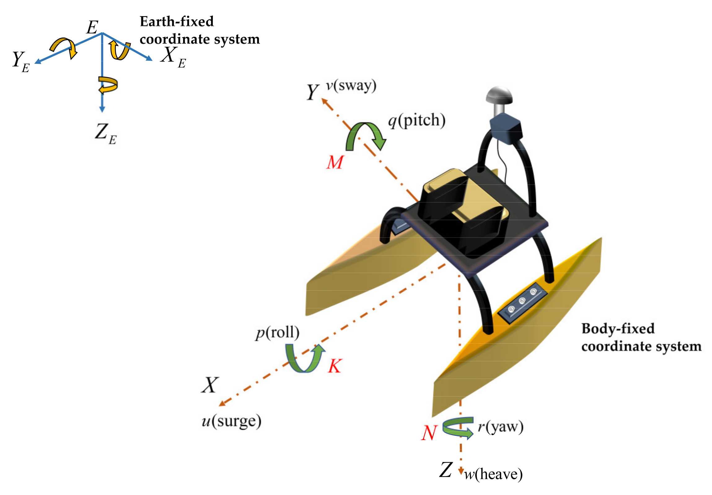
The USV will produce motion in six degrees of freedom when navigating: roll (X-rotation) pitch (Y-rotation), yaw (Z-rotation), sway (sideways motion), surge (longitudinal motion), and heave (vertical motion) [27]. As shown in Figure 1, there are two coordinate systems, the earth-fixed coordinate system, and the body-fixed coordinate system. There is a transformation relationship between the two coordinate systems. For the high-speed USV, the force and motion characteristics will be more prominent in the direction of six degrees of freedom. Therefore, it is necessary to analyze the motion characteristics of the USV in different degrees of freedom rather than regard it as a particle. This paper simplifies the six degrees of freedom into three degrees in a two-dimensional plane: yaw, sway, and surge. The three degrees of freedom (3DOF) dynamics model of the USV is established to analyze its forces at sea.
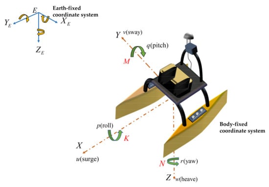
Figure 1.
Motion variables for USV.
2.4. Environment Effect
The first step in path planning is to build an accurate environment model. The S-57 chart extracts obstacle points to create an unnavigable area. The endurance of the USV is limited by the ocean environment (wind and current) in long-distance sailing. It is dangerous to navigate against the wind and current. The USV will bear greater energy consumption and even fail to reach the target point. Considering the influence of wind and current, the USV will automatically sail in the direction of weak wind and current, but it may sacrifice the distance. Therefore, considering energy efficiency and distance cost, it can ensure safe navigation, save energy consumption, and meet the mission requirements of long-distance navigation at sea.
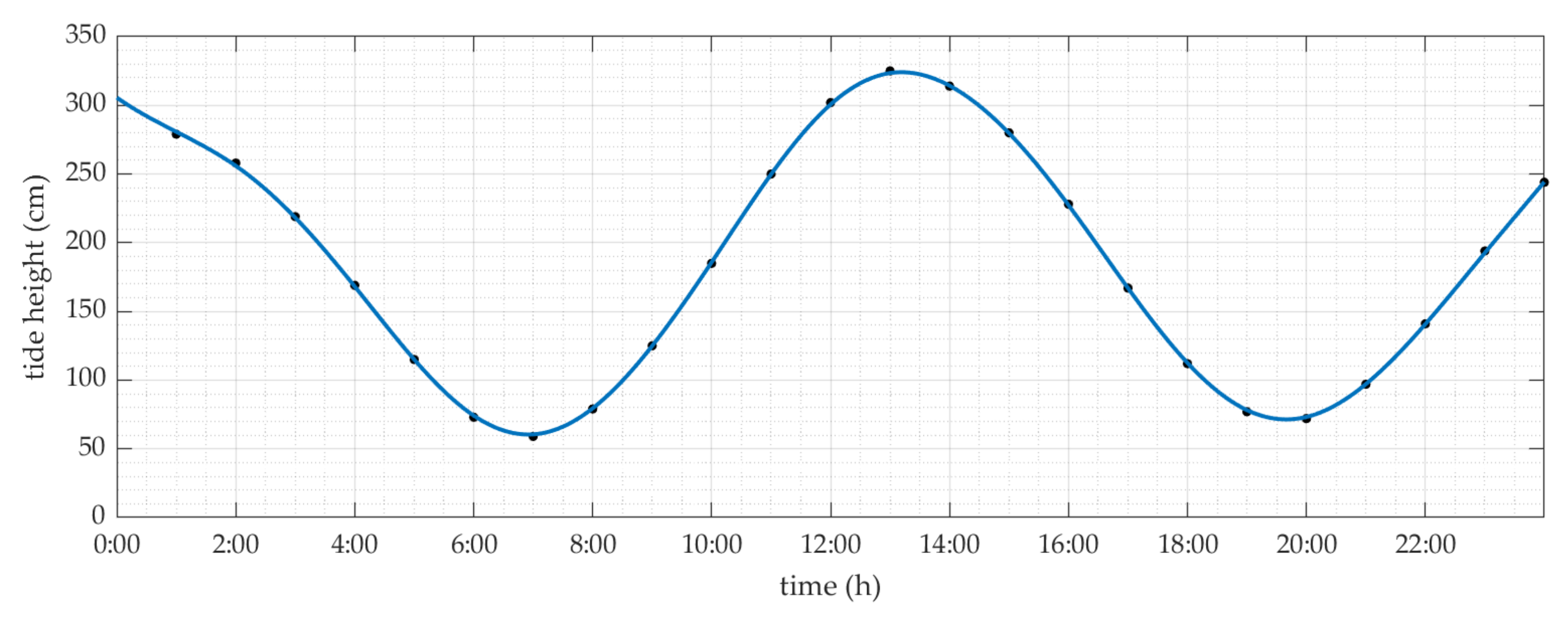
In this paper, the tide table of Dalian port on 20 July 2019, was obtained from the tide prediction table, as shown in Figure 2. In addition, the wind and current data were used in the Bohai Sea in July 2019. The range of the wind data is (119.0455° E–122.9318° E, 36.0818° N–39.9659° N), which is obtained from the National centers for environment prediction (NCEP) climate forecast system, version 2 (CFSv2) data. The current data was obtained from the global hybrid coordinate ocean model (HUCOM) with the range (118.96–122.96° E, 36–40° N). The current and wind data variables are shown in Table 1 and Table 2.
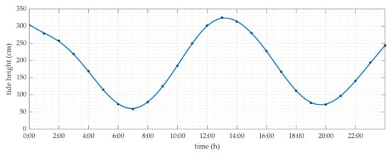
Figure 2.
The tide table.

Table 1.
The current data.
Table 2.
The wind data.
3. Methodology
This chapter is mainly composed of the following parts: Section 3.1 describes the central architecture of this article. Section 3.2 includes the method of data set extraction and the model construction process of the wind and current used in this paper. Section 3.3 introduces the dynamics model of the USV to prepare for the subsequent energy consumption model. Section 3.4 deduces the USV energy consumption in 3DOF, which is the major innovation part. The Voronoi diagram’s generation process and the improved Voronoi diagram algorithm are used to construct dynamic environment modeling, introduced in Section 3.5. Section 3.6 introduces the division of timing breakpoints, the improved A* algorithm and proposes a new optimization algorithm to reduce the waypoints.
3.1. Algorithm Architecture
As shown in Figure 3, based on the coastline contour data and water depth data of electronic charts, this paper describes spatial object information through the Voronoi diagram and preliminarily builds a static navigation environment model. After interpolating tidal level information and the static water depth value, the dynamic safe water depth model is obtained using the improved Voronoi diagram algorithm. The mathematical model of wind and current is introduced into the linear dynamics model of the USV to construct the total energy consumption model. The timing breakpoint is planned according to the general mission voyage to consider wind and current time variation. This paper applies an improved A* algorithm to replan the path according to the timing breakpoint to consider the distance costs and obtain the dynamic energy-efficient path that considers the distance. In the final path optimization stage, this paper carried out a new path optimization to reduce the number of waypoints and smooth the path.
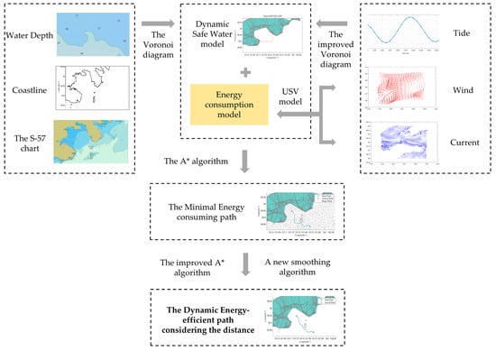
Figure 3.
The proposed dynamic energy-efficient path planning architecture considers the distance algorithm.
3.2. Environment Data Set
This section introduces the basic theory used in deriving the energy consumption model. The marine environment is mainly composed of geographic information and marine hydrometeorological information. The geographic information is mainly coastline contour points introduced in Section 3.2.1. Under the condition of safe obstacle avoidance, the hydrometeorological information of the USV has a significant influence on the navigation movement, including wind, current, sea fog, tide, wind wave, surge wave, and water depth information. Because of the complexity of wave variation with time, this paper mainly studies the relatively uniform and steady media of tidal, wind, and current, introduced in Section 3.2.2, Section 3.2.3 and Section 3.2.4, respectively. We established the mathematical model of wind and current and analyzed the forces and torques acting on 3DOF.
3.2.1. Coastline Data
This paper studies global energy-efficient path planning. Accurate static obstacle modeling is essential. Compared with the Global Self-consistent High-Resolution Shorelines (GSHHS) data set, the coastline data set extracted from the S-57 electronic chart is more accurate and does not require obstacle swelling processing. The process of data extraction is shown in Figure 4.
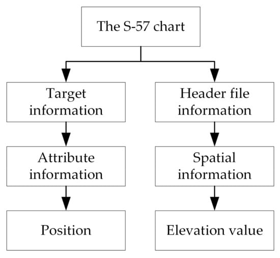
Figure 4.
The S-57 Electronic Chart data reading flow.
The specific process is:
- Extracting header file information and object target information from the S-57 electronic chart file.
- Continue to extract and analyze spatial information and attribute information.
- The spatial and attribute information is converted into the longitude and latitude of obstacles and elevation values.
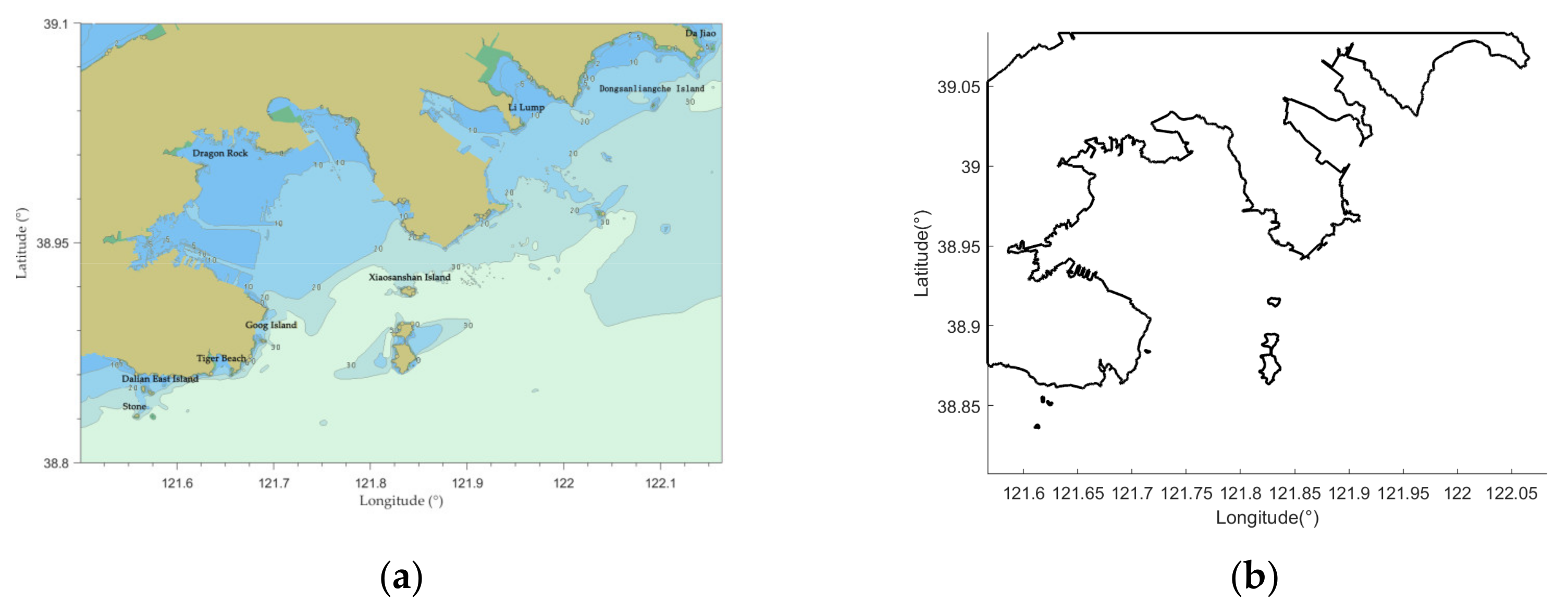
In this paper, the No. C1513431 chart is used to extract the coastline coordinates. The coordinates of the lower-left corner of the sea area are (121.5667, 38.8067), and the upper right corner is (122.0833, 39.0833). The contours of the coastline before and after extraction are shown in Figure 5.
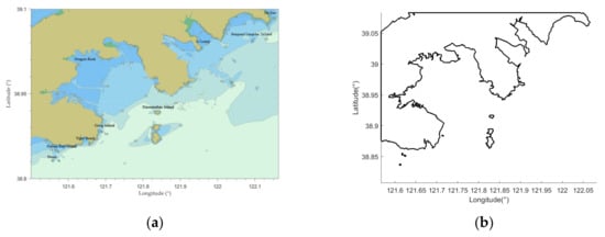
Figure 5.
(a) The S-57 Electricity Chart. (b) The coastline data was extracted from the S-57 electricity chart.
3.2.2. Tide Data
Tidal variation will constantly affect the bathymetric environment and the overall path planning result. This paper builds the dynamic navigation water depth model to obtain the natural navigation environment. At present, the public tide data contains the time and height. Based on the first law of geography, namely spatial correlation, the kriging interpolation method [28] is used to interpolate the tide data. The tide data corresponding to each water depth point is obtained:
where is the predicted tide value at point X and is the weight coefficient. The weighted sum of data of all known points in space is used to estimate the value of unknown points, which satisfies a set of optimal coefficients with the slightest difference between the estimated value and the actual value at the point .
Constructing cost function:
Let the semi-variance function and the constraint obtain the function:
Find the smallest group, and take the partial derivative of the constructor to list the matrix.
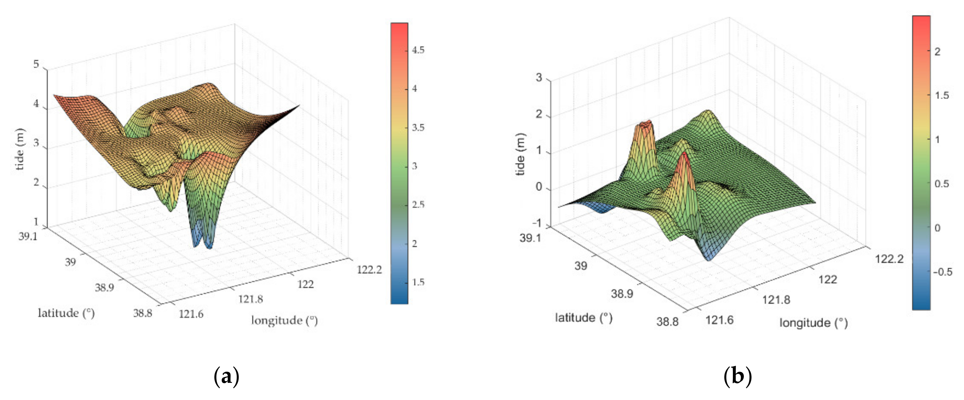
Calculate the distance between each measuring point. The gaussian model is used as a variation function to obtain . Finally, use Equation (1) to calculate the tide level of each point. The interpolation results obtained using the tide level value at high tide and low tide of Dalian Port are shown in Figure 6a, representing the interpolation tide level at high tide, and Figure 6b represents the interpolation tide level at low tide.

Figure 6.
(a). The interpolated tide level at high tide. (b). The interpolated tide level at low tide.
3.2.3. Wind Data
The immediate cause of the wind is the non-uniform distribution of air pressure in the horizontal direction due to the uneven temperature of the sea surface. Air flows from high pressure to low pressure. When the ship is sailing on the ocean, it will be affected by the force and moment of the wind, which will cause the ship to tilt, drift, and even stall. Therefore, the wind is one of the disturbance factors considered in ship motion modeling.
In calculating the wind load, the wind speed should be determined first. The wind speed at an average sea level of 10 m should be selected. For the static USV, the force and moment produced by the wind load on 3DOF can be obtained using the incompressible Bernoulli Equation (5) [29]. The correlation coefficients are shown in Table 3.
Table 3.
Correlation coefficients of the Bernoulli equation.
3.2.4. Current Data
Ocean currents refer to the large-scale movement of seawater caused by changes in temperature, salinity, and density between different water qualities or by wind friction. They are essential physical phenomena in the marine environment. Current can be divided into constant current, non-uniform current, steady current, and unsteady current according to the location and time characteristics. It needs complex theoretical derivation and many statistical experiments to be carried out on the uneven flow mathematical modeling. To simplify the current model in this paper, assume that the speed of the current change is not too great and sharp. Without loss of generality, the currents are supposed to be steady and uniform.
The force and moment of ocean current at USV with 3DOF are given:
where is the standard seawater density. is the acting force coefficient and acting moment coefficient of ocean current, which are generally obtained by experiment or system identification. is the projected area of the ship’s horizontal and longitudinal axes below the waterline and is the relative velocity of the current:
where and are the horizontal and longitudinal components of the relative current velocity. is the absolute current velocity and is the absolute current direction.
3.3. USV Dynamic Model
The dynamic model of the USV should be established first to analyze the force of its motion in 3DOF. The forces and moments suffered by the USV include thrusters, hydrodynamic forces, and moments, and marine environmental interference forces. Assuming that its center of gravity is located at the mid-longitudinal section, the differential equation of the USV hydrodynamic model is obtained as follows:
where is the symmetric positive definite inertia matrix, which is related to the ship’s linear velocity and angular acceleration:
is the centripetal and Coriolis matrix, depending on the additional mass of the USV:
is the damping coefficient matrix:
The environmental load can be divided into wind load and sea current load and can be expressed as:
3.4. USV Energy Consumption Model
The USV travels at a speed of at sea, and doing work to overcome the ocean environment consumes some of its energy. This paper substituted the mathematical Equations (5) and (6) into the linear dynamics model (9) to construct the total energy consumption model of the USV. Assuming that the gravity center of the USV is at the body-fixed coordinate system., the forces and moment provided by the propeller can be obtained when the USV moves with 3DOF as follows:
where represents the thrust of 3DOF. The dynamic parameters related to the above are shown in Table 4:
Table 4.
Hydrodynamic coefficient and parameters.
The energy consumption model of the USV under the wind and current can be obtained.
where , respectively, represents the energy consumption of the USV in the motion of sway, surge, and yaw from point to point . , respectively, represents the distance and heading angle of the USV in unit movement, and the calculation process is as follows:
The calculated energy consumption value is stored in the adjacency matrix , as shown in Table 5, is the energy consumption from point to , and is the energy consumption from point to . Note that and are not equal because the environmental data is a vector with different velocities in the opposite direction.
Table 5.
The node matrix J with energy consumption weight.
3.5. Dynamic Safe Water Depth Model
This section describes the generation principle of the dynamic Voronoi diagram. It includes three steps: the dynamic water depth model construction is introduced in Section 3.5.1, the Voronoi graph generation principle is introduced in Section 3.5.2, and the improved local Voronoi diagram is introduced in Section 3.5.3.
3.5.1. Dynamic Water Depth Generation
The dynamic water depth is calculated by the superposition of the water depth point and the interpolated tide:
where is the actual water depth of the point within one hour, is the water depth point extracted from the S-57 chart. is the tide of the point, and is the water depth change caused by other factors affecting the water level change of the point within one hour.
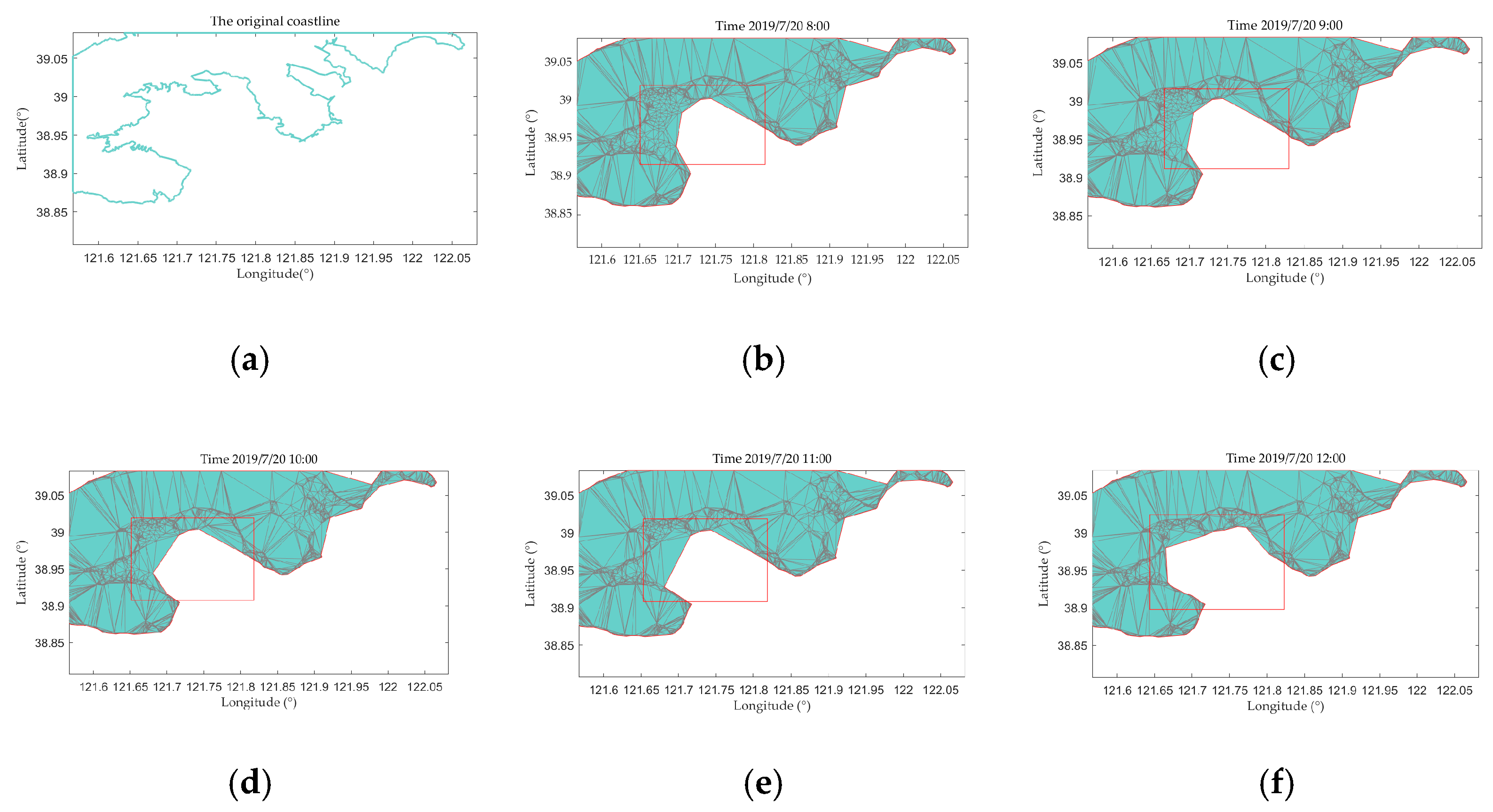
The minimum safe water depth is assumed to be 5 m, considering the performance of the USV and the tidal variation. Each hour’s dangerous water depth points are included in the obstacle set, applying the alpha shape algorithm to detect the edge points. Figure 7a is the initial coastline. Figure 7b–f is the model of safe water depth within five hours. It can be seen that the water depth does not change significantly in the first two hours. However, with the rise of tide level, the safe water depth area expands significantly, as marked in the rectangle.
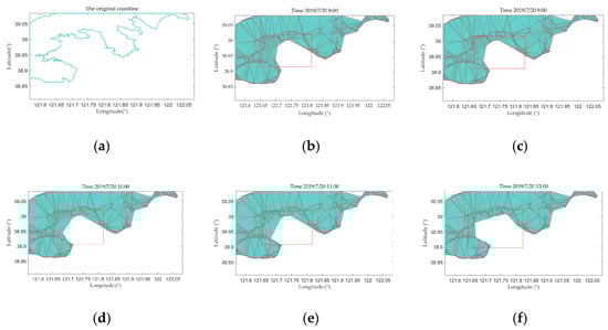
Figure 7.
Hourly safe water depth environment model: (a) represents the initial coastline; (b–f) represent a safe water depth environment model for five hours.
3.5.2. Voronoi Diagram Generation
The Voronoi diagram consists of a set of contiguous polygons. These edges are perpendicular bisectors of two adjacent points. It is widely used in geometry, architecture, geography, meteorology, and many other fields.
Suppose there exists a set containing points on the Euclidean plane , where . The Cartesian coordinates of these points are and do not overlap. The points are called sites, sorted from left to right and top to bottom, and connected to adjacent sites to form a convex hull triangulation network, as shown in Figure 8a. The Voronoi point is the center of the circumferential circle of each triangle. The connection of each Voronoi point is the Voronoi edge. They are stored in DCEL data structures. If is the point in Euclidean space and the coordinate is , then the distance between the point and another site is
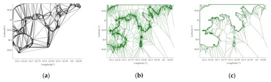
Figure 8.
Voronoi graph generation: (a) represents Delaunay triangulation; (b) represents the Voronoi roadmap. (c) Collision-free roadmap.
If is the nearest site or one of them, satisfies for any other point. The set of all qualified is called the original Voronoi region controlled by , and is expressed as:
As shown in Figure 8b, the set composed of all site control areas is defined as the original Voronoi diagram:
The dividing line of the area controlled by two different sites is a vertical bisector perpendicular to the connection line and , dividing the plane into two parts. Points within each site’s control area are less distant from that point than from the other site. Therefore, Voronoi modeling can maximize the use of gaps between obstacles so that the maximum distance of the route is far away from the obstacle, ensuring navigation safety.
The Voronoi diagram used for path planning environment modeling needs to be further improved and optimized. The Voronoi edge passing through the obstacle area needs to be deleted. First, delete all Voronoi edges connected to the Voronoi point set in the obstacle area. Then, judge whether there are still Voronoi edges passing through the obstacle area. If so, delete the edge and obtain the collision-free Voronoi diagram, as shown in Figure 8c.
Finally, vertices of Voronoi graphs that meet navigation requirements are stored in an adjacency matrix of , which stores the connection information of navigable edges. Assuming that vertex and vertex are connected, the adjacency matrices and are set to 1, as shown in Table 6. Otherwise, infinity Inf is set. The diagonal of the matrix is set to 0.
Table 6.
The node matrix .
3.5.3. Improved Voronoi Diagram Algorithm
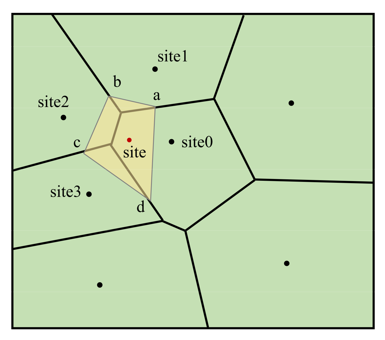
The safe water depth area is dynamically updated according to the tide data, and the Voronoi diagram also needs to be updated. However, regenerating the global Voronoi diagram will undoubtedly cause computational redundancy. Therefore, this paper adopts an incremental approach to construct a new cell. As shown in Figure 9, the new site is now inserted into the original Voronoi diagram. First, find the cell where the insertion site is located in the DCEL data structure. Connect the insertion site to Site0 and make a vertical bisector at points and . Transition to the cell region where the two intersections are located and use the same method to obtain and until the closed polygon is formed, creating the cell region belonging to the site, as shown in the yellow region:
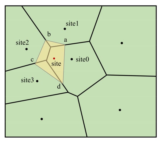
Figure 9.
The improved Voronoi diagram algorithm. a, b, c and d represent the intersection of the new Voronoi cell with the original Voronoi edge.
3.6. Voronoi Energy-Efficient Path Generation
The energy-efficient path planning algorithm based on the Voronoi diagram consists of the following three parts: setting timing breakpoint, an improved A* algorithm, and a new path optimization algorithm.
3.6.1. Set Timing Breakpoints
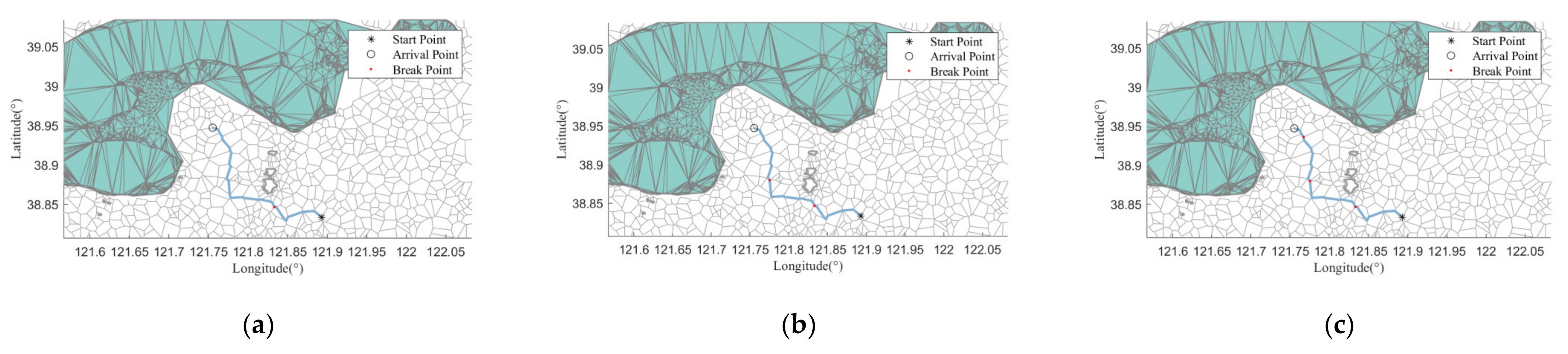
Marine environmental data for this paper are updated hourly, by setting timing breakpoints for the originally generated path based on the update time. As shown in Figure 10, the blue line represents the initially generated energy consumption path by the improved A* algorithm. The red dots represent the timing breakpoints. Figure 10a represents the timing breakpoint of the first hour, and Figure 10b represents the timing breakpoints of the second hour. Figure 10c represents the timing breakpoints of the third hour. When the USV navigates to the timing breakpoint of the first hour, it updates the marine environment data (using the data in the second hour) to plan a dynamic energy-efficient path.
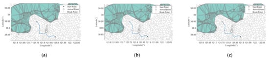
Figure 10.
The breakpoint of a minimal energy-consuming path. (a) The breakpoint for the first hour. (b) The breakpoint for the second hour. (c) The breakpoint for the third hour.
Setting a timing breakpoint that is dynamically updated by marine environmental data can be considered, which is more conducive to the USV navigating for a long time at sea.
3.6.2. The Improved A* Search Algorithm
The cost function of the traditional A* algorithm is composed of the actual cost function and heuristic function, which can search for the shortest path quickly and effectively. In this paper, the traditional A* algorithm is improved to replan the energy-efficient path considering the distance under wind and current influence. The actual cost function evaluates the energy consumption of the path, and the heuristic function evaluates the shortest distance of the path. This path planning with comprehensive consideration of energy consumption and distance can be obtained. The cost function of the A* algorithm is:
where is the energy consumption function from the initial point to the middle point. is the heuristic function, defined as the distance between the middle and the arrival points. The calculation of the distance:
The energy consumption and heuristic functions are normalized to obtain dimensionless data, convenient for subsequent operations. The improved A* algorithm pseudocode is as followed (Algorithm 1):
| Algorithm 1: The improved A* algorithm pseudocode |
| Function path=A_star(START, GOAL, J) |
| f(xc) ← inf // f(xc) = e(xc) + h(xc) is a total cost of current node xc, where e(xc) is an energy consumption from START to xc and h(xc) is a heuristic cost form xc to GOAL. |
| START ∈ OPEN |
| While OPEN is not empty |
| ifxc = GOAL |
| Break |
| end |
| xc ∈ CLOSED |
| for each neighbor xv of xc |
| ifxv ∉ CLOSED |
| Cost(xv) ← e(xc) + Cost(xv)//the edge cost of xv |
| ifxv ∉ OPEN && Cost (xc) < e(xv) |
| e(xv) ← Cost(xc) |
| h(xv) ← heuristic cost of xv |
| f(xv) ← e(xv) + h(xv) |
| Parent(xv) ← xc |
| ifxv ∈ OPEN |
| OPEN. remove(xv) |
| end |
| end |
| end |
| end |
| path ← Parent(path)//path is generated by connecting the parent nodes starting from GOAL note. |
| end |
3.6.3. The Path Optimization Algorithm
Although the number of navigable paths is increased by constructing the Voronoi diagram with discrete, safe water depth points, it also causes many inflection points and uneven paths, which do not meet the requirements of sea navigation. Therefore, the generated energy-efficient path will be smoothly optimized.
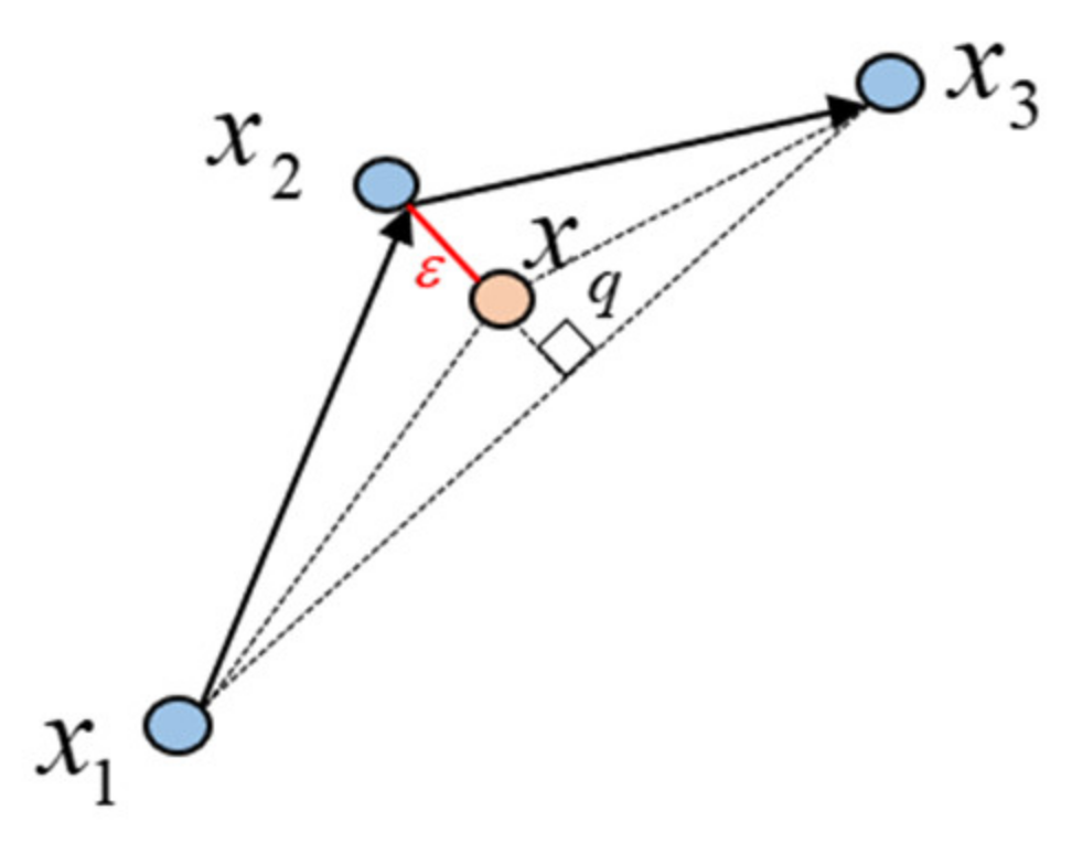
Traditional optimization algorithms cannot be used to optimize the path because of the lower energy consumption of the initial energy-efficient path. These algorithms will cause the problem that the optimized path still consumes much energy. As shown in Figure 11, it is assumed that the USV will sail from node to node through a turning point . First, calculate whether the distance between the middle node and the two nodes exceeds the preset threshold . If the distance does not exceed the threshold, delete nodes and directly connect the first and last nodes to form a new path. If the threshold is exceeded, move the intermediate node to with the distance of . Reconnect node , node , and node again to create a new path.
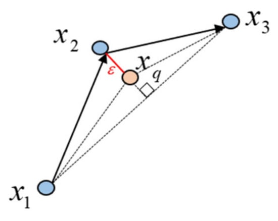
Figure 11.
The path optimization algorithm.
As shown in Figure 12a, the blue line represents the path before optimization, and the number of nodes is 41. The black line represents the optimized path, and the number of nodes is 21. The number of nodes is reduced by 50%. However, the turning angle still does not meet the requirements of precise navigation maneuvering. The paper applies a uniform B-spline curve to smooth the steering angle, and the B-spline curve equation can be written as:
where is the coordinate of a path node, is the standard B-spline basis function of degrees, and the highest degree is . The Cox-de Boor recursive equation is usually adopted:
where is the node serial number and is the node vector, which can be generated by using the function of Matlab. Set to obtain the path as shown in Figure 12b. The blue dots represent the waypoints. The orange line represents the final path after optimization, indicating that the smoothness has been improved.
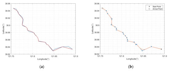
Figure 12.
Path smoothing effect. (a) Comparison between waypoint and before optimization. The blue line represents the path before optimization, and the red line represents the optimized path. (b) The action of the B-spline curve. The blue dots represent the waypoints and the orange line represents the final path after optimization.
4. Simulation Results and Discussion
To verify the effectiveness of the proposed energy-efficient path planning algorithm, simulation experiments are carried out on Matlab2019 (Windows10, Intel (R) Core (TM) i7-10710u CPU @ 1.10 GHz 1.61 GHz, memory 16 G). Firstly, the start point (121.8929, 38.8334) and the arrival point (121.7552, 38.9470) are set. The basic parameters of the USV are shown in Table 7. The original current and wind data are shown in Table 1 and Table 2. After interpolation, the average current velocity of Dalian Bay is 2m/s; the average wind speed is 7m/s. The wind and current direction are mainly east and south. The tidal data were collected from 8:00 to 12:00 on 20 July 2019.
Table 7.
Basic parameters of USV.
4.1. Energy Saved in Favorable Situation and Counter Situation
This section analyzes the energy saved of the minimal energy-consuming path (the E path) in favorable and counter situations and does not consider the variation of ocean data and distance costs. Set the speed of the USV to 2.1 m/s. The E path and the shortest path are obtained, respectively, in favorable and counter situations, and the data are shown in Table 8.
Table 8.
The data of the minimal energy-consuming path and the shortest path in favorable and counter situations.
Figure 13a,b represents the E path and the shortest path under a favorable situation. The E path automatically plans the voyage to the place where the wind and currents are weak. Figure 14c shows both paths’ energy consumption over time under favorable conditions. The shortest path consumes a short time, but the energy distribution is very concentrated. Although the distance and planning time of the E path is longer than the shortest path, the energy efficiency is increased by 27%. In Figure 14d,e, switch the start and arrival points to generate the E path and the shortest path under the contour situation. The E path consumes 499.63 kJ of energy, while the shortest path consumes 560.27 kJ of energy. The energy saved is only 11%, which is much lower than favorable conditions. Because the relative wind and current speed are low in a favorable situation, the energy consumption is relatively low; therefore, the USV can best use favorable current and wind. However, as is shown in Figure 14f, the energy consumption of the E path is higher in a counter situation, which is not much different from the energy consumed by the shortest path.
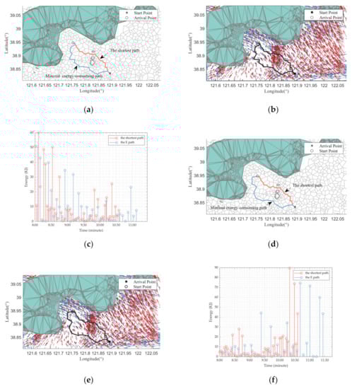
Figure 13.
Comparison between the minimal energy-consuming path and the shortest path. (a,b) Comparison between the minimal energy-consuming path and the shortest path in a favorable situation. (c) represents the energy consumption over time in a favorable situation. (d,e) Comparison between the minimal energy-consuming path and the shortest path under a counter situation. (f) represents the energy consumption over time in a contour situation.
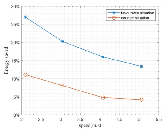
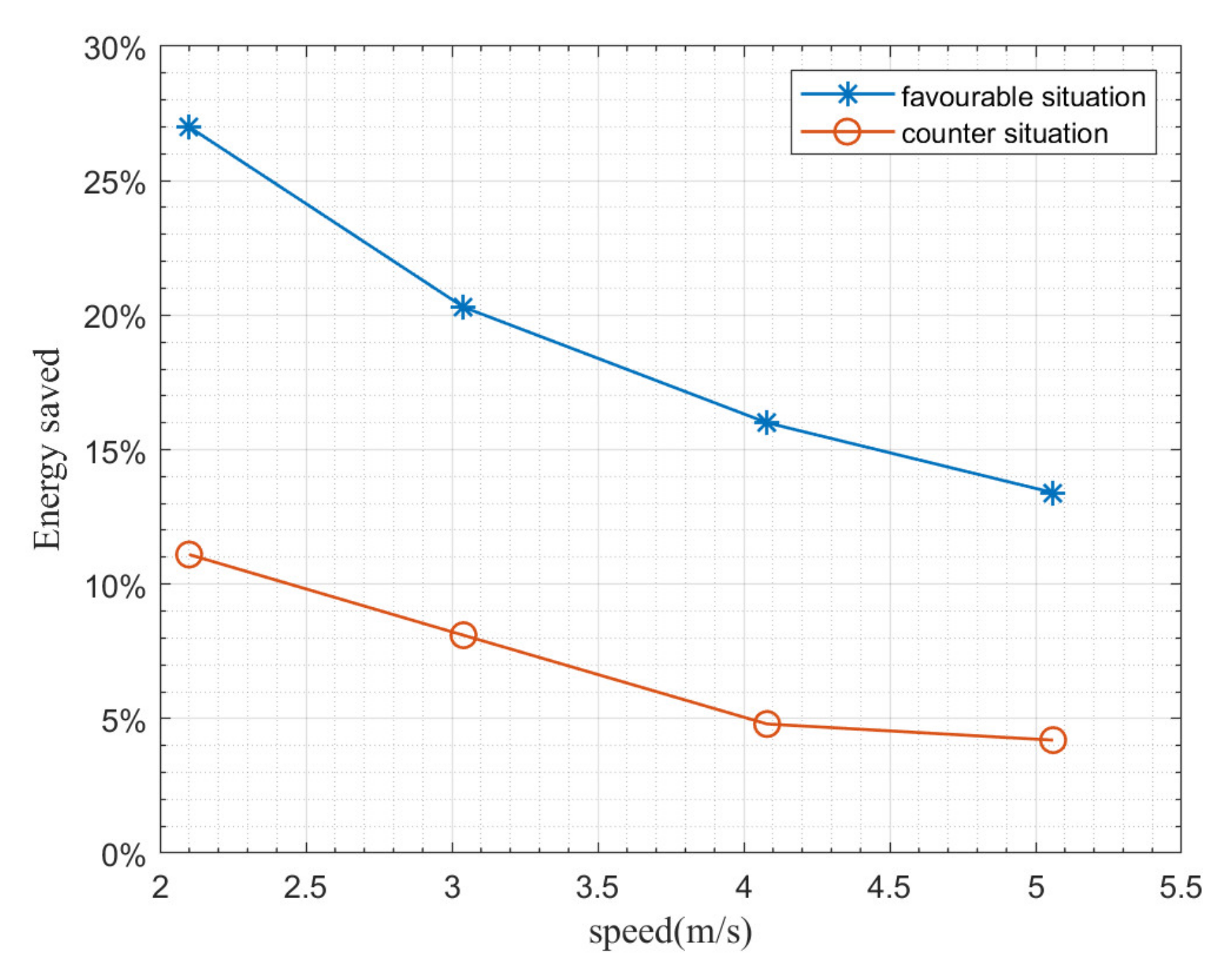
Figure 14.
The energy-saving rate at different speeds of USV under different situations.
4.2. Energy Saved at Different Speeds of USV
USVs encounter different environmental resistance and consume different energy when sailing at different speeds. To study the energy consumption of the USV at different speeds, the speed of the USV is set as 2.1 m/s, 3.04 m/s, 4.08 m/s, and 5.05 m/s, respectively. Simulations in different situations analyze the energy-saving rate of the E path. The simulation results are shown in Figure 14. The blue line represents the energy-saving rate under favorable conditions, and the red line represents the energy-saving rate under counter conditions. As the USV speed increases, so does the static water resistance. More energy is required to overcome static water resistance. Meanwhile, the energy-saving rate of favorable situations is higher than that of counter conditions, which is further verified by 4.1.
4.3. Dynamic Energy-Efficient Path Planning Considers the Distance
4.3.1. Comparison between the Dynamic ED Path and the Shortest Path
The USV is affected by time-varying environmental factors when it sails for a long time. To analyze the influence of wind, current, and tide in each time bucket, this paper planned an hourly dynamic energy-efficient path that considered the distance between the start point (121.8929, 38.8334) and the arrival point (121.7552, 38.9470).
Set the USV speed to constant 2.1m/s. The path is divided into four-time segments. The energy-efficient path is constructed based on the environment information in each time segment. Firstly, the dynamic, safe water depth model needs to be built according to the tide data. Extract water depth points less than 5 m and put them into the coastline set to build the dynamic, safe water depth model using the improved Voronoi diagram algorithm. Figure 7 of Section 3.5.1 shows that the tide does not change much during the first two hours. Thus, the environment model for the first hour is approximated to replace the previous two hours. Secondly, set a timing breakpoint based on the initial path, already mentioned in Section 3.6.1.
Finally, combined with each hour’s wind and current data (assuming that when the USV enters the second-hour voyage planning, the wind and current data of the second hour shall be used for replanning), the dynamic energy-efficient path considers the distance (the dynamic ED path) generated by applying the improved A* algorithm, shown as the blue line in Figure 15a. The red line represents the hourly dynamic minimal energy-consuming path (the dynamic E path). The dynamic ED path saves energy and shortens the overall range compared to the dynamic E path. In Figure 15b, the blue line represents the dynamic ED path without timing breakpoints. The orange line represents the shortest path. The changes in energy consumption over time of the three paths are shown in Figure 15c. The dynamic E path consumes the most energy, while the dynamic ED path consumes the least energy.
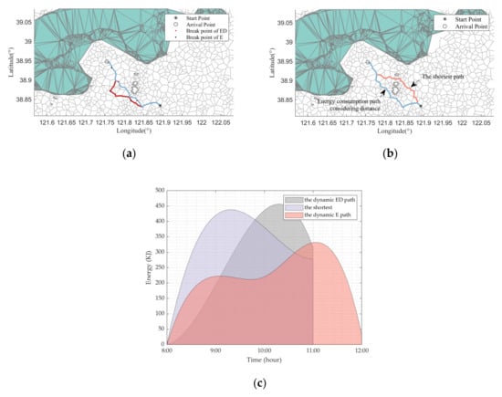
Figure 15.
(a) Comparison between hourly dynamic energy-efficient path considers the distance and hourly minimal energy-consuming path. (b) Comparison between hourly dynamic energy-efficient paths considers the distance and the shortest path; (c) represents the energy consumption over time of three paths.
Compared with the shortest path, the energy consumption per hour is shown in Table 9. The total range of the dynamic ED path is 21,929 m. The shortest path is 21,390 m. The dynamic E path has a range of 22,976.9 m. The energy-saving rate of the dynamic E path is 25% higher than that of the shortest path, however, it takes a longer time. The energy saved depends on the relative wind speed and current velocity of the extra time, so the energy saved may be very low or even harmful. Therefore, the cost of the distance must be considered when planning an energy-efficient path. Compared with the shortest path, the total voyage of the dynamic ED path has little change and the energy-saving rate increases by 12%. The result of planning has a more practical application value.
Table 9.
Comparison of hourly dynamic energy-efficient path considers the distance, the shortest path, and hourly minimal energy-consuming path.
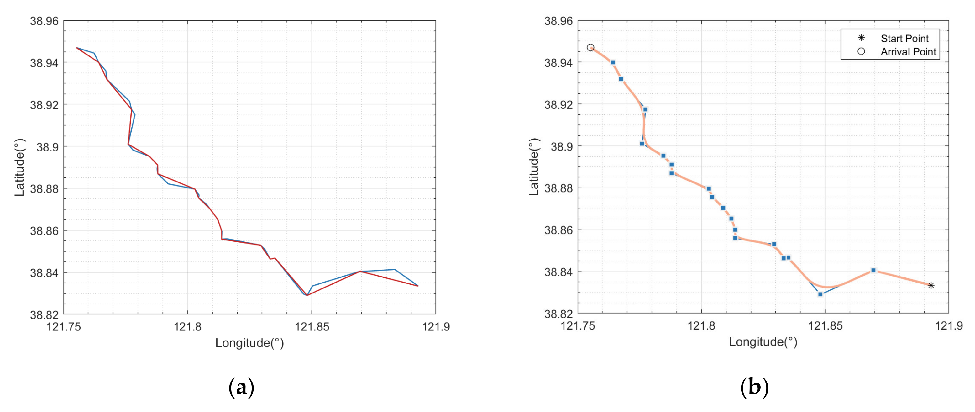
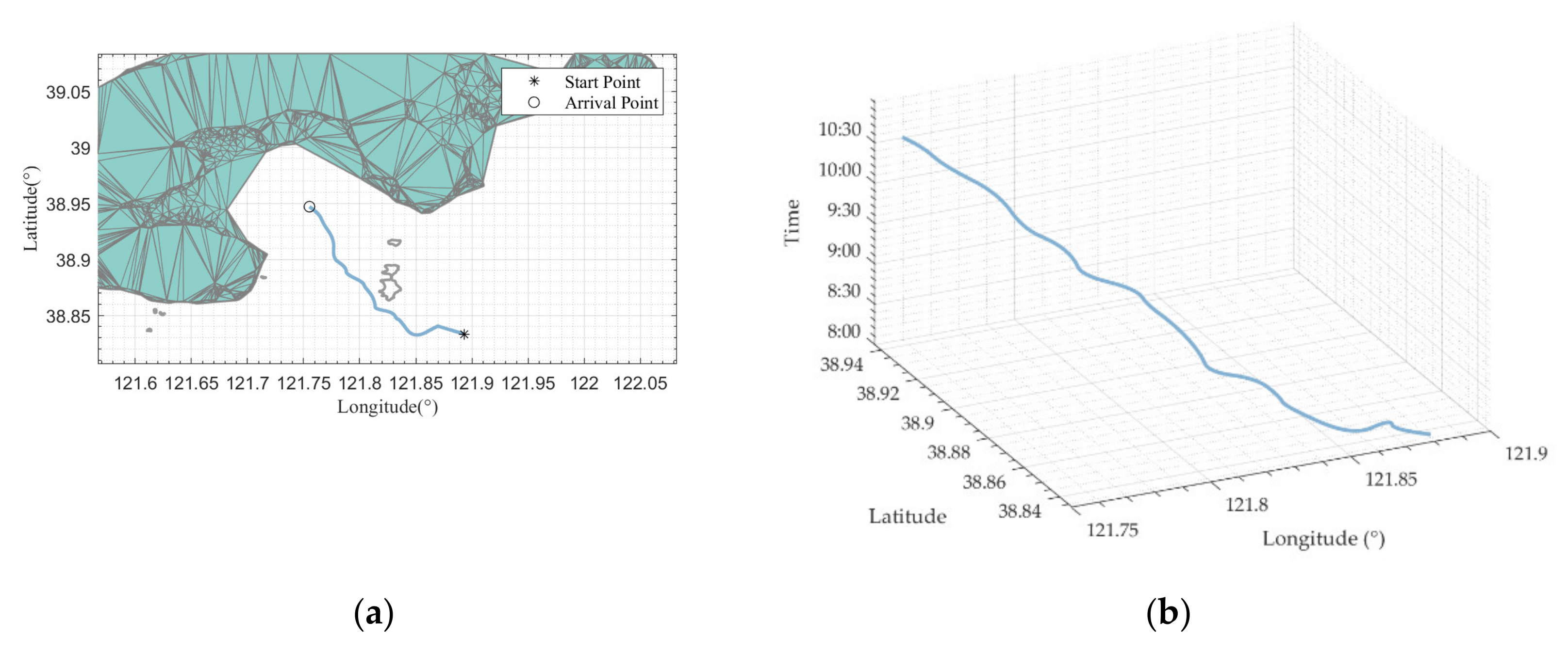
Finally, the dynamic ED is optimized. The number of waypoints before the optimization is 41, and the number after optimization is 21, significantly reducing the number of waypoints. Meanwhile, the turning angle of each waypoint is optimized to obtain the final dynamic energy-efficient path considering the distance, as shown in Figure 16a. Figure 16b shows the relationship between position and time of the USV, including latitude and longitude coordinates and the steering angle. It can be seen from the simulation results that the steering change is reasonable when it advances to the arrival point. The target was reached in two and a half hours, taking into account time-varying ocean data.
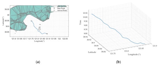
Figure 16.
Where (a) represents the hourly dynamic energy-efficient path and considers the distance after optimization. (b) Simulation results of positions of USV concerning time.
The mission of changing voyage is shown in Table 10. In mission 4, the USV voyage can be demonstrated under cross-wind and cross-current. The energy-saving rate is lower than that under the favorable situation in mission 1, showing that the greater the interference of the external environment, the greater the energy consumption and the lower the energy-saving rate of the USV.
Table 10.
Comparison of hourly dynamic energy-efficient path considers the distance and the shortest path.
4.3.2. Comparision between the Dynamic ED Path and the VVEE Path
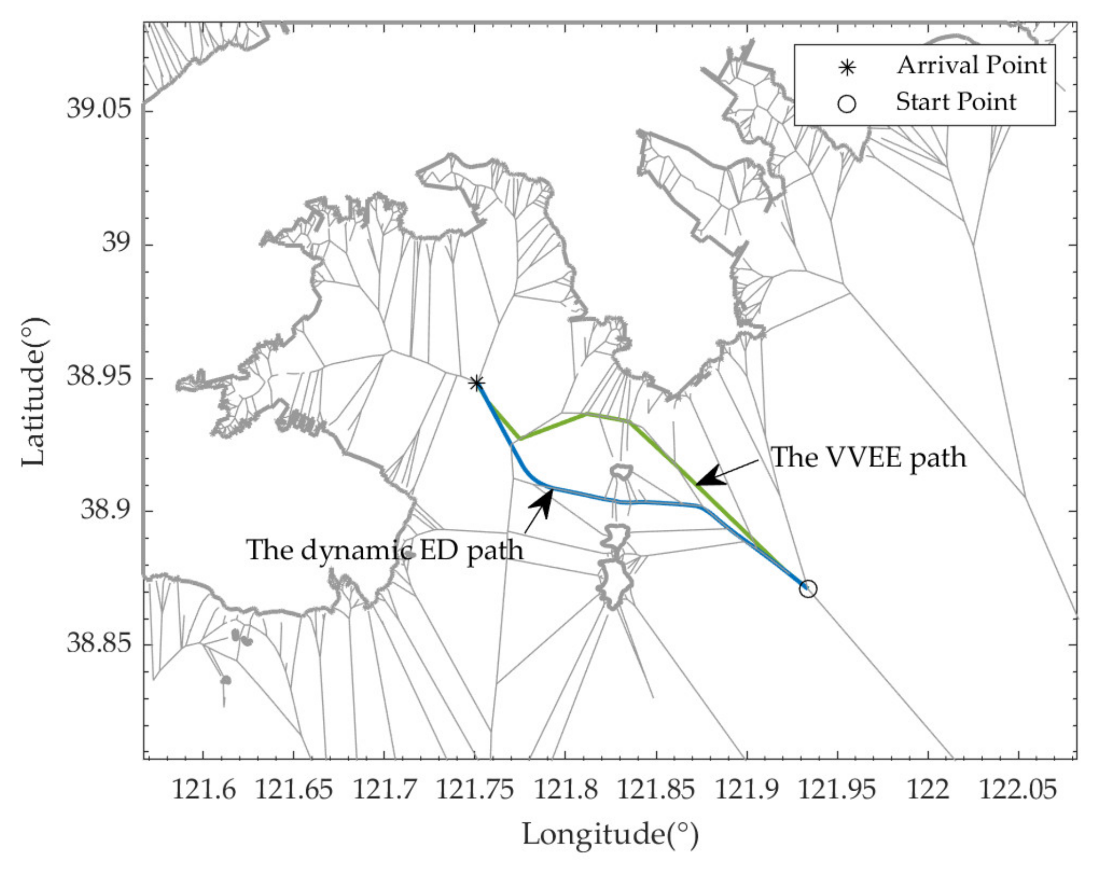
The dynamic ED path is compared and analyzed with the VVEE algorithm proposed in reference [10] to verify the algorithm’s effectiveness in this paper. The VVEE algorithm only considers the effect of ocean currents. This paper will compare the energy and path length consumed by the two algorithms under the influence of ocean currents and the constraints on USV motion. Furthermore, with setting the same size data set, the simulation result is shown in Figure 17. The blue line represents The dynamic ED path proposed in this paper. The green line represents the VVEE path. The simulation data is listed in Table 11. It is found that the dynamic ED path increases by 37% compared with the VVEE path in terms of energy consumption. The VVEE path uses favorable ocean currents and dramatically reduces energy consumption. However, The dynamic ED path proposed in this paper considers the current variation and distance cost, which shortens by 9% and is more consistent with the actual application situation. As the current velocity increases over time, the energy consumption of the dynamic ED path increases. These two algorithms are excellent in terms of time. The path can be successfully planned for the next few hours in seconds. It can be seen that these two algorithms are suitable for large data set operations.
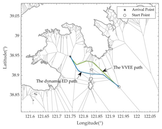
Figure 17.
Comparison between the dynamic ED path and the VVEE path.
Table 11.
Comparison between the dynamic ED path and the VVEE path.
The VVEE algorithm has fewer constraints than the proposed algorithm in this paper. The algorithm in this paper considers wind, current, and tide changes based on the VVEE algorithm. The stress of 3DOF for the USV is analyzed. The A* algorithm is improved to obtain the energy-efficient path that considers the distance, which is more in line with the navigation needs.
5. Conclusions
Based on measured marine environmental information, an hourly dynamic energy-efficient path considering the distance is proposed, which mainly includes the following parts:
- Extract coastline coordinates and static water depth data from the S-57 electronic chart, using the Voronoi diagram to build a model that conforms to the natural navigation environment.
- The dynamic, safe water depth model is constructed using the improved Voronoi diagram after superposing the interpolated tide data with the static water depth data.
- The influence of wind and currents on the USV during the operation period should be fully considered. The total energy consumption model is constructed by combining the mathematical models of wind and current and the dynamics model of the USV.
- The time breakpoints are planned according to the distance of the general mission to consider the time-varying wind and current. The improved A* algorithm replicates the path according to the timing breakpoint. The dynamic energy-efficient path considers the distance obtained.
- This paper proposes a new optimization algorithm for the dynamic energy-efficient path that considers the distance to reduce the number of waypoints and smooth the path.
According to the simulation results, the following conclusions are drawn:
- A comparative analysis is made between the minimal energy-consuming path and the shortest path in a favorable situation without considering the distance. The minimal energy-consuming path takes advantage of a friendly environment to reduce energy consumption to the greatest extent. However, the distance cost is relatively high. In the counter situation, the difference in energy consumption between the minimal energy-consuming path and the shortest path is slight. The relative wind speed and current velocity in the counter situation are significant, resulting in a low energy- saving rate.
- Secondly, the energy-saving rate of the minimal energy-consuming path under different speeds is analyzed. In any marine environment, the higher the speed, the lower the energy efficiency. Because of the significance of the static water resistance of the USV at high speed, the more work it does to overcome static water resistance. The greater the energy consumption, the lower the corresponding energy-saving rate. In addition, compared with the counter situation, more energy can be saved, and the energy-saving rate is higher in a favorable situation.
- This paper defines time breakpoints for path replanning to obtain an hourly dynamic energy-efficient path that considers the distance and the shortest path. Under the premise that the planning of the distance is similar, the energy-saving rate increases by 12%. Although the energy-saving rate is not as high as the minimal energy-consuming path, this paper comprehensively considers the distance and energy consumption factors. It is more in line with the actual navigation requirements.
- The analyzed dynamic energy-efficient path considers the distance and the shortest path under different speeds. It was found that the higher the speed, the more decreased the energy-saving rate.
- It also increases the energy-saving rate under cross-wind and cross-flow, which is still lower than that under a favorable situation.
- The proposed method is compared with another method in energy consumption, planning time, and path length. The energy consumption of the proposed method is higher than that of another method because the current variation and path length cost is considered. In addition, it performs better in planning time and has short distances. In addition, the proposed algorithm can take marine environmental changes into more comprehensive consideration. It is necessary to plan a dynamic energy-efficient path on a long voyage, which can improve the endurance of the USV and save a lot of energy consumption.
This paper briefly discusses energy-efficient path planning under the influence of wind and current. However, there are still the following problems: it is roughly assumed that the wind, current, and tide change by the hour, which does not achieve dynamic planning in an absolute sense. Apart from that, the impact of waves on the hull needs to be considered. Due to the lack of experimental conditions, there is no physics experiment result verification. Further research will be carried out on the above issues in the future.
Author Contributions
Conceptualization, Y.Z. and G.S.; methodology, Y.Z.; software, Y.Z.; validation, Y.Z. and J.L.; formal analysis, Y.Z.; investigation, Y.Z.; resources, Y.Z.; data curation, Y.Z.; writing—original draft preparation, Y.Z.; writing—review and editing, Y.Z.; visualization, Y.Z.; supervision, G.S.; project administration, G.S.; funding acquisition, G.S. All authors have read and agreed to the published version of the manuscript.
Funding
This research was funded by the Fundamental Research Funds for the Central Universities, the funding number 3132022157.
Institutional Review Board Statement
Not applicable.
Informed Consent Statement
Not applicable.
Data Availability Statement
The data that support the findings of this study are available within the article.
Acknowledgments
We are especially grateful to the Navigation Safety Guarantee Institute for its financial and technical support.
Conflicts of Interest
The authors declare no conflict of interest.
References
- Peng, Y.; Yang, Y.; Cui, J. Development of the USV ‘JingHai-I’ and sea trials in the Southern Yellow Sea. Ocean Eng. 2017, 131, 186–196. [Google Scholar] [CrossRef]
- Liu, Z.; Zhang, Y.; Yu, X. Unmanned surface vehicles: An overview of developments and challenges. Annu. Rev. Control 2016, 41, 71–93. [Google Scholar] [CrossRef]
- He, S.; Wang, M.; Dai, S.L. Leader-Follower Formation Control of USVs with Prescribed Performance and Collision Avoidance. IEEE Trans. Ind. Inform. 2018, 15, 572–581. [Google Scholar] [CrossRef]
- Zhou, C.; Gu, S.; Wen, Y. The Review Unmanned Surface Vehicle Path Planning: Based on Multi-modality Constraint. Ocean Eng. 2020, 200, 1873–5258. [Google Scholar] [CrossRef]
- Campbell, S.; Naeem, W.; Irwin, G.W. A review on improving the autonomy of unmanned surface vehicles through intelligent collision avoidance manoeuvres. Annu. Rev. Control 2012, 36, 267–283. [Google Scholar] [CrossRef] [Green Version]
- Yang, J.M.; Tseng, C.M.; Tseng, P.S. Path planning on satellite images for unmanned surface vehicles. Int. J. Nav. Archit. Ocean Eng. 2015, 7, 87–99. [Google Scholar] [CrossRef] [Green Version]
- Xie, L.; Xue, S.; Zhang, J. A path planning approach based on multi-direction A* algorithm for ships navigating within wind farm waters. Ocean Eng. 2019, 184, 311–322. [Google Scholar] [CrossRef]
- Lee, T.; Kim, H.; Chung, H. Energy efficient path planning for a marine surface vehicle considering heading angle. Ocean Eng. 2015, 107, 118–131. [Google Scholar] [CrossRef]
- Niu, H.; Savvaris, A.; Tsourdos, A. Voronoi-Visibility Roadmap-based Path Planning Algorithm for Unmanned Surface Vehicles. J. Navig. 2019, 72, 850–874. [Google Scholar] [CrossRef]
- Niu, H.; Lu, Y.; Savvaris, A. An energy-efficient path planning algorithm for unmanned surface vehicles. Ocean Eng. 2018, 161, 308–321. [Google Scholar] [CrossRef] [Green Version]
- Dijkstra, E.W. A note on two problems in connexion with graphs. Numer. Math. 1959, 1, 269–271. [Google Scholar] [CrossRef] [Green Version]
- Hart, P.E.; Nilsson, N.J.; Raphael, B. A Formal Basis for the Heuristic Determination of Minimum Cost Paths. IEEE Trans. Syst. Sci. Cybern. 1972, 4, 100–107. [Google Scholar] [CrossRef]
- Garau, B.; Bonet, M.; Alvarez, A. Path Planning for Autonomous Underwater Vehicles in Realistic Oceanic Current Fields: Application to Gliders in the Western Mediterranean Sea. J. Marit. Res. 2009, 6, 5–22. [Google Scholar] [CrossRef]
- Dorigo, M.; Caro, G.D.; Gambardella, L.M. Ant Algorithms for Discrete Optimization. Artif. Life 1999, 5, 137–172. [Google Scholar] [CrossRef] [Green Version]
- Holland, J.H. Adaptation in Natural and Artificial Systems: An Introductory Analysis with Applications to Biology, Control and Artificial Intelligence; MIT Press: Cambridge, MA, USA, 1992; Volume 211. [Google Scholar]
- Kennedy, J.; Eberhart, R. Particle swarm optimization. In Proceedings of the ICNN’95—International Conference on Neural Networks, Perth, WA, Australia, 27 November–1 December 1995; Volume 4, pp. 1942–1948. [Google Scholar] [CrossRef]
- Liu, X.; Li, Y.; Zhang, J. Self-Adaptive Dynamic Obstacle Avoidance and Path Planning for USV Under Complex Maritime Environment. IEEE Access 2019, 7, 114945–114954. [Google Scholar] [CrossRef]
- Ding, F.; Zhang, Z. Energy-efficient Path Planning and Control Approach of USV Based on Particle Swarm optimization. In Proceedings of the OCEANS 2018 MTS/IEEE, Charleston, SC, USA, 22–25 October 2018; pp. 1–6. [Google Scholar] [CrossRef]
- Lavalle, S.M. Rapidly-Exploring Random Trees: A New Tool for Path Planning, Research Report. Available online: http://msl.cs.illinois.edu/~lavalle/papers/Lav98c.pdf (accessed on 5 March 2022).
- Kamarry, S.; Molina, L. Compact RRT: A New Approach for Guided Sampling Applied to Environment Representation and Path Planning in Mobile Robotics. In Proceedings of the 2015 12th Latin American Robotics Symposium and 2015 3rd Brazilian Symposium on Robotics (LARS-SBR), Uberlândia, Brazil, 28 October–1 November 2015; pp. 259–264. [Google Scholar] [CrossRef]
- Wang, Y.; Liu, M. Semantical obstacle representation model for fast UAV path planning. In Proceedings of the 2017 2nd Asia-Pacific Conference on Intelligent Robot Systems (ACIRS), Wuhan, China, 16–18 June 2017; pp. 180–184. [Google Scholar] [CrossRef]
- Li, D.; Wang, X. Energy-optimal coverage path planning on topographic map for environment survey with unmanned aerial vehicles. Electron. Lett. 2016, 52, 699–701. [Google Scholar] [CrossRef]
- Subramani, D.N.; Lermusiaux, P. Energy-optimal path planning by stochastic dynamically orthogonal level-set optimization. Ocean Model. 2016, 100, 57–77. [Google Scholar] [CrossRef] [Green Version]
- Yu, H.; Wang, Y. Multi-objective AUV Path Planning in Large Complex Battlefield Environments. In Proceedings of the 2014 Seventh International Symposium on Computational Intelligence and Design, Washington, DC, USA, 13–14 December 2014; pp. 345–348. [Google Scholar] [CrossRef]
- Yilmaz, N.K.; Evangelinos, C.; Lermusiaux, P. Path Planning of Autonomous Underwater Vehicles for Adaptive Sampling Using Mixed Integer Linear Programming. IEEE J. Ocean. Eng. 2008, 33, 522–537. [Google Scholar] [CrossRef] [Green Version]
- Du, Z.; Wen, Y.; Xiao, C. Motion planning for Unmanned Surface Vehicle based on Trajectory Unit. Ocean Eng. 2018, 151, 46–56. [Google Scholar] [CrossRef]
- Vu, M.T.; Van, M.; Bui, D.H.P. Study on Dynamic Behavior of Unmanned Surface Vehicle-Linked Unmanned Underwater Vehicle System for Underwater Exploration. Sensors 2020, 20, 1329. [Google Scholar] [CrossRef] [Green Version]
- Nguyen, X.T.; Nguyen, B.T.; Do, K.P. Spatial Interpolation of Meteorologic Variables in Vietnam using the Kriging Method. J. Inf. Processing Syst. 2015, 11, 134–147. [Google Scholar] [CrossRef]
- Gu, S.; Zhou, C.; Wen, Y. Motion Planning for an Unmanned Surface Vehicle with Wind and Current Effects. J. Mar. Sci. Eng. 2022, 10, 420. [Google Scholar] [CrossRef]


Publisher’s Note: MDPI stays neutral with regard to jurisdictional claims in published maps and institutional affiliations. |
© 2022 by the authors. Licensee MDPI, Basel, Switzerland. This article is an open access article distributed under the terms and conditions of the Creative Commons Attribution (CC BY) license (https://creativecommons.org/licenses/by/4.0/).