A Novel Analytical Solution Method for Celestial Positioning

Abstract

Traditional celestial navigation adopts the intercept method or Sumner line method in order to solve the fix problems of celestial sight reduction. While an estimated position is often needed in order to complete celestial positioning, these methods are not rigorous and they have many shortcomings. Thus, this study has analyzed the geometry of the circle of equal altitude and the two-body problem. Furthermore, vector methods are proposed without using spherical trigonometry, in order to meet navigation needs. Finally, web mapping was used to display the results. The results show that the two methods that are proposed in this study had better accuracy, practical convenience, and faster computing speed than those which have been proposed by other studies. The two methods’ capability to avoid complicated manual calculations and chart work processes makes them highly suitable as an alternative to the use of global navigation satellite systems. These methods enable maritime school students to quickly understand the principles of celestial navigation through computing and graphical interfaces.

1. Introduction

Traditional celestial navigation uses a marine sextant in order to observe and obtain the altitude of celestial bodies above the horizon, such as the Sun, the Moon, planets, and stars. After measuring the altitude of a celestial body, the navigator can obtain the circle of equal altitude that is passing through the navigator’s ship’s position. In addition, the circle of equal altitude, also called the circle of position (CoP), is the real line of position in celestial navigation. However, the most possible position can only be calculated by observing at least two celestial bodies. The CoP is a small circle [1,2,3]. On the other hand, in geographic information systems (GIS), the feature layers include three forms: points, lines, and polygons; which also constitute the range of the vector data. Celestial positioning is one of the applications of small circles and it belongs to the polygonal feature. These can be extended to navigation applications and research, such as location-based services (LBS), radar range rings, and guard zones. This study was developed based on the concept of small circles.

In previous literature, researchers have used the closed analytic solution in order to solve the two-star sight problem of celestial positioning [4]. Some researchers have adopted simultaneous equations [5], while others have acquired the position by calculating the two intersections of two small circles using the vector method and the spherical triangle method [6,7]. Furthermore, the genetic algorithm (GA) and particle swarm optimization were also applied for the first time in calculating the mathematical optimization of celestial positioning [8,9]. The Sumner line method, as proposed by US Navy Captain Thomas Hubbard Sumner, has been explored by a small number of researchers [10,11]. It is noteworthy that the related abovementioned literature has adopted either two- or multi-body fixes. Considering that there are often restrictions in choosing celestial bodies and the time that is needed to observe them in practice, the two-body fix is generally a more favorable option for seafarers.

With today’s highly developed technology, GNSS is essential to seafarers. When performing ocean navigation, GNSS provides a continuous real-time fix and, when combined with an electronic chart and display information system (ECDIS), unlimited availability and convenience are made feasible. Although electronic navigation aids have been developed continuously, the education of celestial navigation is still being promoted. In Section B-II/1 of the 2010 Manila amendments of the International Convention on Standards of Training, Certification, and Watchkeeping for Seafarers (STCW) it is mentioned that seafarers must be able to not only practice celestial positioning and adjust compass errors accordingly but also use Electronic Nautical Almanac and celestial navigation calculation software [12]. Therefore, celestial navigation still plays an irreplaceable role in contemporary navigation education.

This study has applied the system linear equation to celestial positioning and divided it into Newton’s method and the closed analytical solution method in order to complete the solution. The linear equation system is quite common and no complicated optimization algorithms, such as ant colony optimization (ACO), are required. The main tools that were used in this paper were the MATLAB^® (Natick, MA, USA) and MAPLE^® (Waterloo, ON, Canada) computer algebra system programs. These programs are easy to operate and can help users to derive the algorithms and equations that are necessary to solve celestial positioning problems. Moreover, an HTML-based user-friendly graphical user interface (GUI) was designed and the algorithm was embedded into JavaScript^® (Austin, TX, USA) code so as to present the results of the celestial positioning with web mapping [13]. The figures in this paper were drawn using the geospatial data (kml and kmz) that had been input into Google Earth. The proposed system could allow students of maritime schools to learn the principles of celestial positioning more simply and clearly.

2. The Theoretical Foundation of Solving the Intersection of Two CoPs in Celestial Positioning

Traditionally, navigators have needed to obtain the celestial altitude of at least two celestial bodies with a marine sextant and then correct them using the Nautical Almanac so as to determine the observed altitude (Ho) of the celestial bodies. The co-altitude, also called the zenith distance (Zd), forms a CoP for each observation. In addition, the coordinates of the celestial bodies, such as the declination (Dec) and Greenwich hour angle (GHA), are projected onto the Earth and are known as geographic positions (GP). If the two celestial bodies are observed simultaneously (or nearly simultaneously), one of the two intersections of the two CoPs will be the vessel’s actual position. With the help of dead reckoning (DR), the estimated position (EP), or the assumed position (AP), it is possible to determine the correct position of the observer.

Due to the limitations of the traditional paper nautical chart scale, navigators use the intercept method (IM), also called the difference of altitude method or Marcq St. Hilaire method, to calculate their celestial positioning. This method was proposed in 1875 by the French navy officer Marcq de St. Hilaire (1832–1889) [2,5]. Navigators use the intercept method (IM) to obtain the tangent line of the CoP on the Mercator chart, also called the celestial line of position (LOP), as shown in Figure 1.

3. Celestial Sphere and Cartesian Coordinates System Conversion

The celestial sphere is considered to be a Cartesian coordinate system that is orthogonal, Earth-centered, and Earth-fixed (ECEF). The Cartesian coordinate system is a unit sphere with a radius of 1 [14,15,16], as shown in Figure 2 Vector P is the vessel’s position, as given by Equation (1).

$$P\left(lat,lng\right)=\left[\begin{array}{c}x\\ y\\ z\end{array}\right]=r\left[\begin{array}{c}\cos \left(lat\right)\cos \left(lng\right)\\ \cos \left(lat\right)\sin \left(lng\right)\\ \sin \left(lat\right)\end{array}\right],lat\in \left(-90°,+90°\right),lng\in \left(-180°,+180°\right)$$

(1)

where the two variables lat and lng are the latitude and longitude of the spherical coordinates, respectively, and r is the radius of the sphere. The spherical coordinates of P(lat,lng) can be obtained from its Cartesian coordinates by Equation (2)

$$Sph(x,y,z)=\left[\begin{array}{c}\varphi \\ \lambda \\ r\end{array}\right]=\left[\begin{array}{c}\mathrm{atan}2\left(z,\sqrt{x^2+y^2}\right)\\ \mathrm{atan}2\left(y,x\right)\\ \sqrt{x^2+y^2+z^2}\end{array}\right]$$

(2)

Equation (2) uses the two-argument arctangent (atan2) because it can provide quadrant identification and a smaller round-off error, as compared with arcsine and arccosine.

4. Solving the Intersection of Two CoPs in Celestial Positioning

4.1. Newton’s Method for Finding the Intersections of Two Small Circles (Scenario 1)

In celestial observation, navigators can obtain the observed height (Ho) using a marine sextant and the gha and dec can be obtained from the Nautical Almanac (NA). The position wherein a celestial body is projected onto the Earth is called the GP.

The celestial position is one of the two intersections of the unit sphere’s two small circles (CoPs) and it finds the most possible position through the iteration procedure of Newton’s method, as shown in Figure 3 and Figure 4.

The GP of the celestial body is presented by a unit vector, as shown in Equation (3).

$$GPi=\left[\begin{array}{ccc}\cos \left(de{c}_i\right)\cos \left(gh{a}_i\right)& -\cos \left(de{c}_i\right)\sin \left(gh{a}_i\right)& \sin \left(de{c}_i\right)\end{array}\right]$$

(3)

where i denotes the ith observed celestial body among n stars. The actual position of the vessel may be expressed by unit vector X, as shown in Equation (4):

$$X=\left[\begin{array}{ccc}x& y& z\end{array}\right]=\left[\begin{array}{ccc}\cos \left(lat\right)\cos \left(lng\right)& \cos \left(lat\right)\sin \left(lng\right)& \sin \left(lat\right)\end{array}\right]$$

(4)

The problem of celestial positioning can be solved by constructing a nonlinear system through the use of vector analysis, as shown in Equation (4).

$$F(X)=\left[\begin{array}{c}GP1·X\\ GP2·X\\ X·X\end{array}\right]-H=0$$

(5)

where $H={\left[\begin{array}{ccc}\sin \left(h1\right)& \sin \left(h2\right)& 1\end{array}\right]}^T$, the zero vector is $0={\left[\begin{array}{ccc}0& 0& 0\end{array}\right]}^T$, and h1 and h2 are the observed altitudes.

The solution of the nonlinear system may have zero, one, or two possible vessel positions according to different situations:

$$\text{No solution: }GP1·GP2>\cos (\pi -h1-h2),$$

$$\text{One solution: }GP1·GP2=\cos (\pi -h1-h2),$$

$$\text{Two solutions: }GP1·GP2<\cos (\pi -h1-h2).$$

Vector X represents the unit vector of the vessel’s position. Vector function F(X) consists of three conditional equations, which include the actual position vector X with a length of 1 and the two inner products of unit vectors GP1 and GP2 of the two celestial bodies on the celestial sphere, which is exactly equal to the sine of the elevation angle.

Newton’s method can solve three equations simultaneously, a process which is equivalent to simultaneously finding the zeroes of three continuously differentiable functions. If system F satisfies sufficient assumptions and the initial guess is close, Newton’s method can be used to construct the iterative process, as shown in Equation (6):

$$X_{n+1}=J_F{(X_n)}^{-1}·H$$

(6)

where the Jacobian matrix defines the gradient matrix, as shown in (7):

$$J_F(X_n)={\nabla }_{\left(x,y,z\right)}F(X_n)=\left[\begin{array}{c}GP1\\ GP2\\ X_n/\left|X_n\right|\end{array}\right]$$

(7)

The three inner products of the actual position of vector X, vectors GP1, GP2, and X, are exactly equal to Equation (8).

$$H=J_F(X_n)·X_n-F(X_n).$$

(8)

The first guessed position of the ship(X₀) in the iteration can be specified as an arbitrary position on the unit sphere that meets the following conditions: $X\cdot (GP1\times GP2)\ne 0$, which means that the first guessed vector X₀ is linearly independent of vectors GP1 and GP2 and does not lie on the plane that is spanned by vectors GP1 and GP2.

The new vector can be replaced with the old vector by adding the correction during the iterations until the gap between the two vectors meets the criterion that it is less than an infinitesimal value. The calculation procedure is shown in

Table 1. Scenario 1: iterative calculation procedure.

Step 0: Transform to Cartesian Coordinates
$$\begin{gathered} GPi=\left[\begin{array}{ccc}\cos \left(de{c}_i\right)\cos \left(gh{a}_i\right)& -\cos \left(de{c}_i\right)\sin \left(gh{a}_i\right)& \sin \left(de{c}_i\right)\end{array}\right] \\ {X}_0=\left[\begin{array}{ccc}\cos \left(la{t}_0\right)\cos \left(ln{g}_0\right)& \cos \left(la{t}_0\right)\sin \left(ln{g}_0\right)& \sin \left(la{t}_0\right)\end{array}\right] \end{gathered}$$
Step 1: Calculate the Vessel’s Celestial Position
$X_1=J_F{(X_0)}^{-1}\cdot H$
Step 2: Calculation of Final Celestial Position Through the Iterative Operation
If $|X_1-X_0|<\epsilon$ then go to End, else $X_0\equiv X_1$ go to Step 1
End
Return$sph(x_0,y_0,z_0)$

Note: The infinitesimal value ε can be specified as a tiny number, such as 10-8.

:

4.2. The Closed Analytical Solution for the Intersections of Two Small Circles (Scenario 2)

Newton’s method is a mathematical process that uses an initial value to find a series of approximate solutions, while the closed analytical solution (the direct solution method) can directly obtain the exact solution of the equation without the process of iteration through the arithmetic operation.

In Equation (6), Scenario 1 can be extended to the closed analytical solution method for celestial positioning and the closed analytical solution method can obtain the intersections of two small circles without the iteration process. Figure 5 shows that the two intersections (Px and Py) of the two circles are the possible celestial fix, in which the dead reckoning (DR) is close to one of the two intersections, and the direction vector can be used to solve the celestial positioning. The following vector is the cross product of two vectors (GP1 and GP2):

Figure 5. The concept of the closed analytical solution.

Figure 5. The concept of the closed analytical solution.

$$N_{12}=GP1\times GP2$$

(9)

where N₁₂ is the direction vector connecting the two intersection points and is normal to the plane that is spanned by the vectors GP1 and GP2.

After obtaining the first improvement vector, X₁, Equation (10) can be used to determine the intersection of two small circles. In three-dimensional space, the line passing through point X₁, which is parallel to the nonzero vector N₁₂, has the following parametric equations:

$$X=X_1+N_{12}\cdot t$$

(10)

The vector function (parametric equation) X passes through the two intersections of the unit sphere; thus, the following conditions must be met, as shown in Equation (11):

$${‖X_1+N_{12}\cdot t‖}^2=1$$

(11)

Expanding Equation (11) yields a quadratic equation, as shown in Equation (12):

$${\left|N_{12}\right|}^2{t}^2+\left(2X_1·N_{12}\right)t+{\left|X_1\right|}^2=1$$

(12)

The quadratic equation can easily find the solution for variable t, as shown in Equation (13):

$$t=\frac{-\left(X_1·N_{12}\right)\pm \sqrt{{\left(X_1·N_{12}\right)}^2-{\left|N_{12}\right|}^2\left({\left|X_1\right|}^2-1\right)}}{{\left|N_{12}\right|}^2}$$

(13)

From Equation (13) and Figure 6, vector X₁ is the computed position, as determined by Equation (6), and direction vector N₁₂ is multiplied by t in order to obtain positions Px and Py, of which Px is supposed to be the most possible position because it is closer to X₁.

If point Px is obtained, then transforming the Cartesian coordinates into spherical coordinates yields the most possible intersection of the two small circles.

5. Results Validation

This study used three examples, namely two examples of celestial body positioning and one example of the high altitude (sun-run-sun) observation fix and compared them with the celestial positioning of other closed analytical solution methods. Unlike other methods that have been used in the literature, the algorithm that is proposed in this paper can obtain accurate celestial vessel fixes more quickly. In the GUI for Newton’s method or the closed analytical solution method, the input of celestial observation data, reference positions, ship course, and speed are required. In the web mapping windows, represents the celestial body’s geographical position, represents the iteration process’s vessel position, represents the reference position (DR, EP, or AP), and represents the most possible position.

5.1. Two-Body Fix

Example 1. The dead reckoning position of a vessel is 42°00.0′ N latitude and 030°00.0′ W longitude. Alkaid and Capella were observed with a sextant at ZT 20-02-56 and ZT 20-03-58, respectively. The observation data determine the celestial positioning at ZT 20-03-58, as shown in

Table 2. The observation data for solving the celestial positioning in Example 1.

Celestial Body	Alkaid	Capella
Zone Time	20-02-56	20-03-58
Declination	45°58.4′ N	49°25.7′ N
GHA	131°24.8′	003°14.2′
Ho	15°19.3′	77°34.9′

, which has been rewritten from [17].

In this example, our algorithms were able to complete the celestial positioning process. In the same manner as in other literature, Newton’s method or the closed analytical solution method need a reference position in order to determine the final celestial positioning. If the distance between the reference position and the real ship position is more than 30 nautical miles, the final celestial positioning can be obtained by the algorithm that is proposed in this paper. Scenario 1: Newton’s method converges with fewer iterations and is hence superior to other methods. Scenario 2: The closed analytical solution method is without iteration and can obtain the most possible position. Compared with the content of other literature, our algorithms have revealed a significant advantage.

The celestial positioning (41°39.135′ N, 017°07.313′ W) was determined using Newton’s method and the closed analytical solution method. The subsequent results are shown in Table 3, Figure 7 and Figure 8.

Figure 7. The GUI of Newton’s method calculation program (for Example 1).

Figure 7. The GUI of Newton’s method calculation program (for Example 1).

Table 3. The results of Example 1 of two-body fix positions.

Method	Latitude	Longitude
Intercept Method (IM)	41°38.6′ N	017°08.1′ W
SEEM (Chen et al., 2003) [5]	41°39.1′ N	017°07.3′ W
GA (Tsou, 2012) [8]	41°39.1′ N	017°07.3′ W
PSO (Tsou, 2015) [9]	41°39.1′ N	017°07.3′ W
Gonzalez (Gonzalez, 2008) [6]	41°39.1′ N	017°07.3′ W
Scenario 1 Newton’s Method	41°39.135′ N	017°07.313′ W
Scenario 2 Closed Analytical Solution Method	41°39.135′ N	017°07.313′ W

Table 3. The results of Example 1 of two-body fix positions.

Method	Latitude	Longitude
Intercept Method (IM)	41°38.6′ N	017°08.1′ W
SEEM (Chen et al., 2003) [5]	41°39.1′ N	017°07.3′ W
GA (Tsou, 2012) [8]	41°39.1′ N	017°07.3′ W
PSO (Tsou, 2015) [9]	41°39.1′ N	017°07.3′ W
Gonzalez (Gonzalez, 2008) [6]	41°39.1′ N	017°07.3′ W
Scenario 1 Newton’s Method	41°39.135′ N	017°07.313′ W
Scenario 2 Closed Analytical Solution Method	41°39.135′ N	017°07.313′ W

Figure 8. The GUI of the closed analytical solution method calculation program (for Example 1).

Figure 8. The GUI of the closed analytical solution method calculation program (for Example 1).

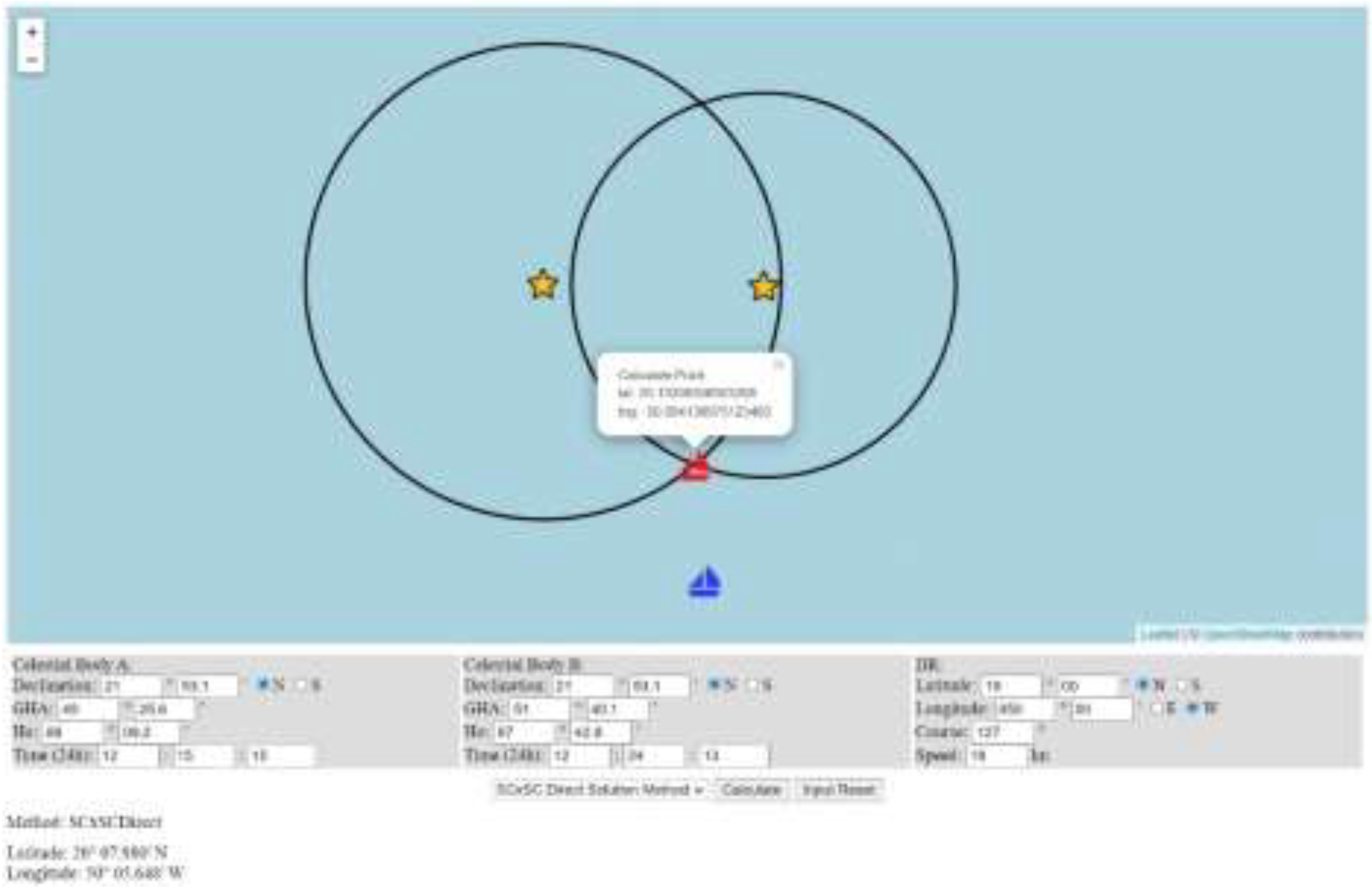
5.2. Sun-Run-Sun Observation Fix

Example 2. On 31 May 1975, ZT 12-24-00, a vessel’s dead reckoning position, was 19°00.0′ N latitude and 050°00.0′ W longitude. The ship was on course at 127° and a speed of 18 knots. The navigator observed the lower limb of the sun twice. The observation data determined the celestial positioning at ZT 12-24-13, as shown in

Table 4. The observations data for solving the celestial positioning in Example 2.

Celestial Body	Sun	Sun
Zone Time	12-15-15	12-24-13
Declination	21°53.1′ N	21°53.1′ N
GHA	49°25.6′	051°40.1′
Ho	88°09.2′	87°42.8′

, which has been rewritten from [1].

Example 2 shows that the method that is proposed in this paper is accurate and can be widely used in celestial positioning. The celestial positioning (latitude 20°07.980′ N and longitude 050°05.648′ W) was determined using Newton’s method and the closed analytical solution method. The results are shown in Figure 9 and Figure 10 and Table 5.

Table 5. The results of Example 2 of sun-run-sun observation fix.

Method	Latitude	Longitude
Sumner-GC Approach	20°08.0′ N	50°05.7′ W
Sumner-SL Approach (Chen et al., 2015) [10]	20°08.0′ N	50°05.7′ W
MSM (Hsu et al., 2017) [11]	20°08.0′ N	50°05.7′ W
Scenario 1 Newton’s Method	20°07.980′ N	50°05.648′ W
Scenario 2 Closed Analytical Solution Method	20°07.980′ N	50°05.648′ W

Table 5. The results of Example 2 of sun-run-sun observation fix.

Method	Latitude	Longitude
Sumner-GC Approach	20°08.0′ N	50°05.7′ W
Sumner-SL Approach (Chen et al., 2015) [10]	20°08.0′ N	50°05.7′ W
MSM (Hsu et al., 2017) [11]	20°08.0′ N	50°05.7′ W
Scenario 1 Newton’s Method	20°07.980′ N	50°05.648′ W
Scenario 2 Closed Analytical Solution Method	20°07.980′ N	50°05.648′ W

Figure 9. The GUI of Newton’s method calculation program (for Example 2).

Figure 9. The GUI of Newton’s method calculation program (for Example 2).

Figure 10. The GUI of the closed analytical solution method calculation program (for Example 2).

Figure 10. The GUI of the closed analytical solution method calculation program (for Example 2).

Furthermore, our algorithm can improve the positioning accuracy and satisfy the requirements of celestial navigation. Compared with the results of other theses, our results are not limited by the scale of the nautical chart.

5.3. Comparison with Celestial Positioning of Other Closed Analytical Solution Methods

Example 3. On 1 September 1975, GMT 00-00-00, a vessel’s dead reckoning position was at 41°39.7′ N latitude and 091°31.9′ W longitude. At the same time, the navigator observed the Arcturus, Altair, Antares, and Vega. The observation data determined the celestial positioning at GMT 00-00-00, as shown in

Table 6. The observation data for solving the celestial positioning in Example 3.

Celestial Body	Arcturus	Altair	Antares	Vega
Greenwich Mean Time	00-00-00	00-00-00	00-00-00	00-00-00
Declination	19°19.02′ N	8°47.94′ N	26°22.56′ S	38°45.54′ N
GHA	125°54.9′	042°09.36′	092°34.86′	60°31.2′
Zenith Distance	36°42.24′	54°22.92′	68°02.7′	23°43.86′
Ho	53°17.76′	35°37.08′	21°57.3′	66°16.14′

, which has been rewritten from [4].

The results were verified according to the heuristic article [4] of this study’s celestial positioning method, as shown in

Table 7. The results of Example 3.

	James A. Van Allen Method		Scenario 2 Closed Analytical Solution Method
Celestial Bodies	Position 1	Position 2	Position 1	Position 2
Arcturus–Altair	41°39.66′ N 091°31.92′ W	2°08.88′ S 095°36.3′ W	41°39.690′ N 091°31.925′ W	2°08.904′ S 095°36.311′ W
Arcturus–Antares	41°39.72′ N 091°31.92′ W	0°08.16′ N 157°50.46′ W	41°39.725′ N 091°31.949′ W	0°08.164′ N 157°50.460′W
Arcturus–Vega	41°39.66′ N 091°31.92′ W	29°20.04′ N 086°57.0′ W	41°39.677′ N 091°31.916′ W	29°20.038′ N 086°57.024′ W
Vega–Antares	41°39.72′ N 091°31.92′ W	21°00.54′ N 042°11.16′ W	41°39.724′ N 091°31.920′ W	21°00.564′ N 042°11.136′ W
Vega–Altair	41°39.72′ N 091°31.92′ W	62°17.7′ N 055°33.0′ W	41°39.701′ N 091°31.918′ W	62°17.713′ N 055°33.021′ W
Altair–Antares	41°39.72′ N 091°31.92′ W	37°08.58′ S 011°05.22′ W	41°39.724′ N 091°31.906′ W	37°08.589′ S 011°05.214′ W

.

The results of the celestial positioning from these two closed analytical solution methods were compared in terms of the yielded latitude and longitude measurements. The differences between the two sets of numbers were very small, as shown in

Table 8. Latitude errors of the two positioning methods.

		James A. Van Allen Method	Scenario 2 Closed Analytical Solution Method
Celestial Bodies		Latitude	Latitude	Error
Arcturus–Altair	Position 1 Position 2	41°39.66′ N 2°08.88′S	41°39.690′ N 2°08.904′ S	−0.00049154 0.00039597
Arcturus–Antares	Position 1 Position 2	41°39.72′ N 0°08.16′ N	41°39.725′ N 0°08.164′ N	−7.65824 × 10−5 −6.71714 × 10−5
Arcturus–Vega	Position 1 Position 2	41°39.66′ N 29°20.04′ N	41°39.677′ N 29°20.038′ N	−0.000277142 3.96043 × 10−5
Vega–Antares	Position 1 Position 2	41°39.72′ N 21°00.54′ N	41°39.724′ N 21°00.564′	−7.02238 × 10−5 −0.00040464
Vega–Altair	Position 1 Position 2	41°39.72′ N 62°17.7′ N	41°39.701′ N 62°17.713′ N	0.000306181 −0.00021584
Altair–Antares	Position 1 Position 2	41°39.72′ N 37°08.58′S	41°39.724′ N 37°08.589′ S	−6.70762 × 10−5 0.000147566

and

Table 9. Longitude errors of the two positioning methods.

		James A. Van Allen Method	Scenario 2 Closed Analytical Solution Method
Celestial Bodies		Longitude	Longitude	Error
Arcturus–Altair	Position 1 Position 2	091°31.92′ W 095°36.3′ W	091°31.925′ W 095°36.311′ W	8.228 × 10−5 0.00019469
Arcturus–Antares	Position 1 Position 2	091°31.92′ W 157°50.46′ W	091°31.949′ W 157°50.460′ W	0.000479874 1.59876 × 10−06
Arcturus–Vega	Position 1 Position 2	091°31.92′ W 086°57.0′ W	091°31.916′ W 086°57.024′ W	−6.34249 × 10−5 0.000394446
Vega–Antares	Position 1 Position 2	091°31.92′ W 042°11.16′ W	091°31.920′ W 042°11.136′ W	−1.45425 × 10−06 −0.000407289
Vega–Altair	Position 1 Position 2	091°31.92′ W 055°33.0′ W	091°31.918′ W 055°33.021′ W	−3.08622 × 10−5 0.000360546
Altair–Antares	Position 1 Position 2	091°31.92′ W 011°05.22′ W	091°31.906′ W 011°05.214′ W	−0.000239639 −9.69143 × 10−5

. Hence, they could be considered to have the same celestial positioning. However, the method that is proposed in this paper is simpler and more visual, hence it is suitable for university-level students to learn.

6. Discussions

The time that was required for the computer execution process of the two methods that are proposed in this paper (Scenario 1 and Scenario 2) was very short, with the time for Scenario 1 being 40~50 μs and Scenario 2 being 20~30 μs. The execution time of Scenario 2 was about 10 μs shorter and this method’s consumption of computer execution resources was lower. Nevertheless, the execution time of the two methods is below the unit of seconds, meaning that their calculation speed is rapid.

If Scenario 1 was used for calculation, the iterative operation was required. Notably, the number of iterations usually exceeded 3 or more, so the convergence speed was slow. Only a celestial fix that was close to the reference position could be obtained. Meanwhile, the position of another intersection could not be calculated. Scenario 2 was free of iterative operation, had a faster calculation process, and had better stability than Scenario 1 and the methods that have been proposed in other studies. However, when Scenario 2 was used in other areas (e.g., location-based services [LBS]), the small circle computation number increased, e.g. C(100, 2). In this example, there would be 4950 combinations without repetition and Scenario 2 would be more advantageous in this case. Certainly, both methods have a graphical user interface (GUI), which is the optimal tool for celestial navigation teaching. The aforesaid methods can also be considered as alternative schemes for GNSS.

7. Conclusions

This study presented a new improvement in celestial navigation, in which coordinate transformation and vector algebra are applied instead of using the spherical trigonometry method. The derivation of the equation is straightforward and intuitive. Because the proposed algorithm has a reference position (DR, EP, and AP), the correct ship position can be selected regardless of the use of Scenario 1 or Scenario 2 and misjudgment can be avoided. Compared with methods that have been presented by other studies, Scenario 2 is more straightforward and the celestial positioning can be obtained without iteration. Additionally, it can be integrated with an ECDIS and stand as an ancillary GNSS option. The algorithm that is used in this paper is suitable for the syntax of computer algorithms and commercial mathematics software. Furthermore, it contributes to some improvements in the celestial navigation method, making the method more modern and accurate. Moreover, this algorithm can explain the celestial navigation principles more clearly to maritime school students.

References

- Bowditch, N. American Practical Navigator; Defense Mapping Agency Hydrographic Center: Bethesda, MD, USA, 1995. [Google Scholar]
- Cutler, T.J. Dutton’s Nautical Navigation; United States Naval Institute: Annapolis, MD, USA, 2004. [Google Scholar]
- Navy, R. The admiralty manual of navigation. In The Principles of Navigation; United States Naval Institute: Annapolis, MD, USA, 2008. [Google Scholar]
- Van Allen, J.A. An analytical solution of the two star sight problem of celestial navigation. J. Navig. 1981, 28, 40–43. [Google Scholar] [CrossRef]
- Chen, C.-L.; Hsu, T.-P.; Chang, J.-R. A novel approach to determine the astronomical vessel position. J. Mar. Sci. Technol. 2003, 11, 221–235. [Google Scholar] [CrossRef]
- Gonzalez, A.R. Vector solution for the intersection of two circles of equal altitude. J. Navig. 2008, 61, 355–365. [Google Scholar] [CrossRef]
- Pierros, F. Stand-alone celestial navigation positioning method. J. Navig. 2018, 71, 1344–1362. [Google Scholar] [CrossRef]
- Tsou, M.-C. Genetic algorithm for solving celestial navigation fix problems. Pol. Marit. Res. 2012, 19, 53–59. [Google Scholar] [CrossRef] [Green Version]
- Tsou, M.-C. Celestial navigation fix based on particle swarm optimization. Pol. Marit. Res. 2015, 22, 20–27. [Google Scholar] [CrossRef] [Green Version]
- Chen, C.-L.; Hsu, T.-P.; Weng, G.-Y. New computational approaches to determining the astronomical vessel position based on the Sumner line. Pol. Marit. Res. 2014, 21, 3–11. [Google Scholar] [CrossRef] [Green Version]
- Hsu, T.-P.; Weng, G.-Y.; Chen, C.-L. A modified Sumner method for obtaining the astronomical vessel position. J. Mar. Sci. Technol. 2017, 25, 319–328. [Google Scholar]
- Yabuki, H. The 2010 Manila amendments to the STCW convention and code and changes in maritime education and training. J. Marit. Res. 2011, 1, 11–17. [Google Scholar]
- Capolupo, A.; Monterisi, C.; Saponieri, A.; Addona, F.; Damiani, L.; Archetti, R.; Tarantino, E. An interactive Web GIS framework for coastal erosion risk management. J. Mar. Sci. Eng. 2021, 9, 567. [Google Scholar] [CrossRef]
- Earle, M.A. Vector solutions for great circle navigation. J. Navig. 2005, 58, 451–457. [Google Scholar] [CrossRef]
- Tseng, W.-K.; Lee, H.-S. Building the latitude equation of the mid-longitude. J. Navig. 2007, 60, 164–170. [Google Scholar] [CrossRef]
- Tseng, W.-K.; Lee, H.-S. The vector function for distance traveled in great circle navigation. J. Navig. 2007, 60, 158–164. [Google Scholar] [CrossRef]
- Dutton, B.; Maloney, E.S. Dutton’s Navigation & Piloting; United States Naval Institute: Annapolis, MD, USA, 1985. [Google Scholar]