Article

Hierarchical Optimization of Oil Spill Response Vessels in Cases of Accidental Pollution of Bays and Coves

by
Marko Đorđević
1,
Đani Mohović
1,*,
Antoni Krišković
1 and
Tarzan Legović
2,3,4
1
Faculty of Maritime Studies, University of Rijeka, Studentska 2, 51000 Rijeka, Croatia
2
Faculty of International Relations and Diplomacy, Libertas International University, Trg J.F. Kennedy 6b, 10000 Zagreb, Croatia
3
Laboratory for Data Science, Oikon, Trg Senjskih Uskoka 1-2, 10020 Zagreb, Croatia
4
Division for Marine and Environmental Research, R. Bošković Institute, Bijenicka Cesta 54, 10000 Zagreb, Croatia
*
Author to whom correspondence should be addressed.
J. Mar. Sci. Eng. 2022, 10(6), 772; https://doi.org/10.3390/jmse10060772
Submission received: 27 April 2022 / Revised: 27 May 2022 / Accepted: 30 May 2022 / Published: 2 June 2022
(This article belongs to the Section Marine Pollution)

Abstract

:
Ships pollute bays and coves with oils daily. Although the number of major pollution events is decreasing, accidents still occur and are likely to occur in the future. Most often, pollution arises from spills of non-persistent oil in bays, mainly during the summer season. A prompt response is key to oil collection success in semi-enclosed waters. In order to ensure that oil does not reach the mainland and endanger a potentially crucial economic resource of a country, it is vital to collect it in minimal time. Furthermore, it is also essential to send response ships that minimize the cost. In practice, there may be several optimal combinations of response ships to be sent. When the response cost is considered, obtaining all possible optimal solutions (a complete Pareto front) is vital because the shortest collection time does not necessarily mean the lowest costs. For these reasons, two general optimization models are considered. The first model gives the minimum response time to collect oil from the sea’s surface, while the second model gives the minimum response cost of ships participating in the clean-up operation. The supplied pseudo-codes allow for all optimal solutions to be found.

1. Introduction

Today, transporting goods and cargo by sea is the most economical transport branch [1]. Some types of cargo require special attention during transport and handling while loading and unloading in ports. World sea transport involves cargo with different properties [2]. Historically, liquid cargo tankers have influenced marine ecology significantly [3,4]. Preventing the spread of oil on the sea surface during transport is crucial [5]. Knowledge of the characteristics of the spilled oil is an essential factor in the application of appropriate intervention measures, including operational staff [6]. In addition, the allocation of maritime oil spill combat ships is crucial [7]. It should be emphasized that each maritime accident and each oil spill should be considered separately [8,9] (p. 1). The frequency of oil pollution will be significantly reduced by applying preventive measures, but oil spills are possible anywhere and anytime despite prevention [10,11,12]. For these reasons, an efficient system is needed to respond to accidental marine pollution in order to maximally reduce the damage.
In a thorough review, Weiwei et al. (2015) [13] claimed that in the event of a large oil spill at sea, often more than one oil spill emergency vessel should be dispatched. Furthermore, they analysed the state-of-the-art characteristics of emergency disposal programs for marine oil spills and the requirements for emergency vessel scheduling. Their research demonstrated that integrating multiple technologies, such as ad-hoc networks, GPS, and AIS, can improve the operational capacity of emergency vessels on-site and minimize damage caused by offshore oil spills. The research gap is that the study showed the schedule of the response ships but did not give an answer as to which combination of response ships to send toward oil slicks. Li et al. (2019) [14] provided a systematic literature review of the methodology for emergency materials to be dispatched based on three main steps combined with the development of China’s oil spill response capacity. The first step is to intervene in large marine spills. Second, following different grade accidents, the demand for all available emergency materials is replaced by an equivalent total volume. The third step lists the conditions for the emergency materials to be dispatched to minimize the arrival times of all oil spill emergency disposal vessels. The shortcoming of the study was that the authors calculated the fastest arrival of ships to the place of the spill, but this does not necessarily mean that the fastest remedial action will happen because the rate of collecting oil from the sea surface was not considered.
Ye et al. (2019) [15] focused on how to improve marine oil spill response efficiency to minimize environmental and socioeconomic impacts. They proposed a new simulation-based multi-agent particle swarm optimization (SA-PSO) approach for supporting marine spill decision-making through the integrated simulation and optimization of response device allocation and process control. The authors did not consider different types of oils. Each type of oil affects flora and fauna differently and requires different types of skimmer devices. Ye et al. (2021) [16] suggested an emergency response system based on dynamic process simulation and system optimization modelling. Furthermore, the authors suggested a particle swarm optimization (ME-PSO) algorithm with outstanding convergence performance and low computational cost characteristics that integrated multi-agent theory and evolutionary population dynamics. Most authors have used linear programming, multi-criteria analysis, or genetic algorithms. A genetic algorithm was also used to allocate specialized vessels. The model proposed in this paper concerning the mentioned models takes the capacity of an individual skimmer device to be a more accurate measure in the calculation of the spill response time. Furthermore, it is important to emphasize that the pollution of bays and coves is more frequent than large accidents at sea [17]. As previously pointed out, oil spills should be considered separately precisely because there are different types of oils, behaviours, and movements on the sea surface. For these reasons, the basic properties of oil were reviewed from an analytical and graphical point of view. Using the ADIOS program, the properties of Arabian extra light (Aramco) oil can be viewed graphically in real time.
The two general models proposed in this paper can be applied to any bay or cove in the world. The first model gives the minimum number of response ships that have a tank capacity sufficient enough to collect the oil slick, taking into account that the duration of collecting pollution from the sea will be the shortest. The second proposed model considers the cost of the response ship per hour of operation. Thus, in the case of pollution, the commander in charge of the response to accidental marine pollution can choose a response, taking into account the minimum duration of collecting pollution from the sea or using the model and strategy to reduce costs. The presentation of the results from the two models is given using the example of the Rijeka Bay area. It is important to emphasize that proper handling of personal protection and specialized equipment and following the intervention plan must not be neglected in order to reduce the risk of pollution and take the optimal action. The two general models proposed here enable selecting the optimal number of response ships sent to collect oil spills in bays or coves. The contribution of the article includes several possible optimal solutions with the selection of the optimal time of response to pollution or reducing remediation costs. The proposed models can thus significantly help ports and bays respond to accidental oil pollution.
The paper is organized as follows: First, oil behaviour in marine environments is reviewed, and then methods of finding optimum sets of ship combinations to collect oil are elaborated. Pseudo-codes of the presented methods can be found in the appendices. The results and verification of the models are presented next using several examples, including the data from Rijeka Bay. In the discussion, various application issues are mentioned. The conclusion emphasizes the value of the obtained results in combating oil pollution in bays and semi-enclosed seas.

2. Maritime Spill Accidents and Oils Behaviour in the Marine Environment

Advances in technology have enabled maritime transport to develop faster, but freight prices have risen significantly due to the recent coronavirus pandemic [18] and war. Throughout history, liquid cargo ships have significantly influenced marine ecosystems [19]. However, other types of vessels that can dramatically pollute the sea and coast should not be neglected. For example, container vessels are also increasing to reduce transport costs, but they have larger fuel tanks, which, in the case of an accidental oil spill, can cause significant damage to flora and fauna [19,20]. The main goal of cleaning up accidental pollution is to collect the spilled oil from the sea surface as quickly as possible before it dissolves in the seawater or reaches the coast or other economically significant resources of a particular country and protect human lives [21]. Figure 1 shows two categories of marine pollution with oil. The amounts of pollution shown were caused by liquid cargo ships. The first category is in the domain of over 700 tons of oil spilled on the sea surface and is shown in the colour green. The blue colour shows pollution in the range of 7–700 tons. It should be emphasized that 7–700 tons of oil is much more common than large oil spills of over 700 tons. Furthermore, the red line shows the average marine pollution per year.
It is essential to emphasize the characteristics of oils. The physical and biological effects of an oil spill, the behaviour of the oil slick, and the effectiveness of different cleaning methods largely depend on the type of oil spilled [23]. Furthermore, the physical and chemical characteristics determine the thickness of the layer of oil, the rate of spread of the oil slick, and consequently, the selection of the most suitable cleaning technique [24]. The physical and chemical characteristics of oil that determine its behaviour on water and the effectiveness of cleaning operations include its density, viscosity, evaporation, dispersion, and changes in these parameters over time [25]. The physical properties of the oil will vary depending on local conditions and may deviate significantly from the values that exist in the standards. Most often, pollution arises from a spill of non-persistent oil in bays, mainly during the summer season [26]. So, we decided to analyse weathering processes using ADIOS (NOAA’s oil weathering model) for oil types, using Arabian extra light (Aramco) as an example.
Figure 2 shows changes in oil density over time. Oil density affects the rate of oil dispersion in water. The American Petroleum Institute (API) scale (density), which is based on pure water, is often used, which determines the API value of 10% mass by agreement [27].
Figure 3 shows changes in oil viscosity over time. Viscosity is a measure of the internal resistance of a fluid. The lower the viscosity of a substance, the easier it flows [28]. Honey is usually an example of a high viscosity liquid. Temperature affects viscosity as well as other physical characteristics of oil [28,29]. The lower the temperature, the higher the viscosity. The viscosity is determined by the amount of lighter fractions that the oil contains and the ambient temperature [30]. Regarding the cleaning of the oil spill, the viscosity affects the spread of the slick, the stickiness of the oil, its penetration into the soil and sediments of nearby beaches, and the possibility of pumping the oil from the surface [31].
Figure 4 shows an example of oil budget and weathering, including the evaporation and dispersion of spilled oil. It is essential to point out that volatile fractions are lost to the atmosphere, and the rate of evaporation is determined by the type of oil, wind speed, and ambient temperature [32]. A wavy sea promotes evaporation, and the rest of the oil that does not evaporate has a higher density and is more viscous [33]. It can also be seen in the graph how evaporation causes a loss of oil mass at sea. Most crude oils lose up to about 40% of their volume in a few hours [34], while products such as gasoline and light diesel evaporate completely in a few hours [35]. Figure 4 also shows the rate of oil dispersion after contact with the sea surface. It should be emphasized that the waves tear the surface covered by oil into smaller patches and thus improve the dispersion of the oil [36]. Smaller droplets remain in the water column, while larger droplets rise again to the sea surface. The dispersion rate depends on the type of oil spilled and the state of the sea [37]. The spread and decomposition of oil are directly affected by the state of the sea with parameters such as the wind, sea currents, sea depth, and waves. The wind is a factor that affects the behavior and conditions of the oil. Wind and sea conditions have the most significant effect on the speed of oil movement, which reaches 2.5 to 4% of the wind speed [38].

3. Materials and Methods

Several optimization strategies are suggested. In all strategies, two-level hierarchical optimization is used. The allocation scenario is a combination in which each response ship is associated with an appropriate amount of oil to collect. For each response ship in the scenario, this quantity is less than or equal to the maximum capacity of the response ship (known value prior to the accident) and strictly greater than zero. Additionally, it is assumed that all response ships, except one at most, will have an allocated amount equal to their maximum capacity. In all of the strategies, it is assumed that each response ship will participate in the operation once at most and that there is at least one scenario of available response ships whose total capacity is greater than or equal to the volume of pollution. We started each strategy with a set of all possible scenarios without allocation. In the first stage of all strategies, scenarios whose total capacity is strictly less than the amount of pollution are rejected. Taking into account the previous assumption, this means that there exists at least one strategy that will not be rejected in this step. The flowchart for Stage 1 is given in Figure 5.
The rest of the algorithm is different for each strategy, and the details are given below.
Strategy 1
The first strategy uses optimization at the following two levels:
  • The minimum number of response ships involved in the operation,
  • The shortest operation duration (includes collection only).
This strategy does not take into account the time of arrival of the response ships but only the time of collection. In other words, it is assumed that all response ships are equidistant from the place of pollution (for example, a fleet stationed in one port) and that they have the same sailing speed. Note that the cost of the operation is not taken into account in this strategy. In this strategy, the input values of the algorithm are as follows:
  • The amount (volume) of pollution;
  • Data on available response ships, i.e., for each ship. the following is known:
    • Maximum capacity (m3);
    • Collection rate (m3/h).
In the second stage of this strategy, the optimization procedure with regard to the number of response ships in the scenario (first level of optimization) is carried out by determining for each scenario the number of ships involved in that scenario, and then the minimum number of ships in all scenarios. All scenarios that include more than the minimum number of response ships needed to collect the oil are rejected. In the third stage for each of the remaining scenarios, the allocation of the amount of pollution for all ships in the scenario is carried out. Note that due to the second stage in each remaining scenario, all ships must be allocated some of the total amount of pollution (otherwise, there is a contradiction with the minimum selection at the first level). In addition, due to the assumption that all but one ship at most must have an allocated maximum capacity, the allocation is carried out as follows: For each scenario, the maximum collection time for each ship is calculated. The full capacity is then allocated to all vessels except the one with the longest maximum collection time. The vessel with the longest maximum collection time is allocated the remaining amount of pollution (total amount of pollution reduced by the total capacity of other ships in this scenario). After this stage, the allocation scenario is known. In the last (fourth) stage, minimization is performed with respect to the duration of the collection operation (second level of optimization). For each allocation scenario, an operation duration (equal to the maximum collection time for response ships in that scenario) is determined, and then a minimum operation duration is determined among all scenarios. All the scenarios that have a duration of operation longer than the minimum are rejected. The scenarios remaining after the fourth stage are optimal with regard to Strategy 1. The pseudo-code corresponding to the algorithm described above is given in Appendix A.
Strategy 2
In the second strategy, the additional input of parameters is taken into account. As in the first strategy, for each available response ship, the following is known:
  • Ship capacity (m3);
  • Collection rate (m3/h).
In addition, in this strategy, equidistance is no longer assumed. Furthermore, ships may differ in their speed of sailing and in the cost of participating per unit of time, so the following is also known for each ship:
3.
Distance from the oil slick (km);
4.
Average sailing speed (km/h);
5.
Price of participation in the operation (EUR/h).
In Strategy 2, the following two optimization criteria are used:
  • Minimum total duration of the operation (includes the start and duration of collection);
  • Minimum cost of participating in the operation (includes travel and collection).
In the two versions of this strategy, there are different hierarchical arrangements of the two listed optimization criteria, as shown in Table 1.
After the application of the first stage, which is the same for all strategies and in which all scenarios with insufficient total capacity have been removed, there may be many combinations left, i.e., scenarios in which not all response ships are allocated some capacity, while maintaining the assumption that all ships in the scenario have a capacity allocation greater than zero, and all but a maximum of one have their maximum capacity allocated. In order to reduce the computational complexity of the algorithm in the process of implementing the optimization criteria, in the second stage, first, all of the suboptimal scenarios are discarded. An easy way to do this is for all scenarios that still have the total capacity to collect pollution when a ship with the lowest capacity is rejected from them to be declared suboptimal. The flowchart for Stage 2 of Strategies 2a and 2b is given in Figure 6.
The remaining stages in the two versions differ, and the general idea is as follows. In the third stage, for each combination, the corresponding allocation scenario is determined so that all response ships except the one with the maximum target value with respect to the first optimization criterion (maximum duration in Strategy 2a and maximum cost in Strategy 2b) are allocated their full capacity. The remaining ship is allocated a capacity equal to the remaining amount of pollution. Then, for each scenario, the value of the objective function given by the first optimization criterion is calculated (duration of the operation in Strategy 2a and total cost in Strategy 2b) and the corresponding minimum value of the objective function across all remaining scenarios. At the end of this stage, all scenarios that have a value of the objective function strictly greater than the minimum are rejected. In the last, fourth phase, for each remaining allocation scenario, the corresponding value of the objective function is calculated according to the second optimization criterion (total cost in Strategy 2a and duration of the operation in Strategy 2b), and then the minimum value among them is selected. Finally, all scenarios that have a value of the objective function strictly higher than the determined minimum are rejected. General flowchart for all strategies is given in Figure 7. Figure 8 shows flowchart for stage 2 of strategy 1.

4. Verification of Models and Results

In this section, several examples are used to test and verify the algorithms described in the previous section on several examples. In Example 1, Strategy 1 is tested. The input data related to the response ship characteristics are given in Table 2. Let the volume of pollution be P = 10 m3. In practice, the volume will have the greatest uncertainty. Hence, one should use a higher rather than a lower estimate.
The results below are given for each intermediate step in the algorithm i.e., the output after each phase and the final result. The output of Stage 1 is given in Table 3, in which 1 indicates that the corresponding ship is participating in the given scenario and 0 indicates that it is not participating. Scenarios differ by the ships involved. There are 10 scenarios in which the total capacity of the response ships involved is sufficient to collect the oil spill, i.e., greater than or equal to the value of P = 10 m3. The table shows that the minimum number of ships included in the scenario is two. After Stage 2, the scenarios listed in Table 4, i.e., those scenarios from Table 3 that include exactly two response ships. Stage 3 allocates the amount of pollution for the scenarios in Table 4 according to the criterion of the minimum duration of the operation, as described in the previous section. The results of the allocation (in m3) are recorded in Table 5. Table 6 presents the durations (h) of operation for individual ships. The scenarios have the durations of 16 h, 13 h, 13 h, 15 h, and 15 h, respectively, and the minimum duration is 13h.
Therefore, after Stage 4, the final output of the algorithm is calculated, that is, Scenarios 2 and 3. This is also the final output of Strategy 1, which means that, in Example 1, there are two global minima. In Example 2, the input data related to the ship characteristics of Strategies 2a and 2b are given in Table 7. Let the volume of pollution be P = 25 m3.
A list of possible scenarios after Stage 1 is given in Table 8. This list also includes scenarios that contain too many response ships, i.e., the scenarios that do not allow allocation in accordance with the description of the strategies. For example, in Scenario 10, it is not possible to meet the principle that one ship at most does not collect its full capacity. The results after Stage 2, in which the surplus ship scenarios are rejected, are presented in Table 9. The first two stages, as well as the corresponding results, are the same for both Strategies 2a and 2b. In Strategy 2a, Stage 3 is optimized in terms of duration, and Stage 4 in terms of cost. The results after Stage 3 are presented in Table 10, Table 11 and Table 12. It can be seen that the minimum duration is 14h, and the total cost of both scenarios is equal to 43 EUR. Therefore, the results after Stage 4 are the same as after Stage 3, and they are equal to the final output of the algorithm. So, there are two optimal scenarios under Strategy 2a. The flowchart for stage 3 of strategy 1 is given in Figure 9. Figure 10 shows flowchart for stage 4 of strategy 1. In Example 2, for final allocation, duration and cost for strategy 2a is given in Table 10, Table 11 and Table 12.
In Strategy 2b, Stage 3 is optimized in terms of cost and Stage 4 in terms of duration. The results after Stage 3 are presented in Table 13, Table 14 and Table 15. The minimum cost is 29 EUR, and the scenarios have a duration of 17 h, 16 h, and 16 h, respectively. Thus, after Stage 4, two scenarios remain, Scenarios 5 and 6, which are also the two final solutions to the problem under Strategy 2b. Clearly, the optimal solutions found by Strategies 2a and 2b differ. The flowchart for stage 3 of strategy 2a is given in Figure 11. Figure 12 shows flowchart for stage 4 of strategy 2a. In Example 2, for final allocation, duration and cost for strategy 2b is given in Table 13, Table 14 and Table 15.
Example 3
In this example, all strategies were tested on realistic input data for Rijeka Bay. Input data related to the response ship characteristics are given in Table 16. The hypothetical amount of pollution was P = 10 m3 and the price was 500 EUR/h.
According to Strategy 1, we obtained two optimal scenarios. In the first scenario, only the ship EKO 2000 participates with its maximum capacity, and the duration of the operation is 1.67 h. In the second optimal scenario, only the ship EKO 12,000 with its full capacity participates, and the operation lasts 1.67 h. Strategies 2a and 2b give the same results. This is the optimal scenario in which only the ship EKO 2000 participates with its maximum capacity. The total duration of the operation is 2.21 h, and the cost is 1373.29 EUR. Additionally, the model results may be significantly affected only by the uncertainty of the volume of oil spilled. The rest of the parameters are subject to small errors. The flowchart for stage 3 of strategy 2b is given in Figure 13. Figure 14 shows flowchart for stage 4 of strategy 2b.

5. Discussion

In response to the accidental pollution of bays and coves, the following variables are taken into account: the number of existing response ships, the variable rate of oil collection (skimmers) installed on each ship, the capacity (volume) of tanks on a response ship, the sailing speed of an individual response ship, the distance of an individual response ship to the place of pollution, and the cost of the response ship taken in the model to be calculated per hour of ship operation. The number of existing ships may vary depending on the pollution area or the country responsible for the area. There are different types of skimmer devices on ships. Each skimmer has a different oil collection rate; in addition, skimmers can differ in selectivity so that one skimmer can collect more seawater than another [39]. All this can affect the accuracy of the model. Furthermore, there are different skimmer devices such as disk skimmers and brush skimmers. In practice, the disk skimmer is used for non-persistent oils that are much more common in bays and coves, but we must not ignore the fact that there is pollution with bunker fuel even in closed areas [40]. Bunker fuel is a persistent oil and, as such, requires removal with a brush skimmer. The rates of disk and brush skimmers are different. The choice depends on the person handling the ship and the collection rate of the skimmer [41]. The rate of oil collection from the sea surface also varies. In addition, the response ship may have more than one skimmer device installed. Furthermore, when looking at the pollution collection capacity, one ship can vary from 30 m3 to 45 m3. Ship speeds are also variable, and the distance of ships to the oil slick often varies [42]. The above indicates that the model must be general. The developed pseudo-codes represent two models where one can insert the values of variables prior to and with the first known information of the accident. The models may be used for any bay or cove in the world. Verification of the models was performed on several theoretical examples, and finally, the models were tested with accurate data for the Rijeka Bay area. As pointed out, in the given problem of minimizing the time required to remove pollution from the sea, there are several optimal solutions. Using software tools such as Matlab, Python, and R programs can provide only one optimal solution. The programs show, for example, the first and fourth ships as the optimal solution for the minimum time of oil removal, while the combination of the first and third ships also gives the same collection time. Not considering all possible solutions can lead to a suboptimal result when multiple variables are considered. For these reasons, it was necessary to program such models and construct pseudo-codes that will allow for finding all optimal solutions [43]. Furthermore, there is a contradiction when optimizing for the duration of removing oil from the sea surface or optimizing for the costs. For example, if there are two ships, and one ship collects oil for 3 h, and the other ship collects for 5 h, the total collection time is 5 h. However, when the cost of the ship per hour is taken into account, it is necessary to pay for eight working hours. In the second example, two ships collect oil for 4.5 h, and the total time is 4.5 h, which leads to the conclusion that this is a more optimal solution when looking at the duration of the cleaning action. However, the cost of these two ships is more expensive than the first two ships. For this reason, two models and two types of optimization strategies are proposed. The command team is thus given the option to choose between the optimal number of ships to keep collection time to a minimum (for example, when the oil slick is close to a coast) or to optimize the cost (when the oil slick is far from the coast).

6. Conclusions

Rapid response to accidental pollution in bays is the key to combating oil slicks on the sea surface close to the coast. The two proposed models help in choosing the optimal number of response ships, aiming to shorten the response time to accidental pollution or to minimize the cost. The proposed first model selects the minimum number of ships sufficient to remove pollution from the sea, considering the shortest response time. The oil will be removed from the sea surface as quickly as possible, preventing further pollution and preserving critical economic areas. The model also contributes to the protection of nearby beaches, nature parks, or other country resources. It is essential to know exactly how many ships and which ships meet the criteria for collecting a specific volume of spilled oil while keeping costs to a minimum. The proposed second model provides the optimal number of ships that meet the criteria for collecting oil slicks from the sea while minimizing the response costs. Furthermore, it is essential to point out that knowing the characteristics of the spilled oil and its properties, such as its viscosity and evaporation, helps in choosing specialized equipment to respond to marine pollution. The proposed models may contribute to the development of intervention plans, and preventive measures, and ultimately raises the likelihood of marine environment protection following an oil spill.

Author Contributions

Conceptualization, M.Đ. and T.L.; Methodology, Đ.M. and T.L.; Software, M.Đ. and A.K.; Validation, M.Đ., Đ.M., T.L. and A.K.; Formal Analysis, Đ.M.; Investigation, M.Đ.; Resources, T.L.; Data Curation, M.Đ.; Writing—Original Draft Preparation, M.Đ. and Đ.M.; Writing—Review and Editing, M.Đ. and T.L.; Visualization, A.K. and T.L.; Supervision, M.Đ. and Đ.M.; Project Administration, Đ.M. All authors have read and agreed to the published version of the manuscript.

Funding

This research received no external funding.

Institutional Review Board Statement

Not applicable.

Informed Consent Statement

Not applicable.

Data Availability Statement

The statistical data of accidents close to the Croatian Coast of the Adriatic Sea are available at the official archive of the “Republic of Croatia—Ministry of the Sea, Transport and Infrastructure” at the following link: https://mmpi.gov.hr/more-86/traganje-i-spasavanje-109/statistika/13773. The statistical data on fishing can be found at the official website of the Croatian Ministry of Agriculture: https://ribarstvo.mps.hr/default.aspx?id=45. The statistical data on tourism can be found at the official archive of the “Republic of Croatia—Ministry of Tourism and Sport”: https://mint.gov.hr/pristup-informacijama/dokumenti-80/statistike/arhiva-12059/12059 (accessed on 1 June 2022).

Conflicts of Interest

The authors declare no conflict of interest.

Appendix A. Pseudocodes

Algorithm A1: Strategy 1
Input: Matrix of response ships data A (A has n rows, where n is number of available ships; the columns are as follows: A[:, 1] (the first column of A)—ship capacity in m3; A[:, 2] (the second column of A)—oil collection rate in m3/h); volume of pollution: P in m3.
Output: Number of optimal scenarios k; matrix of optimal scenarios M (M has k rows and n columns; M[i,j]—quantity of pollution assigned to ship j in solution i), matrix of duration for each scenario: T (T has k rows and n columns, T[i,j]—duration of operation of ship j in scenario i); duration of operation T_min.
1Initialization: M is the matrix of all possible solutions (M has binary entries, 2n−1 rows and n columns, M[i, j] = 0 means that ship j is not assigned and M[i, j] = 1 means that ship j is assigned in the i-th solution.); k = 2n−1.
Stage 1: Elimination of scenarios with insufficient capacity
2for i = 1, 2,…, k do:
3      if the dot product of M[i, :] and A[:, 1] (the total capacity of ships in the i-th scenario) is less than P
4            Remove row i from matrix M      
5      end if
6end for
7k = number of rows of matrix M
Stage 2: Minimizing the number of ships in the scenario
8Initialization: s_min = n … number of rows of A, i.e., number of available ships
9for i = 1,2,…,k do:
10      s =sum(M[i, :]) … number of ships involved in scenario i
11      if s_min > s
12            s_min = s
13      end if
14end for
15for i = 1,2,…,k do:
16      if s_min < sum(M[i, :])
17            Remove row i from matrix M
18      end if
19end for
20k = number of rows of matrix M
Stage 3: Job allocation given the total duration of the operation
21Initialization: T = kxn nul-matrix; T_min = 0
22for i = 1,2,…,k
23      cap = elementwise product of A[:, 1] and M[i, :] … vector of maximum capacities of the i-th scenario
24      c =sum(cap) … total maximum capacity of the i-th scenario
25      dur = elementwise quotient of A[:, 1] and A[:, 2] multiplied elementwise with the M[i, :] … the duration vector of full capacity collection of all ships participating in the operation according to scenario i
26      j_0 = argmax(dur) … index corresponding to the vessel that has the longest individual duration of maximum capacity collection in i-th scenario
27      for j = 1, 2, …, n do:
28            if j≠ j_0      
29                  M[i, j] = cap[j] … Update the i-th row of the matrix M so that instead of each unit, except the one corresponding to the ship j_0, it is replaced with the maximum capacity of that ship.
30                  T[i, j] = dur[j] … Update the i-th row of the matrix T so that instead of each unit, except the one corresponding to the ship j_0, it is replaced with the full capacity collection duration for that ship.
31            otherwise if j = j_0
32                  M[i, j] = cap[j]–(c–P) … Update value in the i-th row of matrix M corresponding to ship j_0 with the remaining volume of pollution.
33                  T[i, j] = M[i, j]/A[j, 2] … Update value in the i-th row of matrix T corresponding to ship j_0 with the duration of the collection of the allocated volume of pollution according to the corresponding value in the matrix M.
34      end for
35      t =max(T[i, :]) … duration of the operation in scenario i
36      if i = 1
37            T_min = t
38      otherwise if T_min > t
39            T_min = t
40      end if
41end for
Stage 4: Extracting the solutions with minimal duration
42for i = 1, 2,…, k do:
43      if T_min < max(T[i, :])
44            Remove row i from matrix M      
45            Remove row i from matrix T
46      end if
47end for
48k = number of rows of matrix M
Algorithm A2: Strategy 2a
Input: Matrix of ship data A (A has n rows, where n is number of available ships; the columns are as follows: A[:, 1] (the first column of A)—ship capacity in m3; A[:, 2] (the second column of A)—oil collection rate in m3/h; A[:, 3] (the third column of A)—distance from pollution in km; A[:, 4] (the fourth column of A)—average sailing speed in km/h; A[:, 5] (the fifth column of A)—price of participation in the operation in EUR/h); volume of pollution: P in m3.
Output: Number of optimal scenarios k; matrix of optimal scenarios M (M has k rows and n columns; M[i,j]—quantity of pollution assigned to ship j in solution i), matrix of duration for each scenario: T (T has k rows and n columns, T[i,j]—duration of operation of ship j in scenario i); duration of operation: T_min, matrix of cost for each scenario: C (C has k rows and n columns, T[i,j]—cost of operation of ship j in scenario i); total cost of operation: C_min.
1Initialization: M is the matrix of all possible solutions (M has binary entries, 2n−1 rows and n columns, M[I,j] = 0 means that ship j is not assigned and M[i,j] = 1 means that ship j is assigned in the i-th solution.); k = 2n−1.
Stage 1: Elimination of scenarios with insufficient capacity
2for i = 1, 2,…, k do:
3      if the dot product of M[i, :] and A[:, 1] (the total capacity of ships in the i-th scenario) is less than P
4            Remove row i from matrix M      
5      end if
6end for
7k = number of rows of matrix M
Stage 2: Removing redundancies
8for i = 1, 2,…, k do:
9      d = elementwise product of M[i, :] and A[:, 0] in which all zeros have been removed capacity vector of ships in scenario i
10      d_min =min(d) … the minimum capacity of an individual ship in the scenario i
11      d_tot =sum(d) … total capacity in the scenario i
12      if d_tot–d_min >= P
13            Remove row i from matrix M
14      end if
15end for
16k = number of rows of matrix M
Stage 3: Job allocation and duration minimization
17Initialization: T = kxn nul-matrix; T_min = 0, C = kxn nul-matrix
18for i = 1, 2, …, k
19      cap = elementwise product of A[:, 1] and M[i, :] … vector of maximum capacities of the i-th scenario
20      cap_tot =sum(cap) … total maximum capacity of the i-th scenario
21      a = elementwise quotient of A[:, 3] and, A[:,4] multiplied elementwise by M[i, :] … arrival duration vector for ships in scenario i
22      col = elementwise quotient of A[:, 1] and A[:, 2] multiplied elementwise with the M[i, :] … the duration vector of full capacity collection of all ships participating in the operation according to scenario i
23      dur = a + col … total duration vector for ships in scenario i
24      j_0 = argmax(dur) … index corresponding to the vessel that has the longest individual total duration in i-th scenario
25      for j = 1, 2, …, n do:
26            if j≠ j_0      
27                  M[i, j] = cap[j] … Update the i-th row of the matrix M so that instead of each unit, except the one corresponding to the ship j_0, it is replaced with the maximum capacity of that ship.
28                  T[i, j] = dur[j] … Update the i-th row of the matrix T so that instead of each unit, except the one corresponding to the ship j_0, it is replaced with the total duration for that ship.
29                  C[i, j] = (dur[j] + a[j]) * A[j, 5] … Update the i-th row of the matrix C so that instead of each unit, except the one corresponding to the ship j_0, it is replaced with the total cost for that ship.
30            otherwise if j = j_0
31                  M[i, j] = cap[j]–(cap_tot–P) … Update value in the i-th row of matrix M corresponding to ship j_0 with the remaining volume of pollution.
32                  T[i, j] = a[j] + M[i, j]/A[j, 2] … Update value in the i-th row of matrix T corresponding to ship j_0 with the duration of the arrival and collection of the allocated volume of pollution according to the corresponding value in the matrix M.
33                  C[i, j] = (T[i, j] + a[j]) * A[j, 5] … Update value in the i-th row of matrix C corresponding to ship j_0 with the total cost of arrival, departure and collection of the allocated volume of pollution according to the corresponding value in the matrix M.
34      end for
35      t =max(T[i, :]) … duration of the operation in scenario i
36      if i = 1
37            T_min = t
38      otherwise if T_min > t
39            T_min = t
40      end if
41for i = 1, 2,…, k do:
42      if T_min < max(T[i, :])
43            Remove row i from matrix M      
44            Remove row i from matrix T
45            Remove row i from matrix C
46      end if
47end for
48k = number of rows of matrix M      
Stage 4: Cost minimization
49Initialization: C_min = 0
50for i = 1, 2,…, k do:
51      c =sum(C[i, :]) … total cost of the operation in scenario i
52      if i = 1
53            C_min = c
54      otherwise if C_min > c
55            C_min = c
56      end if
57end for
58for i = 1, 2,…, k do:
59      if C_min < sum(C[i, :])
60            Remove row i from matrix C
61            Remove row i from matrix M
62            Remove row i from matrix T
63      end if
64end for
65k = number of rows of matrix M
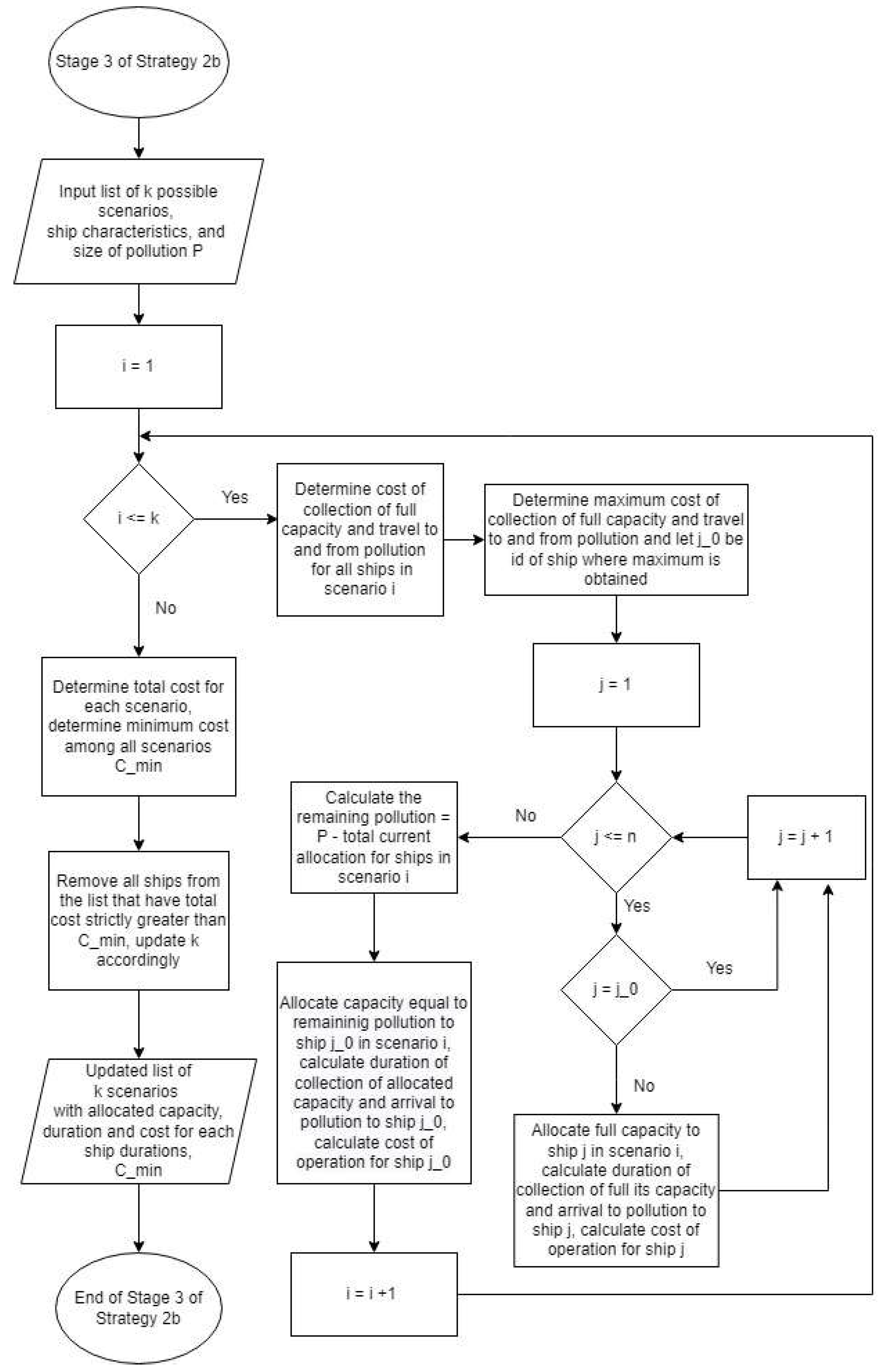
Algorithm A3: Strategy 2b
Input: Matrix of ship data A (A has n rows, where n is number of available ships; the columns are as follows: A[:, 1] (the first column of A)—ship capacity in m3; A[:, 2] (the second column of A)—oil collection rate in m3/h; A[:, 3] (the third column of A)—distance from pollution in km; A[:, 4] (the fourth column of A)—average sailing speed in km/h; A[:, 5] (the fifth column of A)—price of participation in the operation in EUR/h); volume of pollution: P in m3.
Output: Number of optimal scenarios k; matrix of optimal scenarios M (M has k rows and n columns; M[I,j]—quantity of pollution assigned to ship j in solution i), matrix of duration for each scenario: T (T has k rows and n columns, T[i,j]—duration of operation of ship j in scenario i); duration of operation: T_min, matrix of cost for each scenario: C (C has k rows and n columns, T[i,j]—cost of operation of ship j in scenario i); total cost of operation: C_min.
1Initialization: M is the matrix of all possible solutions (M has binary entries, 2n-1 rows and n columns, M[I,j] = 0 means that ship j is not assigned and M[i,j] = 1 means that ship j is assigned in the i-th solution.); k = 2n-1.
Stage 1: Elimination of scenarios with insufficient capacity
2for i = 1, 2,…, k do:
3      if the dot product of M[i, :] and A[:, 1] (the total capacity of ships in the i-th scenario) is less than P
4            Remove row i from matrix M      
5      end if
6end for
7k = number of rows of matrix M
Stage 2: Removing redundancies
8for i = 1, 2,…, k do:
9      d = elementwise product of M[i, :] and A[:, 0] in which all zeros have been removed capacity vector of ships in scenario i
10      d_min =min(d) … the minimum capacity of an individual ship in the scenario i
11      d_tot =min(d) … total capacity in the scenario i
12      if d_tot–d_min >= P
13            Remove row i from matrix M
14      end if
15end for
16k = number of rows of matrix M
Stage 3: Job allocation and cost minimization
17Initialization: T = kxn nul-matrix; C_min = 0, C = kxn nul-matrix
18for i = 1, 2, …, k
19      cap = elementwise product of A[:, 1] and M[i, :] … vector of maximum capacities of the i-th scenario
20      cap_tot =sum(cap) … total maximum capacity of the i-th scenario
21      a = elementwise quotient of A[:, 3], A[:,4] multiplied elementwise by M[i, :] … arrival duration vector for ships in scenario i
22      col = elementwise quotient of A[:, 1] and A[:, 2] multiplied elementwise with the M[i, :] … the duration vector of full capacity collection of all ships participating in the operation according to scenario i
23      cost = elementwise product of (a*2 + col) and A[:, 5] … total cost vector for ships in scenario i
24      j_0 = argmax(cost) … index corresponding to the vessel that has the largest individual total cost in i-th scenario
25      for j = 1, 2, …, n do:
26            if j≠ j_0      
27                  M[i, j] = cap[j] … Update the i-th row of the matrix M so that instead of each unit, except the one corresponding to the ship j_0, it is replaced with the maximum capacity of that ship.
28                  T[i, j] = a[j] + col[j] … Update the i-th row of the matrix T so that instead of each unit, except the one corresponding to the ship j_0, it is replaced with the total duration for that ship.
29                  C[i, j] = cost[j] … Update the i-th row of the matrix C so that instead of each unit, except the one corresponding to the ship j_0, it is replaced with the total cost for that ship.
30            otherwise if j = j_0
31                  M[i, j] = cap[j]–(cap_tot–P) … Update value in the i-th row of matrix M corresponding to ship j_0 with the remaining volume of pollution.
32                  T[i, j] = a[j] + M[i, j]/A[j, 2] … Update value in the i-th row of matrix T corresponding to ship j_0 with the duration of the arrival and collection of the allocated volume of pollution according to the corresponding value in the matrix M.
33                  C[i, j] = (T[i, j] + a[j]) * A[j, 5] … Update value in the i-th row of matrix C corresponding to ship j_0 with the total cost of arrival, departure and collection of the allocated volume of pollution according to the corresponding value in the matrix M.
34      end for
35      c =sum(T[i, :]) … total cost of the operation in scenario i
36      if i = 1
37            C_min = c
38      otherwise if C_min > c
39            C_min = c
40      end if
41for i = 1, 2,…, k do:
42      if C_min < sum(C[i, :])
43            Remove row i from matrix M
44            Remove row i from matrix T
45            Remove row i from matrix C
46      end if
47end for
48k = number of rows of matrix M      
Stage 4: Operation duration minimization
49Initialization: T_min = 0
50for i = 1, 2,…, k do:
51      t =max(T[i, :]) … duration of the operation in scenario i
52      if i = 1
53            T_min = t
54      otherwise if T_min > t
55            T_min = t
56      end if
57end for
58for i = 1, 2,…, k do:
59      if T_min < max(T[i, :])
60            Remove row i from matrix C
61            Remove row i from matrix M
62            Remove row i from matrix T
63      end if
64end for
65k = number of rows of matrix M

References

  1. Fratila, A.; Gavril, I.; Nita, S.; Hrebenciuc, A. The Importance of Maritime Transport for Economic Growth in the European Union: A Panel Data Analysis. Sustainability 2021, 13, 7961. [Google Scholar] [CrossRef]
  2. Zhang, Q.; Wen, Y.; Han, D.; Zhang, F.; Xiao, C. Construction of knowledge graph of maritime dangerous goods based on IMDG code. Int. J. Eng. Technol. 2020, 2020, 361–365. [Google Scholar] [CrossRef]
  3. Review of Maritime Transport. 2021. Available online: https://unctad.org/system/files/official-document/rmt2021_en_0.pdf (accessed on 11 February 2022).
  4. Jagerbrand, A.; Brutemark, A.; Sveden, J.; Gren, I. Review on the Environmental Impacts of Shipping on Aquatic and Nearshore Ecosystems. Sci. Total Environ. 2019, 695, 133637. [Google Scholar] [CrossRef] [PubMed]
  5. Protocol on Preparedness, Response and Co-Operation to Pollution Incidents by Hazardous and Noxious Substances. 2000. Available online: https://disasterlaw.ifrc.org/sites/default/files/media/disaster_law/2020-08/I627EN.pdf (accessed on 25 February 2022).
  6. EPA, Understanding Oil Spills and Oil Spill Response. Available online: https://www.epa.gov/sites/default/files/2018-01/documents/ospguide99.pdf (accessed on 3 April 2022).
  7. Lazuga, K.; Gucma, L.; Perkovic, M. The Model of Optimal Allocation of Maritime Oil Spill Combat Ships. Sustainability 2018, 10, 2321. [Google Scholar] [CrossRef] [Green Version]
  8. Dorčić, I. The Basic of Cleaning Oil Pollution, 1st ed.; INA Development and Research: Zagreb, Croatia, 1987; pp. 1–3. [Google Scholar]
  9. Dhaka, A.; Chattopadhyay, P. A Review on Physical Remediation Techniques for Treatment of Marine Oil Spills. J. Environ. Manag. 2021, 288, 112428. [Google Scholar] [CrossRef]
  10. Etkin, D.; Nedwed, T. Effectiveness of Mechanical Eecovery for Large Offshore oil spills. Mar. Pollut. Bull. 2021, 163, 111848. [Google Scholar] [CrossRef]
  11. Vetere, A.; Profrock, D.; Schrade, W. Qualitative and Quantitative Evaluation of Sulfur-Containing Compound Types in Heavy Crude Oil and its Fractions. Energy Fuels 2021, 35, 8723–8732. [Google Scholar] [CrossRef]
  12. IMO Model Courses–First Responders. Available online: https://www.imo.org/en/OurWork/Environment/Pages/IMO-OPRC-Model-Courses.aspx (accessed on 10 April 2022).
  13. Weiwei, J.; Wei, A.; Yupeng, Z.; Zhaoyu, Q. Research on Scheduling Optimization of Marine Oil Spill Emergency Vessels. Aquat. Procedia 2015, 3, 35–40. [Google Scholar] [CrossRef]
  14. Li, S.; Grifoll, M.; Estrada, M.; Zheng, P.; Feng, H. Optimization on Emergency Materials Dispatching Considering the Characteristics of Integraded Emergency Response for Large-Scale Marine Oil Spills. J. Mar. Sci. Eng. 2019, 7, 214. [Google Scholar] [CrossRef] [Green Version]
  15. Ye, X.; Chen, B.; Li, P.; Jing, L.; Zeng, G. A Simulations-based Multi-agent Particle Swarm Optimization Approach for Supporting Dynamic Decision Making in Marine Oil Spill Response. Ocean Coast. Manag. 2019, 172, 128–136. [Google Scholar] [CrossRef]
  16. Ye, X.; Chen, B.; Lee, K.; Storesund, R.; Li, P.; Kang, Q. An Emergency Response System by Dynamic Simulation and Enhanced Particle Swarm Optimization and Application for a Marine Oil Spill Accident. J. Clean. Prod. 2021, 287, 126591. [Google Scholar] [CrossRef]
  17. Tijan, E.; Jović, M.; Aksentijević, S.; Pucihar, A. Digital Transformation in the Maritime Transport Sector. Technol. Forecast. Soc. Change. 2021, 170, 120879. [Google Scholar] [CrossRef]
  18. Peša, I.; Ross, C. Extractive Industries and the Environment: Production, Pollution, and Protest in Global History. Extr. Ind. Soc. 2021, 8, 100933. [Google Scholar] [CrossRef]
  19. Fingas, M. Remote Sensing for Marine Management. In World Seas: An Environmental Evaluation, 2nd ed.; Ecological Issues and Environmental Impacts; Elsevier: Amsterdam, The Netherlands, 2019; Volume 3, pp. 103–119. [Google Scholar]
  20. Keramea, P.; Kokkos, N.; Gikas, G.; Sylaios, G. Operational Modeling of North Aegean Oil Spills Forced by Real-Time Met-Ocen Forecast. J. Mar. Sci. Eng. 2022, 10, 411. [Google Scholar] [CrossRef]
  21. Zerebecki, R.; Heck, K.; Valentine, J. Biodiversity Influences the Effects of Oil Disturbance on Coastal Ecosystems. Ecol. Evol. 2022, 12, 23–28. [Google Scholar] [CrossRef]
  22. ITOPF. Available online: https://www.itopf.org/knowledge-resources/data-statistics/statistics/ (accessed on 14 April 2022).
  23. Ulker, D.; Burak, S.; Balas, L.; Caglar, N. Mathematical Modeling of Oil Spill Weathering Processes for Contingency Planning in Izmit Bay. Reg. Stud. Mar. Sci. 2022, 50, 102155. [Google Scholar] [CrossRef]
  24. Silva, I.A.; Almeida, F.C.; Souza, T.C.; Bezerra, K.G.; Durval, I.J.; Converti, A.; Sarubbo, L.A. Oil Spills: Impacts and Perspectives of Treatment Technologies with Focus on the Use of Green Surfactants. Environ Monit Assess. 2022, 194, 143. [Google Scholar] [CrossRef]
  25. Cano, J.; Loza, J.; Guida, P.; Roberts, W.; Chejne, F.; Sarathy, S.; Im, G. Evaporation, break-up, and Pyrolysis of Multicomponent Arabian Light Crude Oil Droplets at Various Temperatures. Int. J. Heat Mass Transf. 2022, 183, 103–106. [Google Scholar]
  26. Majid, D.; Farahani, D.; Zheng, Y. The Formulation, Development and Application of Oil Dispersants. J. Mar. Sci. Eng. 2022, 10, 425. [Google Scholar]
  27. Alade, I.; Oyedeji, M.; Rahman, M.; Saleh, T. Predicting the Density of Carbon-based Nanomaterials in Diesel Oil Through Computational Intelligence Methods. J. Therm. Anal. Calorim. 2022, 10, 425. [Google Scholar] [CrossRef]
  28. Gao, X.; Dong, P.; Cui, J.; Gao, Q. Prediction Model for the Viscosity of Heavy Oil Diluted with Light Oil Using Machine Learning Techniques. Energies 2022, 15, 2297. [Google Scholar] [CrossRef]
  29. Krivoshchekov, S.; Kochnev, A.; Vyatkin, K. The Development of Forecasting Technique for Cyclic Steam Stimulation Technology Effectiveness in Near–Wellbore Area. Fluids 2022, 7, 64. [Google Scholar] [CrossRef]
  30. Chacon-Patino, M.; Nelson, J.; Rogel, E.; Hench, K.; Poirier, L.; Lopez-Linares, F.; Ovalles, C. Vanadium and Nickel Distributions in Selective-separated n-heptane Asphaltenes of Heavy Crude Oils. Fuel 2022, 312, 23–28. [Google Scholar] [CrossRef]
  31. El-Gayar, D.; Khodary, M.; Abdel-Aziz, H.; Khalil, M. Effect of Disk Skimmer Material and Oil Viscosity on Oil Spill Recovery. Water Air Soil Pollut. 2021, 232, 193. [Google Scholar] [CrossRef]
  32. Salma Rima, U.; Beier, N. Effects of Seasonal Weathering on Dewatering and Strength of an Oil Sands Tailings Deposit. Can. Geotech. J. 2022, 59, 145–151. [Google Scholar]
  33. Bacosa, H.; Ancla, S.; Loui, C.; Russel, J. From Surface Water to the Deep Sea: A Review on Factors Affecting the Biodegradation of Spilled Oil in Marine Environment. J. Mar. Sci. Eng. 2022, 10, 426. [Google Scholar] [CrossRef]
  34. Hass Freeman, D.; Ward, C. Sunlight-driven Dissolution is a Major Fate of Oil at Sea. Sci. Adv. 2022, 8, 42–43. [Google Scholar] [CrossRef]
  35. Allahabady, A.; Yousefi, Z.; Tahamtan, R.; Sharif, Z. Measurement of BTEX (Benzene, Toluene, Ethylbenzene and Xylene) Concertation at Gas Stations. Environ. Eng. Manag. J. 2022, 9, 23–31. [Google Scholar]
  36. You, Y.; Liu, C.; Hu, Q.; Zhang, S.; Wang, C. Response Surface Methodology to Optimize Ultrasonic-Assisted Extraction of Crude Oil from Oily Sludge. Pet. Sci. Technol. 2022, 40, 15–18. [Google Scholar] [CrossRef]
  37. Yamada, K.; Yagishita, K.; Sato, K. Dispersion States of Lecithin-Soybean Oil Mixtures in Water. Colloid. Polym. Sci. 2022, 300, 95–102. [Google Scholar] [CrossRef]
  38. Zhang, X.; Ni, W.; Sun, L. Fatigue Analysis of the Oil Offloading Lines in FPSO System Under Wave and Current Loads. J. Mar. Sci. Eng. 2022, 10, 225. [Google Scholar] [CrossRef]
  39. Manivel, R.; Sivakumar, R. Boat Type Oil Recovery Skimmers. Mater. Today Proc. 2020, 21, 470–473. [Google Scholar] [CrossRef]
  40. Song, J.; Lu, Y.; Luo, J.; Huang, S.; Wang, L.; Xu, W.; Parkin, I.P. Barrel-Shaped Oil Skimmer Designed for Collection of Oil from Spills. Adv. Mater. Interfaces 2015, 2, 1500350. [Google Scholar] [CrossRef]
  41. Herbst, L. Fishing for Oil. IEEE Spectr. 2020, 57, 36–50. [Google Scholar] [CrossRef]
  42. Revollo, N.; Delrieux, A. Vessel and Oil Spill Early Detection Using COSMO Satellite Imagery. SPIE Remote Sens. 2017, 2017, 1042203. [Google Scholar]
  43. Fedrizzia, T.; Ciania, Y.; Lorenzina, F.; Cantorea, T.; Gasperinia, P.; Demichelis, F. Fast Mutual Exclusivity Algorithm Nominates Potential Synthetic Lethal Gene Pairs Through Brute Force Matrix Product Computations. Comput. Struct. Biotechnol. J. 2021, 19, 4394–4403. [Google Scholar] [CrossRef]
Figure 1. Number of medium and large tanker spills per year from 1970 to 2021. Reproduced with permission from ITOPF, 2022 [22].
Jmse 10 00772 g001
Figure 2. Changes in oil (Arabian extra light (Aramco)) density over time on the surface of water (from the ADIOS program).
Jmse 10 00772 g002
Figure 3. Changes in oil (Arabian extra light (Aramco)) viscosity over time on the surface of water (from the ADIOS program).
Jmse 10 00772 g003
Figure 4. Oil budget: A view of an ADIOS spill scenario, showing remaining, dispersed, and evaporated oil (Arabian extra light (Aramco)) over time (from the ADIOS program).
Jmse 10 00772 g004
Figure 5. Flowchart for Stage 1.
Jmse 10 00772 g005
Figure 6. Flowchart for Stage 2 of Strategies 2a and 2b.
Jmse 10 00772 g006
Figure 7. General flowchart for all strategies. S can be Strategy 1, 2a, or 2b.
Jmse 10 00772 g007
Figure 8. Flowchart for Stage 2 of Strategy 1.
Jmse 10 00772 g008
Figure 9. Flowchart for Stage 3 of Strategy 1.
Jmse 10 00772 g009
Figure 10. Flowchart for Stage 4 of Strategy 1.
Jmse 10 00772 g010
Figure 11. Flowchart for Stage 3 of Strategy 2a.
Jmse 10 00772 g011
Figure 12. Flowchart for Stage 4 of Strategy 2a.
Jmse 10 00772 g012
Figure 13. Flowchart for Stage 3 of Strategy 2b.
Jmse 10 00772 g013
Figure 14. Flowchart of Stage 4 of Strategy 2b.
Jmse 10 00772 g014
Table 1. Order of optimization criteria for different versions of Strategy 2.
Order of CriteriaStrategy 2aStrategy 2b
1.Minimum total durationMinimum cost
2.Minimum costMinimum total duration
Table 2. Example 1—input data.
Ship IDShip Capacity (m3)Oil Collection Rate (m3/h)
1101
2121
3161
4201
Table 3. Example 1—output of Stage 1.
Ship ID1234
Scenario
10011
20101
30110
40111
51001
61010
71011
81101
91110
101111
Table 4. Example 1—output of Stage 2.
Ship ID1234
Scenario
10011
20101
30110
51001
61010
Table 5. Example 1—final results of the allocation (m3).
Ship ID1234
Scenario
100169
2012013
3012130
5100015
6100150
Table 6. Example 1—final results of the duration (h).
Ship ID1234
Scenario
100169
2012013
3012130
5100015
6100150
Table 7. Example 2—input data. The price (EUR/h*) is hypothetical.
Ship IDShip Capacity (m3)Oil Collection Rate (m3/h)Distance From Pollution (km)Average Sailing Speed (km/h)Price of Participation in the Operation (EUR/h*)
1101111
2121112
3161111
4201111
Table 8. Example 2—all possible scenarios.
Ship ID 1234
Scenario
10011
20101
30110
40111
51001
61010
71011
81101
91110
101111
Table 9. Example 2—results after Stage 2.
Ship ID1234
Scenario
10011
20101
30110
51001
61010
Table 10. Example 2—final allocation for Strategy 2a (m3).
Ship ID1234
Scenario
2012013
3012130
Table 11. Example 2—final duration for Strategy 2a (h).
Ship ID 1 2 3 4
Scenario
2013014
3013140
Table 12. Example 2—final cost for Strategy 2a (EUR).
Ship ID1234
Scenario
2028015
3028150
Table 13. Example 2—final allocation for Strategy 2b (m3).
Ship ID1234
Scenario
100169
5100015
6100150
Table 14. Example 2—final duration for Strategy 2b (h).
Ship ID1234
Scenario
1001710
5110016
6110160
Table 15. Example 2—final cost for Strategy 2b (EUR).
Ship ID1234
Scenario
1001811
5120017
6120170
Table 16. Example 3—input data.
Ship IDShip Capacity (m3)Oil Collection Rate (m3/h)Distance from Pollution (km)Average Sailing Speed (km/h)Price of Participation in the Operation (EUR/h)
EKO 20001061018.52500
EKO 1 20001061518.52500
Publisher’s Note: MDPI stays neutral with regard to jurisdictional claims in published maps and institutional affiliations.

