
Hydrodynamic Forces and Wake Distribution of Various Ship Shapes Calculated Using a Reynolds Stress Model


Abstract
:1. Introduction
2. Validation of Turbulence Models
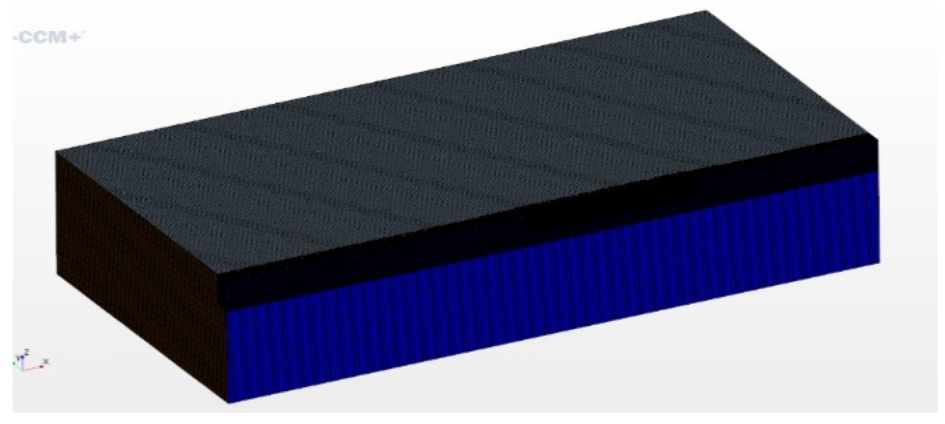
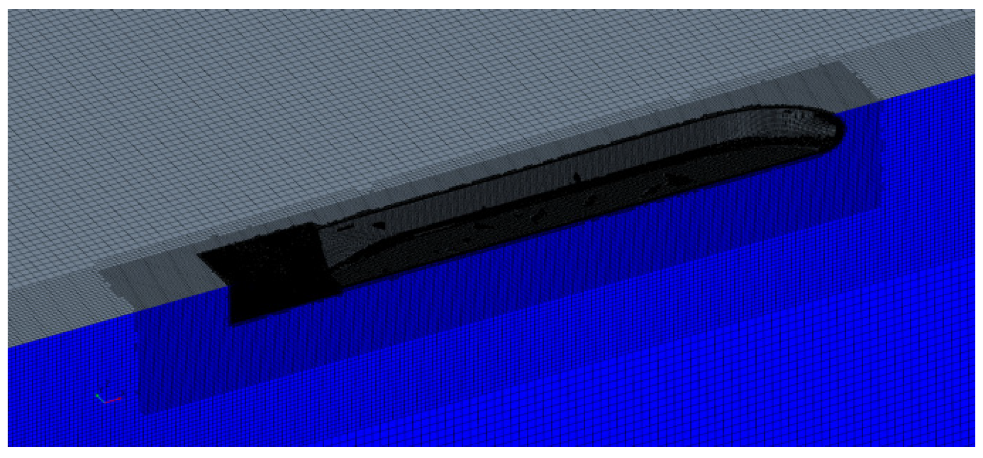
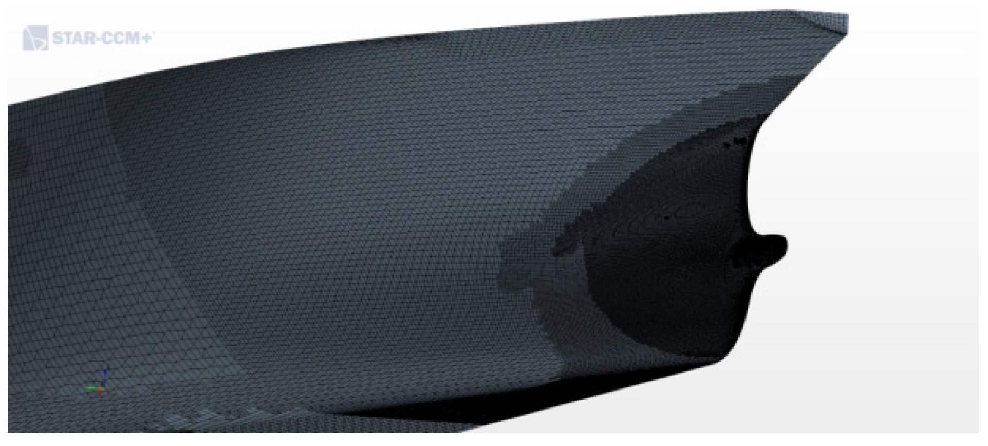
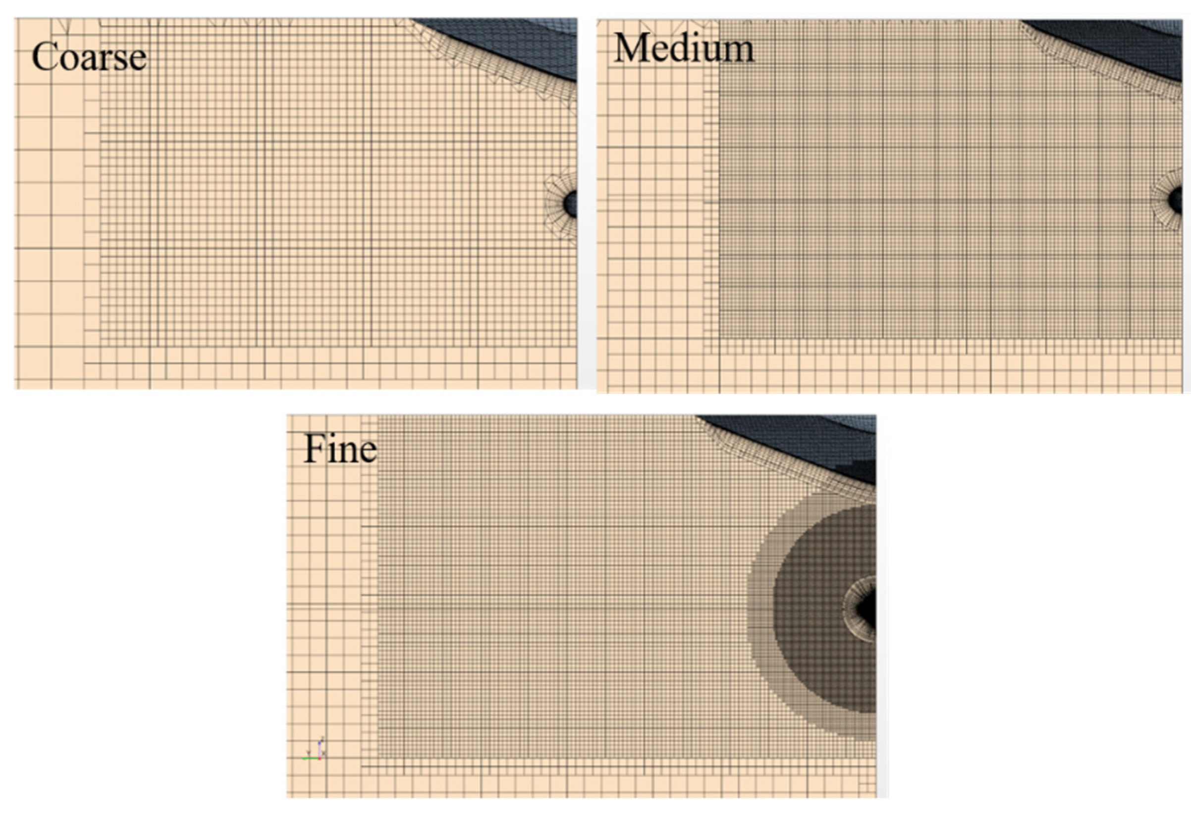
2.1. Computational Conditions
2.2. Verification and Validation (V&V) Method
- (i)
- Monotonic convergence: 0 < R < 1;
- (ii)
- Oscillatory convergence: R < 0;
- (iii)
- Divergence: R > 1.
2.3. Results of the Verification and Validation
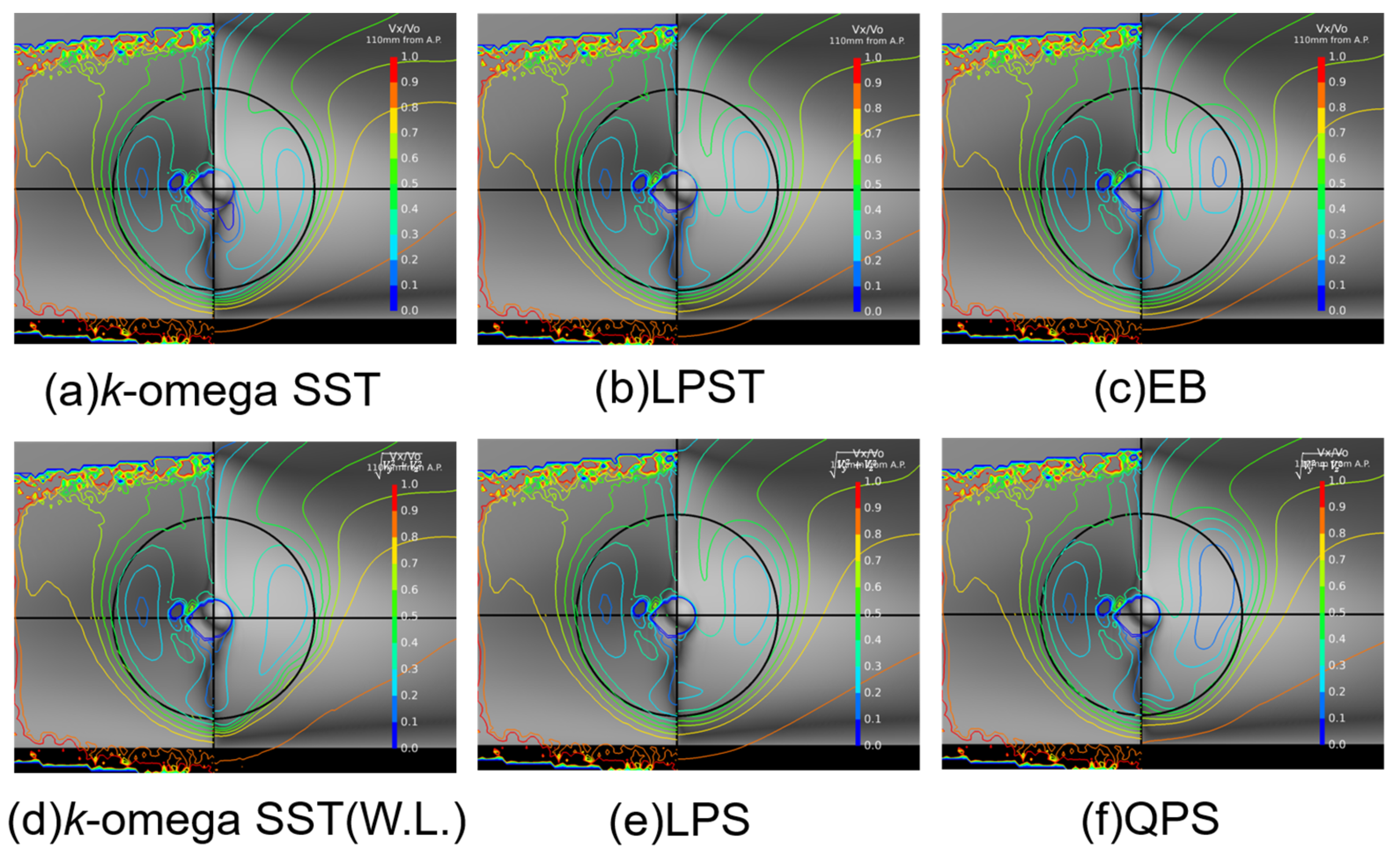
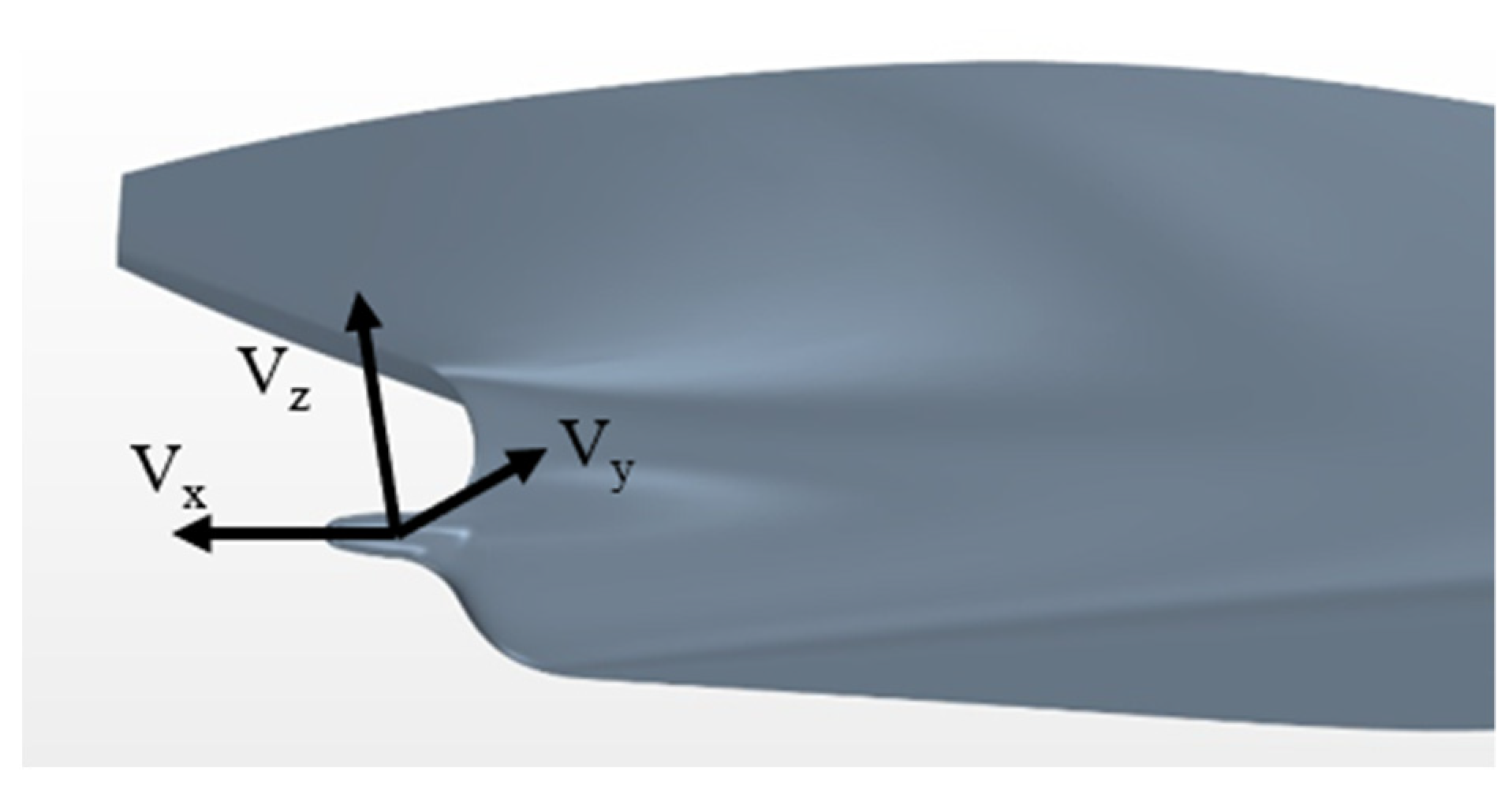
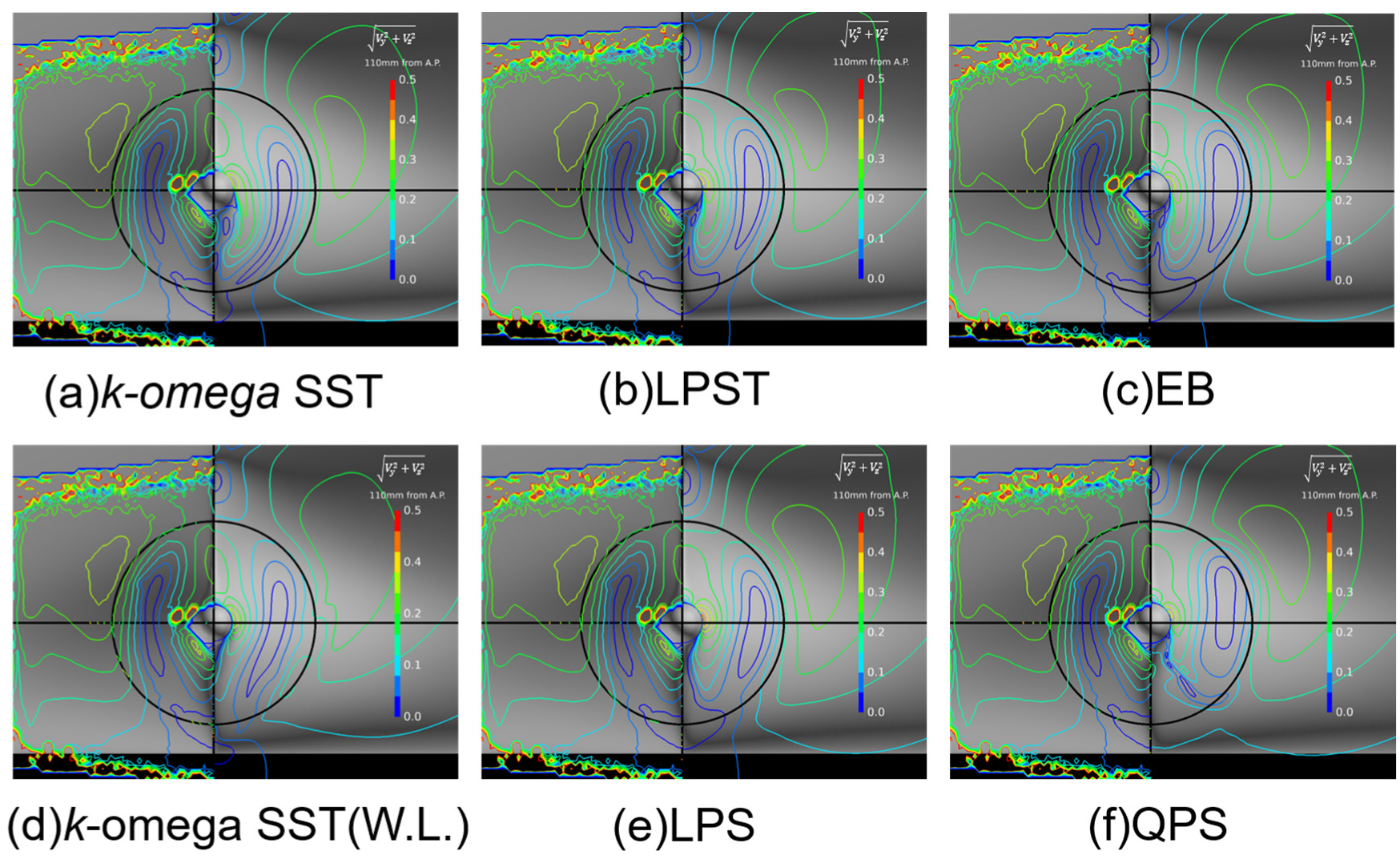
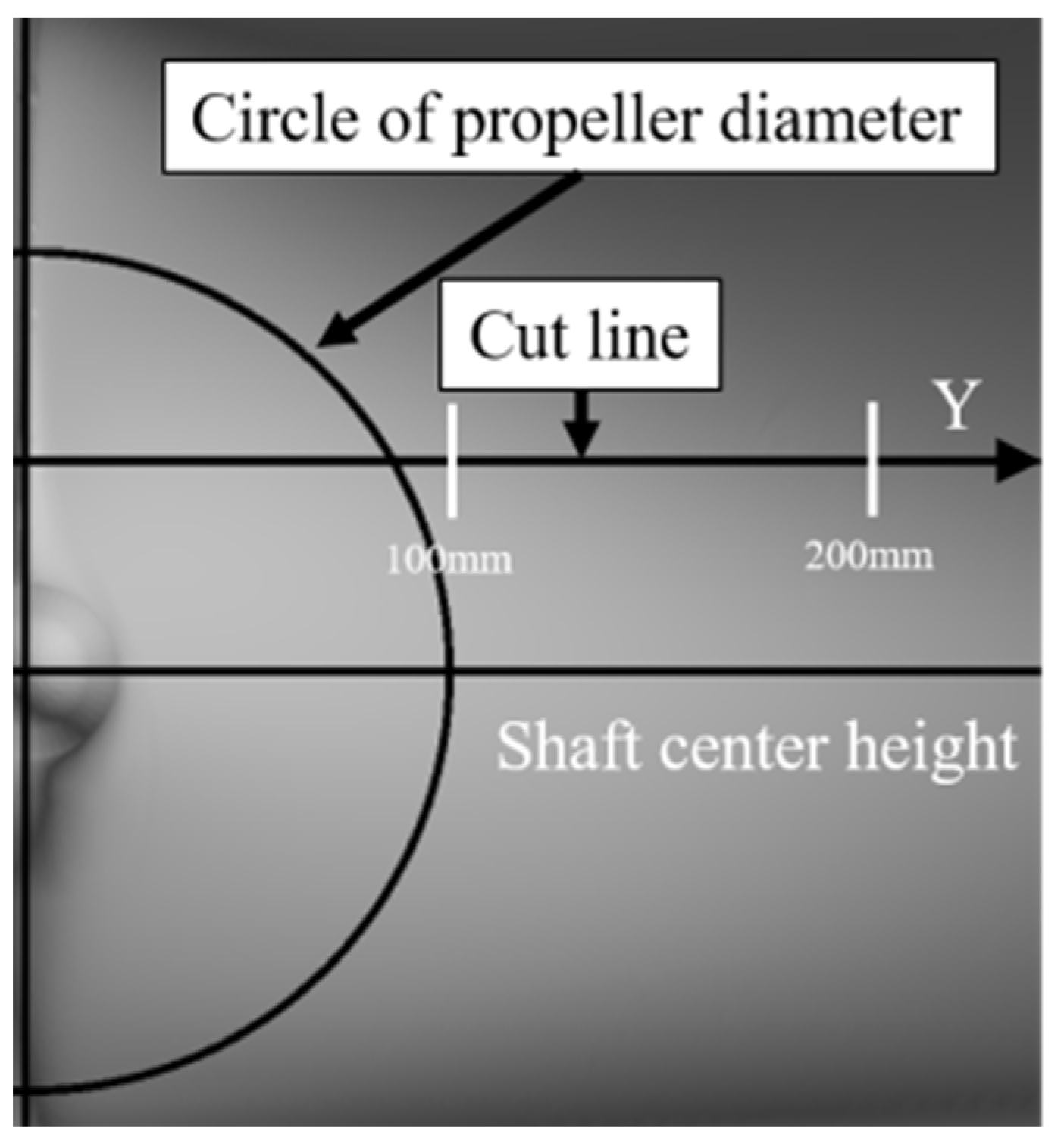
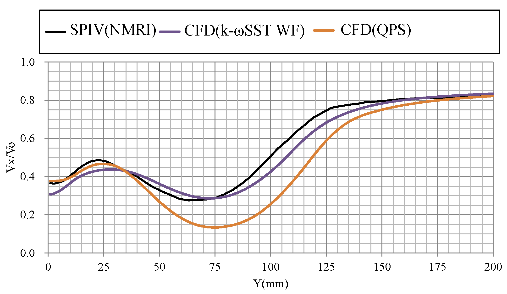
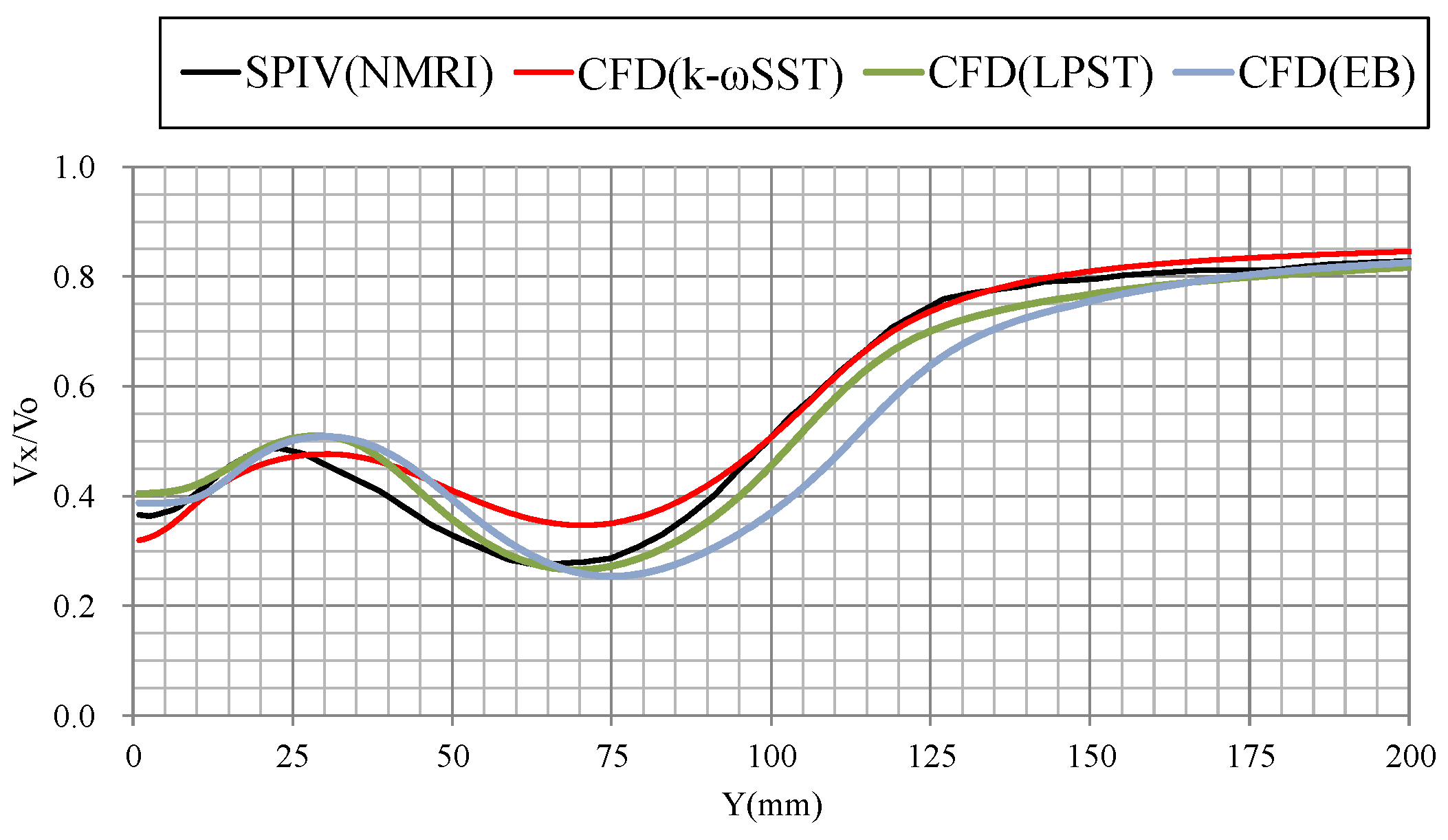
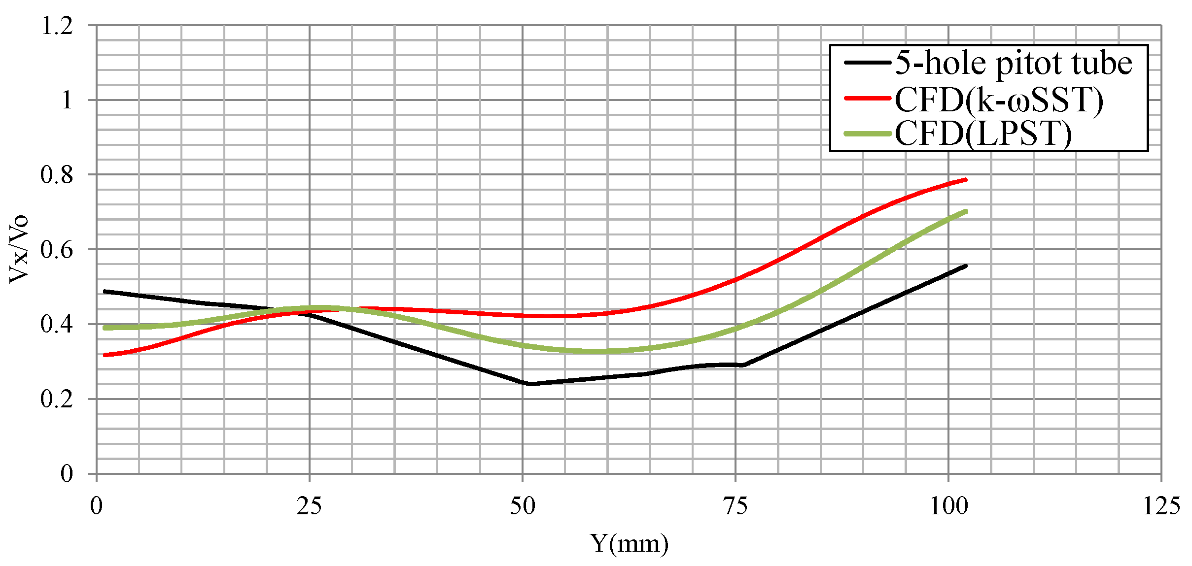
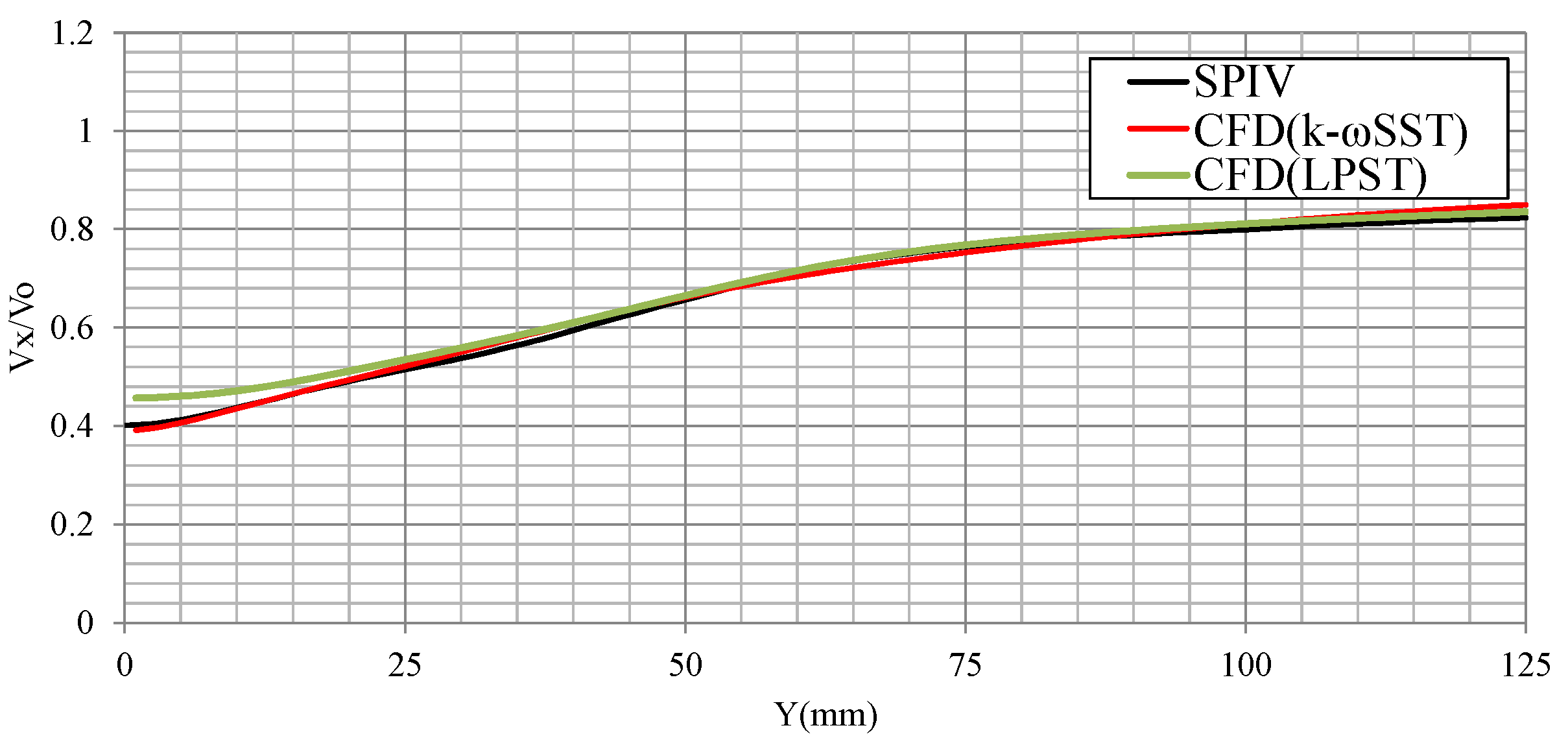
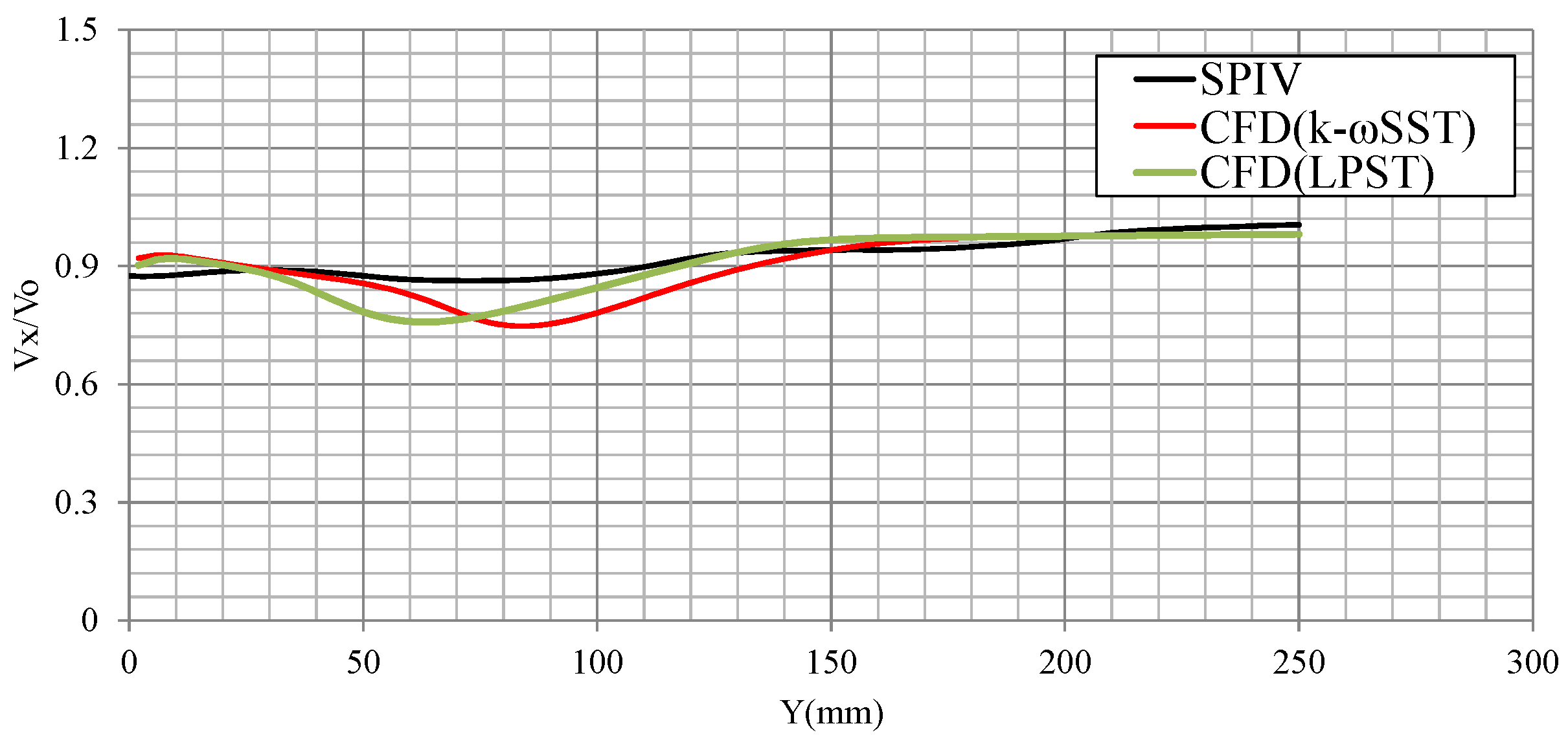
2.4. Validation of the Wake Distribution
3. Validation of the Calculation Results of the k–Omega SST Model and the RSM, Depending on the Ship Type
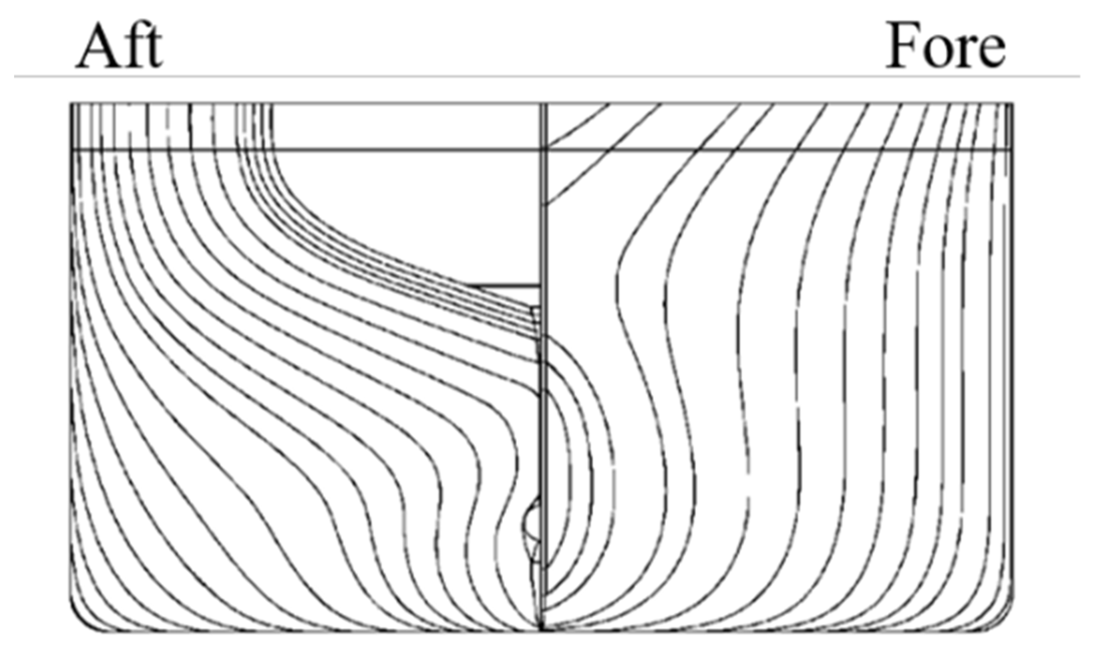
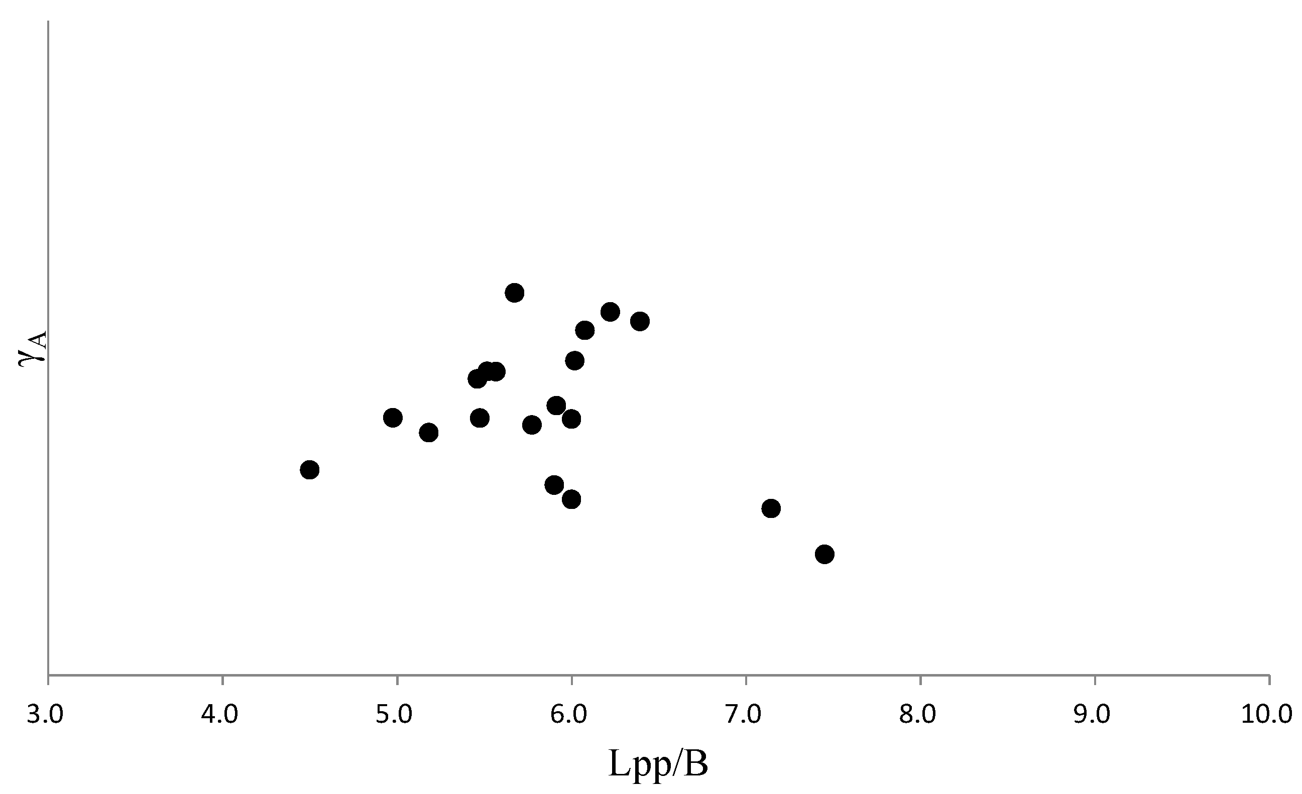
3.1. Ship Types Used in the Calculations
3.2. Result of the CFD Calculation
4. Conclusions
- The calculated numerical uncertainty of the k–omega SST model without a wall function is lower than that of the other turbulence models. Therefore, the k–omega SST model without a wall function shows less grid dependency in the calculation of viscous resistance compared with the other turbulence models.
- The RSM shows a numerical uncertainty (approximately 0.25%) higher than that of the k–omega SST model. However, its uncertainty is generally smaller than that obtained from experiments. Nevertheless, the RSM is a promising turbulence model with low numerical uncertainty.
- The comparison error of the k–omega SST model is much larger than the validation uncertainty . Therefore, the turbulence model needs to be improved. Meanwhile, the of the LPS and LPST models is much less than . Thus, this turbulence model is accurate since it produces results similar to those obtained from experiments.
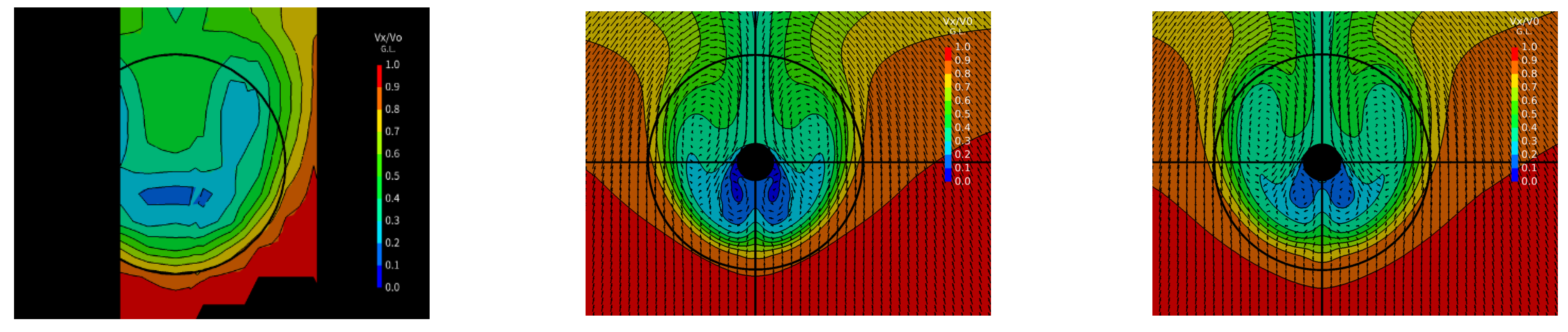
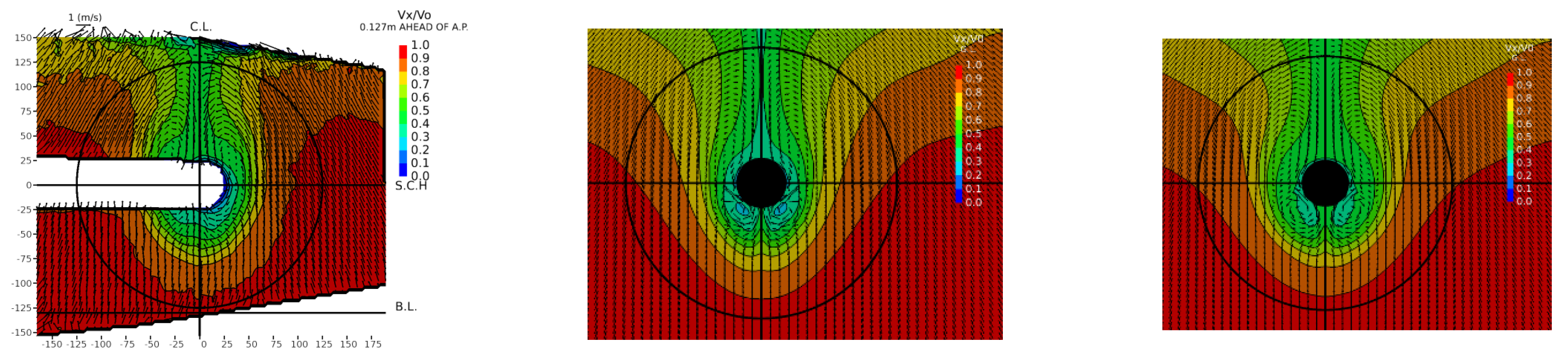
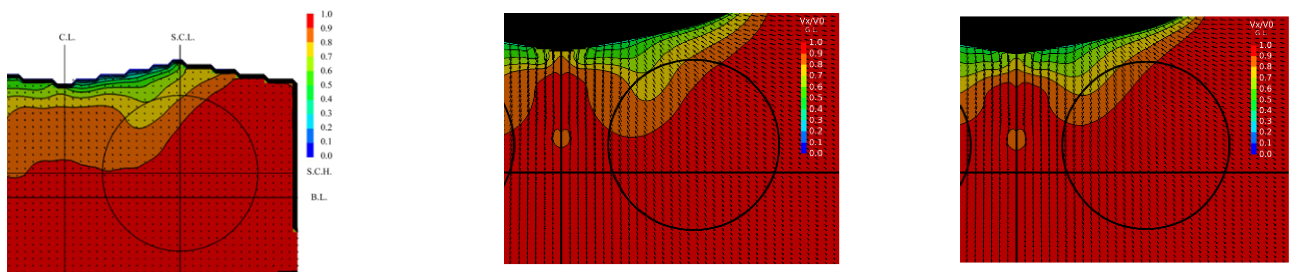
- The calculated wake distributions using RSMs exhibit good agreement with SPIV measurements, except for the QPS model. Specifically, using the LPS and LPST models, the size of the stern longitudinal vortex and the wake distribution under the shaft can be estimated with high accuracy.
- The LPST model is capable of estimating the axial velocity distribution along the horizontal line above the propeller shaft with high accuracy. If the vortex core can be estimated accurately, it will be possible to design a wake-adapted propeller with high accuracy.
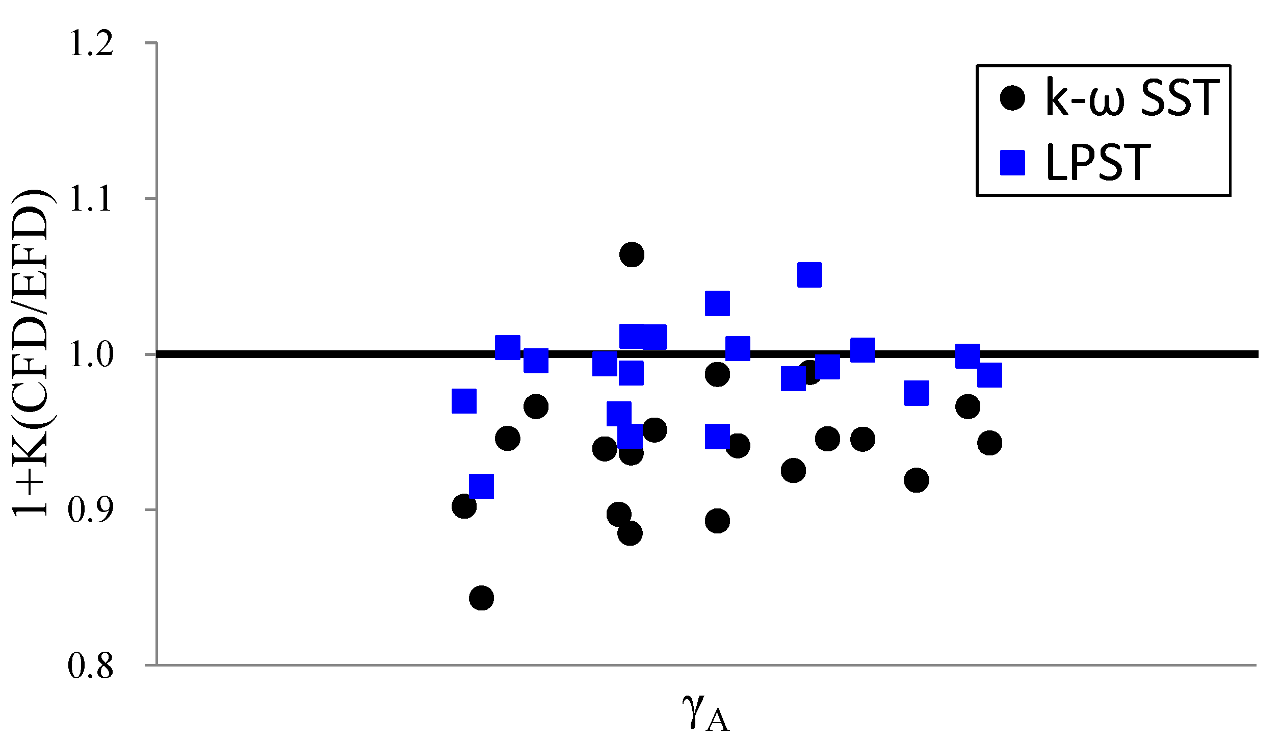
- The LPST shows a small difference between the EFD and CFD calculations. The standard error SE of the LPST model is smaller than the SE of the k–omega SST model. Therefore, the LPST model is capable of estimating the viscous resistance with high accuracy in our setting.
- The calculation results obtained using the KVLCC2 model show the same trend as those of a JBC hull form. Moreover, it is clear that the LPST model is capable of accurately estimating the stern longitudinal vortex hooks.
- The calculation results of the KCS and Model 5415 show that there is almost no difference from those produced by the k–omega SST and LPST models. Therefore, it was confirmed that the k–omega SST model is capable of efficiently estimating the and wake distribution of fine hull–forms.
Author Contributions
Funding
Conflicts of Interest
References
- IMO, MEPC. Guide Lines on Survey and Certificaion of the Energy Efficiency Design Index (EEDI). MEPC 63/23/Add.1 Annex 10. 2012. Available online: https://wwwcdn.imo.org/localresources/en/OurWork/Environment/Documents/214(63).pdf (accessed on 1 February 2020).
- IMO, MEPC. Initial Imo Strategy on Reduction of Ghg Emissions From Ships. MEPC 72/17/Add.1 Annex 11. 2018. Available online: https://wwwcdn.imo.org/localresources/en/OurWork/Environment/Documents/ResolutionMEPC.304(72)_E.pdf (accessed on 1 February 2020).
- Su, Y.; Lin, J.; Zhao, D.; Guo, C.; Guo, H. Influence of a pre-swirl stator and rudder bulb system on the propulsion performance of a large-scale ship model. Ocean Eng. 2020, 218, 108189. [Google Scholar] [CrossRef]
- Pena, B.; Luofeng, H. A review on the turbulence modelling strategy for ship hydrodynamic simulations. Ocean Eng. 2021, 241, 110082. [Google Scholar] [CrossRef]
- Webpage, Tokyo 2015 a Workshop on CFD in Ship Hydrodynamics. 2015. NMRI. Available online: http://www.t2015.nmri.go.jp/index.html (accessed on 1 February 2020).
- Terziev, M.; Tezdogan, T.; Incecik, A. Application of Eddy-Viscosity Turbulence Models to Problems in Ship Hydrodynamics. In Ships and Offshore Structures; Taylor & Francis: Oxfordshire, UK, 2020; Volume 15. [Google Scholar]
- Visonneau, M.; Deng, G.; Queutey, P.; Guilmineau, E.; del Toro Llorens, A. High-Fidelity Computational Analysis of an Energy-Saving Device at Model-scale. In Proceedings of the Hull Performance & Insight Conference (HullPIC), Turin, Italy, 13–15 April 2016. [Google Scholar]
- Gaggero, S.; Villa, D.; Viviani, M. An extensive analysis of numerical ship self-propulsion prediction via a coupled BEM/RANS approach. Appl. Ocean Res. 2017, 66, 55–78. [Google Scholar] [CrossRef]
- Andrea, F.; Nastia, D.; Ivana, M.; Roko, D. Numerical and experimental assessment of nominal wake for a bulk carrier. J. Mar. Sci. Technol. 2019, 24, 1092–1104. [Google Scholar]
- Tatsuo, N.; Yoshinobu, Y.; Masaru, S.; Chisachi, K. Application of Fully-resolved Large Eddy Simulation to KVLCC2 –Bare Hull Double Model at Model Ship Reynolds Number. J. Jpn. Soc. Nav. Archit. Ocean. Eng. 2012, 16, 1–9. [Google Scholar]
- Kornev, N.; Abbas, N. Vorticity structures and turbulence in the wake of full block ships. J. Mar. Sci. Technol. 2018, 23, 567–579. [Google Scholar] [CrossRef]
- Liefvendahl, M.; Johansson, M. Wall-modeled LES for ship hydrodynamics in model-scale. J. Ship Res. 2021, 65, 41–54. [Google Scholar] [CrossRef]
- Stern, F.; Wilson, R.V.; Coleman, H.W.; Paterson, E.G. Verification and Validation of CFD Simulations; IIHR Report No. 407; Iowa Institute of Hydraulic Research College of Engineering, The University of Iowa: Iowa City, IA, USA, 1999. [Google Scholar]
- Menter, F.R. Two-Equation Eddy-Viscosity Turbulence Models for Engineering Applications. AIAA J. 1994, 32, 1598–1605. [Google Scholar] [CrossRef] [Green Version]
- Gibson, M.M.; Launder, B.E. Ground effects on pressure fluctuations in the atmospheric boundary layer. J. Fluid Mech. 1978, 86, 491–511. [Google Scholar] [CrossRef]
- Rodi, W. Experience with Two-Layer Models Combining the k-e Model with a One-Equation Model Near the Wall. In Proceedings of the 29th Aerospace Sciences Meeting, AIAA 91-0216, Reno, NV, USA, 7–10 January 1991. [Google Scholar]
- Launder, B.E.; Shima, N. Second Moment Closure for the Near-Wall Sublayer. Dev. Appl. AIAA J. 1989, 27, 1319–1325. [Google Scholar] [CrossRef]
- Speziale, C.G.; Sarkar, S.; Gatski, T.B. Modelling the pressure-strain correlation of turbulence: An invariant dynamical systems approach. J. Fluid Mech. 1991, 227, 245–272. [Google Scholar] [CrossRef]
- Manceau, R.; Hanjalic, K. Elliptic blending model: A new near-wall Reynolds-stress turbulence closure. Phys. Fluids 2002, 14, 744–764. [Google Scholar] [CrossRef]
- Lardeau, S.; Manceau, R. Computations of Complex Flow Configurations Using a Modified Elliptic-Blending Reynolds-Stress Model. In Proceedings of the 10th Engineering Turbulence Modelling and Experiments, Modelling and Measurement Conference, Marbella, Spain, 17–19 September 2014. [Google Scholar]
- ITTC. ITTC Recommended Procedures and Guidelines—Uncertainty Analysis in CFD Verification and Validation Methodology and Procedures., Approved 28th ITTC 2017, 09/2017. Available online: https://www.ittc.info/media/8153/75-03-01-01.pdf (accessed on 1 February 2020).
- Webpage, SIMMAN 2008. Available online: http://www.simman2008.dk/ (accessed on 1 February 2020).
- Lee, S.-J.; Kim, H.-R.; Kim, W.-J.; Van, S.-H. Wind tunnel tests on flow characteristics of the KRISO 3600 TEU containership and 300K VLCC double-deck ship models. J. Ship Res. 2003, 47, 24–38. [Google Scholar] [CrossRef]


| SHIP NAME | JBC | ||
|---|---|---|---|
| Model/Ship | Ship | Model | |
| Length between perpendiculars | Lpp (m) | 280.00 | 7.0000 |
| Length on waterline | LDwl (m) | 285.00 | 7.1250 |
| Breath | B (m) | 45.00 | 1.1250 |
| Depth | D (m) | 25.00 | 0.6250 |
| Draft | d(m) | 16.50 | 0.4125 |
| Block coefficient | Cb | 0.8580 | |
| Fn | 0.142 |
| Vm(m/s) | 1.179 |
| ρ(kg/m3) | 998.7 |
| ν × 10−6(m2/s) | 1.0789 |
| Rn | 7.649 × 10⁶ |
| W.o.W.F. | W.F. | ||
|---|---|---|---|
| Fine | NC1 | 16,179,979 | 14,762,102 |
| Midium | NC2 | 5,723,952 | 5,146,544 |
| Coarse | NC3 | 1,728,686 | 1,475,687 |
| r | 1.452 | 1.469 | |
| r21 | 1.414 | 1.421 | |
| r32 | 1.490 | 1.516 |
| R | p | δRE | C | δfine(%(1 + K)fine) | USN(%(1 + K)fine) | |||
|---|---|---|---|---|---|---|---|---|
| k-ω SST | 0.00091 | 0.13233 | 0.0068 | 13.361 | 6.236 × 10⁻⁶ | 130.910 | 0.07% | 0.13% |
| k-ω SST w.W.F. | −0.00024 | 0.01456 | −0.0166 | - | - | - | - | 0.55% |
| LPS | 0.00165 | 0.01056 | 0.1560 | 4.835 | 3.045 × 10⁻⁴ | 4.678 | 0.11% | 0.19% |
| LPST | 0.00206 | 0.01126 | 0.1832 | 4.549 | 4.625 × 10⁻⁴ | 4.021 | 0.14% | 0.25% |
| QPS | −0.00248 | 0.01076 | −0.2303 | - | - | - | - | 0.32% |
| EB | 0.00230 | 0.01086 | 0.2122 | 4.155 | 6.207 × 10⁻⁴ | 3.348 | 0.15% | 0.26% |
| E(%D) | UD(%D) | UV(%D) | EC(%D) | |
|---|---|---|---|---|
| k-ω SST | 4.65% | 1.0% | 1.01% | 4.72% |
| k-ω SST w.W.F. | 2.15% | 1.0% | 1.14% | - |
| LPS | −1.40% | 1.0% | 1.02% | −1.29% |
| LPST | −0.02% | 1.0% | 1.03% | 0.13% |
| QPS | 0.10% | 1.0% | 1.05% | - |
| EB | −6.57% | 1.0% | 1.04% | −6.41% |
| No. | Name | Rn |
|---|---|---|
| 1 | Ship A | 9.79 × 10⁶ |
| 2 | Ship B | 7.93 × 10⁶ |
| 3 | Model5415 | 5.72 × 10⁶ |
| 4 | Ship C | 4.37 × 10⁶ |
| 5 | Ship E | 7.13 × 10⁶ |
| 6 | JBC | 6.73 × 10⁶ |
| 7 | Ship F | 7.86 × 10⁶ |
| 8 | Ship G | 8.80 × 10⁶ |
| 9 | Ship H | 8.70 × 10⁶ |
| 10 | Ship I | 7.45 × 10⁶ |
| 11 | Ship J | 1.04 × 10⁶ |
| 12 | Ship K | 8.31 × 10⁶ |
| 13 | Ship L | 1.15 × 10⁷ |
| 14 | Ship M | 7.66 × 10⁶ |
| 15 | Ship N | 8.98 × 10⁶ |
| 16 | KCS | 1.30 × 10⁷ |
| 17 | KVLCC | 6.37 × 10⁶ |
| 18 | Ship O | 6.68 × 10⁶ |
| 19 | Ship P | 7.37 × 10⁶ |
| 20 | Ship Q | 7.28 × 10⁶ |
Publisher’s Note: MDPI stays neutral with regard to jurisdictional claims in published maps and institutional affiliations. |
© 2022 by the authors. Licensee MDPI, Basel, Switzerland. This article is an open access article distributed under the terms and conditions of the Creative Commons Attribution (CC BY) license (https://creativecommons.org/licenses/by/4.0/).
Share and Cite
Matsuda, S.; Katsui, T. Hydrodynamic Forces and Wake Distribution of Various Ship Shapes Calculated Using a Reynolds Stress Model. J. Mar. Sci. Eng. 2022, 10, 777. https://doi.org/10.3390/jmse10060777
Matsuda S, Katsui T. Hydrodynamic Forces and Wake Distribution of Various Ship Shapes Calculated Using a Reynolds Stress Model. Journal of Marine Science and Engineering. 2022; 10(6):777. https://doi.org/10.3390/jmse10060777
Chicago/Turabian StyleMatsuda, Satoshi, and Tokihiro Katsui. 2022. "Hydrodynamic Forces and Wake Distribution of Various Ship Shapes Calculated Using a Reynolds Stress Model" Journal of Marine Science and Engineering 10, no. 6: 777. https://doi.org/10.3390/jmse10060777
APA StyleMatsuda, S., & Katsui, T. (2022). Hydrodynamic Forces and Wake Distribution of Various Ship Shapes Calculated Using a Reynolds Stress Model. Journal of Marine Science and Engineering, 10(6), 777. https://doi.org/10.3390/jmse10060777