Framework for Improving Land Boundary Conditions in Ocean Regional Products

Abstract

The coupling of coastal or regional ocean models to hydrological models or observed data is currently an uncommon practice in operational oceanography. Though hydrological models are regarded as a powerful and useful tool for estimating the quantity and quality of freshwater running in a watershed, they fail to provide accurate results for river flow reaching the coastal area due to water-management activities occurring within the river catchment, activities such as human consumption, irrigation, storage, etc. For this reason, many coastal and regional ocean models continue to impose surface zero-salinity discharges as land boundary conditions for representing such a dynamic boundary. Moreover, river flows are based in climatologies, thus neglecting seasonal and interannual variability. To achieve those objectives, this study proposes an integrated methodology ranging from watershed models to validation in the coastal area and passing through methods and proxies for integrating the freshwater flows into regional ocean models. The main objective of this study is to explore the results obtained by using more sophisticated land boundary conditions based on the capacities of state-of-the-art hydrologic models combined with observation networks. In addition to the evaluation of the source of river-flow data, this work also explores the use of estuarine proxies based on simple modelling grids. The estuarine proxies enable the incorporation of the mixing processes that take place in estuaries into the land fluxes and obtain the plume momentum. The watershed, estuarine proxies, and ocean were modelled using the MOHID Water modelling system and evaluated in western Iberia waters. The modelling results served to illustrate the sea surface salinity extension of the Western Iberia Buoyant Plume (WIBP) during an extreme event in March 2018.

1. Introduction

River runoff to coastal waters strongly influences local dynamics in several ways, such as, for example, modifying water stratification [1], introducing significant fluctuations in circulation patterns, and modulating the impact of upwelling events [2,3]. In the current context of a global decline of hydrometric networks [4] that were originally designed for purposes other than fulfilling the needs of coastal end-users, it is a challenge in many locations to obtain near real time river runoff values and other associated coastal water properties. For this reason, river climatologies have been commonly used as land boundary conditions in coastal and regional ocean operational models. This type of boundary condition neglects temporal river discharge variability issuing from changes in human management that may severely impact the circulating flow. Moreover, generating climatological flows for small or poorly monitored rivers can also be a challenge. On the other hand, watershed models tend to overestimate river flows, especially during dry seasons when drained water is scarce and human management activities are more intense through dam retention, irrigation, human consumption, etc. [5].

Once the freshwater fluxes have been characterised, they need to be incorporated into regional ocean models, with a horizontal grid resolution of 5–10 km. The most common method of including river discharges in operational oceanography involves directly adding the river volume with zero salinity into one or more layers of the model [6] or through a rectangular breach in the coastal wall with uniform inflow water properties [1].

Campuzano et al. [5] proposed a methodology for the off-line extraction and analysis of water fluxes and properties extracted from full-scale estuarine models in order to be integrated into regional mesoscale ocean models, such as temporal evolution [7]. In this paper, a method to replace full-scale estuarine models by simple proxy models is proposed. The use of estuarine proxies permits extending the application of the proposed methodology with a low computational cost while including most of the local tidal signal complexity (i.e., tidal prism, range, and phases) and realistic water properties.

The presented research is based on outcomes from the Copernicus Marine Service Evolution LAMBDA (Land-Marine Boundary Development & Analysis; hereafter referred to as LAMBDA) project (http://www.cmems-lambda.eu/, accessed on 15 April 2022) that generated watershed model outputs for two Copernicus Marine Environment Monitoring Service (CMEMS) Monitoring Forecasting Centres (MFCs): the Iberia Biscay Irish (IBI-MFC) and the North West Shelf (NWS-MFC). The impact of LAMBDA watershed model inputs in the IBI-MFC was recently analysed by Sotillo et al. [8]. Here, we evaluate the differences and impacts between using direct discharges and estuarine proxies on a western Iberia regional ocean model.

2. Materials and Methods

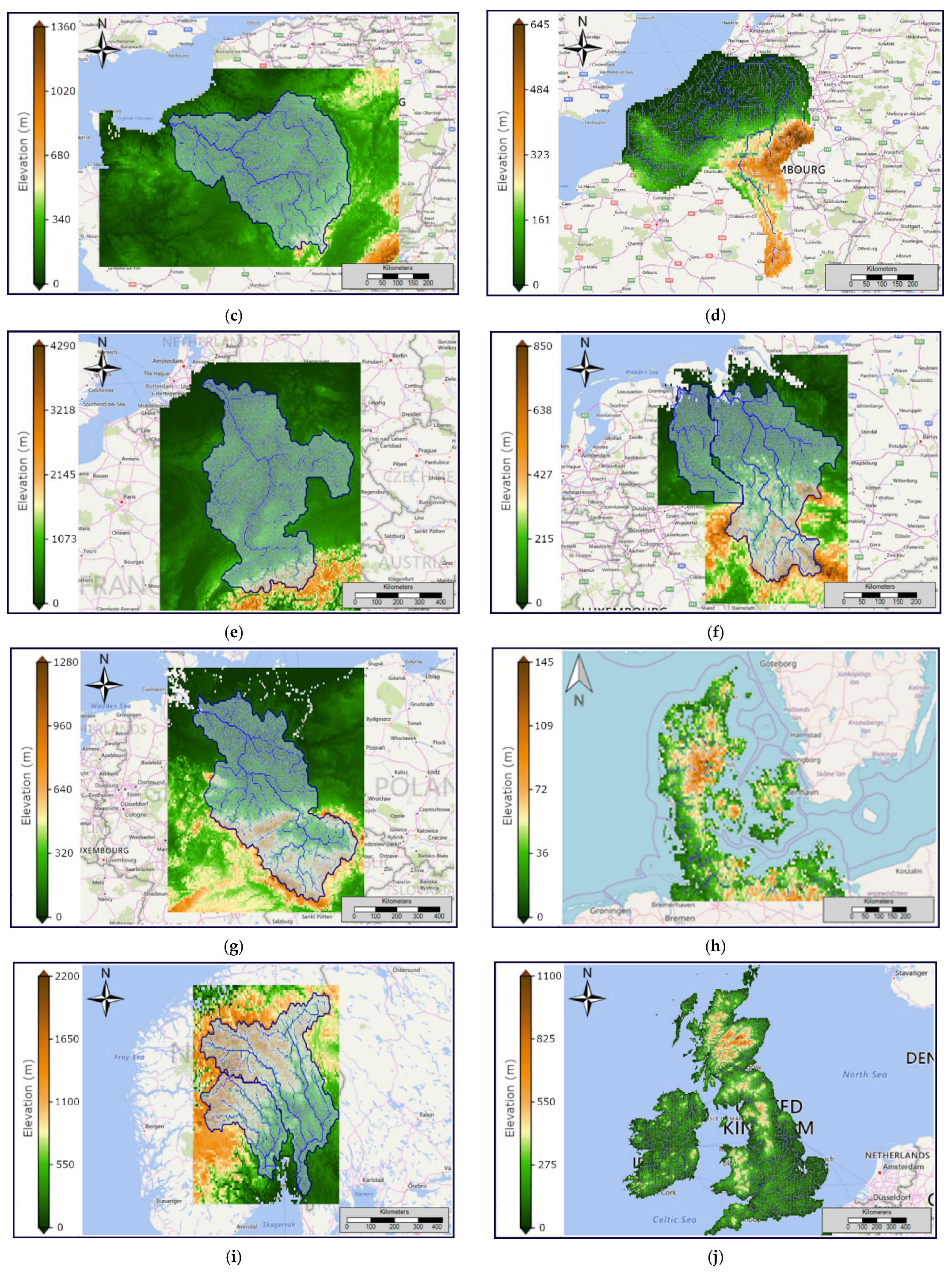
Each section of the water continuum, from the watershed to the open ocean, is reproduced with the different components of the MOHID Water Modelling System (http://www.mohid.com [9], accessed on 15 April 2022). The MOHID Water Modelling System is an open-source modular finite volume modelling system written in ANSI FORTRAN 95 with an object-oriented programming philosophy integrating several numerical programs accessible via the GitHub repository (https://github.com/Mohid-Water-Modelling-System/Mohid, accessed on 15 April 2022). MOHID Land and MOHID Water are the core numerical models.

2.1. Study Area

The largest rivers of the Iberian Peninsula other than the Ebro River discharge to the Atlantic coastal waters, draining almost two thirds of the territory along the way. In Portugal, river mouths are mostly situated in the northern part of the country, corresponding to the wettest region of the Iberian Peninsula with around 3000 mm of rain annually (Portuguese Water Atlas, https://sniamb.apambiente.pt/content/geo-visualizador, accessed on 15 April 2022).

Combined with the rain pattern, the concentration of river mouths in the Northwest Iberian coastal zone, such as the Douro, Minho, and Mondego rivers, provides the conditions required for the generation of a significant regional feature: the Western Iberia Buoyant Plume (WIBP; [10]). This is a year-round low-salinity water lens (S < 35.8), and it extends along the Northwest Iberian coast, influencing, among other things, ocean productivity (i.e., [11,12]) and larva and egg dispersal (i.e., [1,13,14,15,16]).

2.2. Watershed Modelling

The MOHID Land model is the hydrological model used to estimate river flow and water temperature for the study region. It is a physically based, spatially distributed, continuous, variable time-step model for inland water property cycles [17]. The model is based on finite volumes organized into a structured grid, rectangular in the horizontal plane, and z-level geometry in the vertical direction. It includes four compartments or media (atmosphere, porous, soil surface, and river network). Water moves through the mediums based on mass- and momentum-conservation equations. The atmosphere compartment provides varying space and time surface boundary conditions (precipitation, solar radiation, wind, etc.). The surface layer is described by a 2D horizontal grid, while the porous media consists of a 3D domain of variable-layer thickness that shares the horizontal grid with the surface layer. The river network is a 1D domain defined from the digital terrain model (DTM), with watershed reaches linking surface-cell centres. Fluxes are computed through the finite volumes’ sides, and state variables are computed at the cell centres to ensure transported properties are conserved. The model uses a dynamic time step that increases during dry periods and reduces as water fluxes increase (e.g., during rain events). The MOHID Land model can simulate single-catchment or multi-catchment domains. Although MOHID Land can be configured to simulate water properties such as oxygen, suspended sediment, and nutrient concentrations, in the LAMBDA project the simulations focused on obtaining river flows and water temperature.

The main objective of the watershed modelling simulations was to produce regional-scale water budgets covering the land boundary of the two CMEMS MFCs. For the LAMBDA project, the drainage basins draining the study area were divided into ten domains using regular grids with a horizontal resolution of 0.05° (Figure 1). Only the Loire (France) and the Severn (UK) rivers were simulated with higher resolutions due to developments during the Hazrunoff project (http://www.hazrunoff.eu/, accessed on 15 April 2022). In general, hydrologic models with a horizontal scale of 1–9 km resolution can obtain similar results and perform well for storm events [18]. The watershed and land-use grids were populated with the EU 30 m Digital Elevation Model (DEM) and Corine Land Cover 2012 obtained from the Copernicus Land Monitoring Service (https://land.copernicus.eu/, accessed on 15 April 2022), respectively. 3D soil hydraulic properties were obtained from Tóth et al. [19], while channel cross-sections were defined with the database from Andreadis et al. [20]. Each domain was simulated for the 2008–2019 period with meteorological conditions calculated with the ERA5 reanalysis product (horizontal resolution 31 km) from the Copernicus Climate Change Service (https://climate.copernicus.eu/, accessed on 15 April 2022).

2.3. Estuarine Modelling

Since regional ocean models commonly impose direct river discharges into coarse grids with horizontal resolutions of several kilometres, an estuarine proxy was developed to include the tidal signal complexity, thus providing more realistic readings of salinity concentration and of discharged volumes reaching the coastal area. This proxy was adapted from a more complex approach where full scale estuarine models were used to estimate transport fluxes and related water properties [7].

A simple and scalable MOHID Water application was designed to represent estuaries schematically and to export the methodology where a full-scale estuary model is not available. The advantages of this type of application include low computing costs and the capacity to combine realistic open ocean and land boundary conditions with local tides. The proxy can calculate a realistic tidal mixing, considering each estuary’s tidal prism, and different tidal cycles such as spring-neap and ebb-flow periods. Each proxy calculates cross-section water velocity that can later serve to impose momentum in the ocean model. Moreover, using a full numerical model to simulate in a simple grid, instead of tidal mixing empirical equations, allows for a future increase in complexity, i.e., adding atmospheric boundary conditions, biogeochemical modelling, etc.

The LAMBDA estuarine model proxy consists of a regular domain of 12 × 3 cells where the estuary is represented by 10 grid cells aligned in any cardinal direction plus a cell for the ocean open boundary conditions and the land boundary (Figure 2). Configuring each estuarine proxy domain requires some basic estuary geometry properties:

• Estuary depth: maximum, average, and minimum depth to populate the bathymetry grid cells;
• Estuary length: to configure the along-estuary grid cell size;
• Total area of the estuary: to estimate across-estuary cell size.
• Estuary mouth location: to define the grid origin and force of local tidal components;
• Estuary mouth orientation: to define the momentum velocity component (u or v) and its orientation;
• Ocean water properties: to force the open ocean boundary conditions.

At the open ocean boundary, the model generates water levels, using FES2014 tidal constituents, and receives ocean properties such as surface salinity and water temperature. Each estuarine proxy simulates its corresponding tides, supported by its georeferenced location, and using the FES2014 global tidal model [21]. Ocean-water properties at the open boundary can be defined as constant or time-varying with either timeseries or more complex 2D/3D fields from ocean global or regional models. In the innermost cell, river flow, temperature, and zero salinity is imposed.

Each estuarine proxy produces timeseries of flow, velocity (u or v according to estuary mouth orientation), and water properties estimated at its outer estuarine cell. Water velocity serves to impose momentum on the estuarine plume in the regional ocean model. In contrast with river discharges, modelled estuarine flows have positive and negative values according to the tidal phase (ebb and flood). The receiving model should be capable of handling negative discharges to fully include this property as a land boundary condition. The proxy outputs are independent of the downstream ocean model and for this reason can be applied to any regional or global ocean model.

To evaluate the performance of the estuarine proxy, simulations using this method were applied to the main six estuaries in western Iberia (from South to North): Guadalquivir, Sado, Tagus, Mondego, Douro, and Minho (Figure 3). Fluxes, temperature, salinity, and velocity timeseries were obtained for the period of May 2017–December 2018. The geomorphology information used to configure each of these estuary proxies is included in

Table 1. Proxy configuration for the main six estuaries in western Iberia ordered from South to North. The Tagus estuary is the only proxy configured with variable depth along its channel.

Estuary	Mouth Orientation	Cell Length (Degrees)	Cell Width (Degrees)	Ocean Depth (m)	Ocean Salinity	Estuary Depth (m)	Longitude Mouth (° W)	Latitude Mouth (° N)
Guadalquivir (ES)	West	0.11000	0.00475	20	36.2	10.0	6.440	36.785
Sado (PT)	West	0.08000	0.02000	10	36.0	8.0	8.930	38.470
Tagus (PT)	West	0.05000	0.06200	25	36.0	2.0–20.0	9.420	38.620
Mondego (PT)	West	0.00150	0.04500	6	36.0	2.0	8.880	40.143
Douro (PT)	West	0.02200	0.00272	8.2	36.0	8.2	8.700	41.140
Minho (PT-ES)	West	0.04000	0.00575	6	36.0	2.0	8.885	41.860

.

Two proxy scenarios were set according to observed and modelled land boundary conditions to assess human management impact on river flows. Observed river flows for the Douro, Guadalquivir, Mondego, and Tagus rivers were obtained from EMODnet physics near real time data (NRT). These were the only rivers with data available for the analysed period when the simulations were made. Water temperature was forced in all proxies with watershed modelling results, since this variable is rarely monitored continuously. Salinity was considered as freshwater with zero salinity in all land scenarios. At the open ocean boundary, each proxy received surface temperature and salinity values according to the locations of its mouth from a regional ocean model without land inputs, and the values are described in the next section.

2.4. Ocean Modelling

The LAMBDA boundary products were implemented as proof of concept (PoC) in an updated version Portuguese Coast Operational Modelling System (hereafter referred as PCOMS, [22,23]) that covers the western Iberia regional ocean. Simulations were made for the period of October 2017–December 2018 that includes the extreme rain event of late March 2018.

The PCOMS system is a 3D full baroclinic hydrodynamic and biogeochemical regional ocean operational model application that uses MOHID Water as its numerical core. It is composed of two nested domains: WestIberia (2D) and Portugal (3D) covering the Iberian Atlantic coast and its contiguous ocean populated with bathymetric information derived from the EMODnet Bathymetry portal (Figure 3; https://www.emodnet-bathymetry.eu/, accessed on 15 April 2022). The WestIberia domain covers the area limited by specific latitudes (33.48° N, 45.90° N) and longitudes (4.20° W, 13.50° W), resulting in a grid of 207 × 155 cells with a maximum depth around 5600 m. The Portugal domain covers the area comprised of specific latitudes (34.38° N, 45.00° N) and longitudes (5.10° W, 12.60° W), resulting in a grid of 177 × 125 cells and a maximum depth around 5300 m. Both domains use constant horizontal spatial resolution of 0.06°, resulting in 6.7 × 5.2 km cells. The Portugal domain is located at the centre of the WestIberia grid (Figure 3). Vertically, the Portugal domain uses a hybrid discretisation with near-surface, variable-thickness sigma layer with 7 levels, increasing from 1 m at the surface to 8.68 m of depth, above a layer with 43-z-levels increasing in thickness towards the bottom; this domain is based on the Mercator-Océan PSY2V4 vertical geometry [23].

Tides in the current configuration are also forced with FES2014 harmonic components along the WestIberia domain boundary. The Portugal domain receives tides from the WestIberia domain and uses CMEMS Global Ocean 1/12° Physics Analysis and Forecast updated Daily product (hereafter referred as CMEMS-Global) as initial and boundary condition for water levels, currents, temperature, and salinity. CMEMS-Global fields are relaxed in the first 10 cells of the open boundary, while the inner area the model runs free, without assimilation; these parameters rest on the assumption that the open ocean boundary condition does not affect the river-influenced areas. At the atmospheric boundary, the Portugal domain was forced by hourly results from a MM5 model application (Meteorological Model 5; [24]) based on two nested grids with a horizontal resolution of 27 and 9 km, respectively, implemented by the IST meteorological group (http://meteo.tecnico.ulisboa.pt/ [25], accessed on 15 April 2022).

3. Modelling Results and Validation

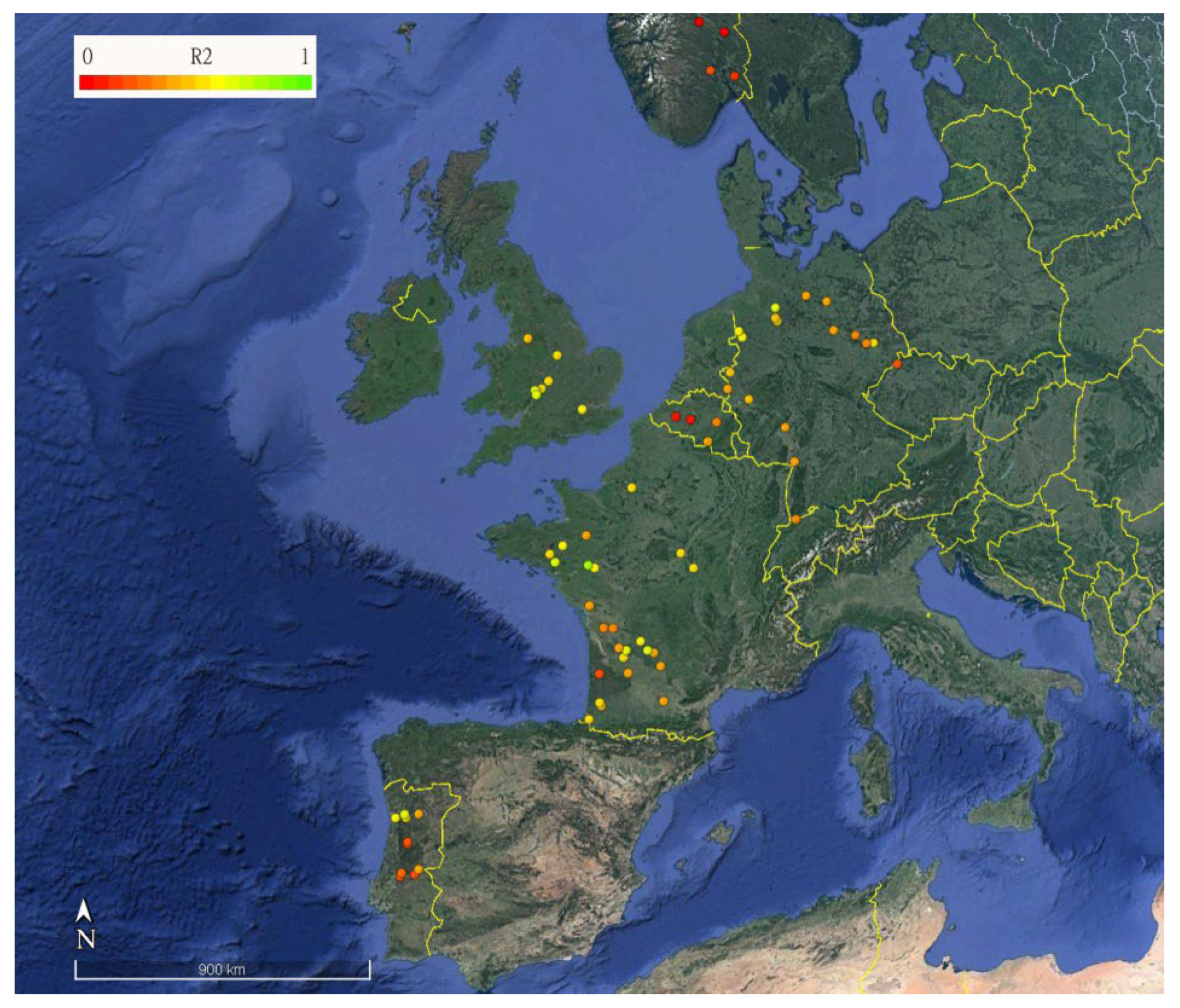
3.1. Watershed Modelling

Each modelling domain was independently calibrated, which resulted in flow and temperature timeseries for the main 54 rivers discharging into the European Atlantic Ocean and the North Sea for the period of 2008–2019. To achieve a more comprehensive water budget entering the coastal areas, 70 extra discharges for Western Iberia and 364 extra discharges for the Ireland and UK region were obtained from the domains. However, these extra rivers could not be fully validated, since resolution may be too coarse to accurately reproduce out-river flowrates.

Observed data for each river was collected from several data sources including EMODnet physics NRT river database (https://portal.emodnet-physics.eu/, accessed on 15 April 2022) for recent data and the Global Runoff Data Base (GRDB; https://www.bafg.de/GRDC/EN/01_GRDC/13_dtbse/database_node.html, accessed on 15 April 2022) for historical data. Nevertheless, the lack of available observations for some catchments or presented incomplete datasets for the simulation period hampered efforts to validate and calibrate some domains. Moreover, the available hydrologic stations are in some cases located far from the coastal area, so that validation was only possible for the upper part of the catchment. Figure 4 shows the geographic distribution of the coefficient of determination between observed and modelled data for the stations used for validation in this study.

A well-calibrated and -configured watershed model will face difficulties in attempting to accurately simulate river runoff, since river flow is highly controlled by reservoirs managed by human behaviour. Watershed numerical models calculate natural river flow, and as such, their results tend to be closer to the observed values when the degree of human intervention is low [17].

To illustrate the results, the analysis of two large rivers in western Iberia, the Douro and Tagus rivers, are presented. The Douro and Tagus river mouths are the longest rivers discharging in the Atlantic Ocean, at 897 and 1007 km long respectively. They receive waters from the largest drainage areas in the Iberian Peninsula, with 98,400 and 80,000 km² for the Douro and Tagus respectively. The larger Douro catchment is located in the wettest region of the Iberian Peninsula and with a resultant average flow of ≈700 m³ s⁻¹, an average that is higher than the Tagus River, whose average flow is ≈440 m³ s⁻¹. The river mouths are separated by 275 km.

Another subject relevant to the watershed validation is the precision of river flow observations, especially since many hydrometric stations use rating curves (RC) to transform water levels into river flow. This method may introduce some errors in the context of extreme events, since RC must be extrapolated outside of the observed range [26]. Such is the case for the Almourol station in the Tagus River where flow is calculated from water levels with a rating curve. On the other hand, the Douro River monitoring station closest to the coastal area (Albufeira da Crestuma) is a hydroelectric power plant, which enables more precise observation. In both rivers, the numerical model reproduces the main flow peaks in the period timeseries; however, it presents higher average flow and lower extreme peaks (Figure 5). This excess of freshwater may be caused by human management, errors, or uncertainties in the meteorological and watershed model and observations that translate into a low coefficient of determination of around 0.6 and 0.3 for the Douro and Tagus rivers, respectively.

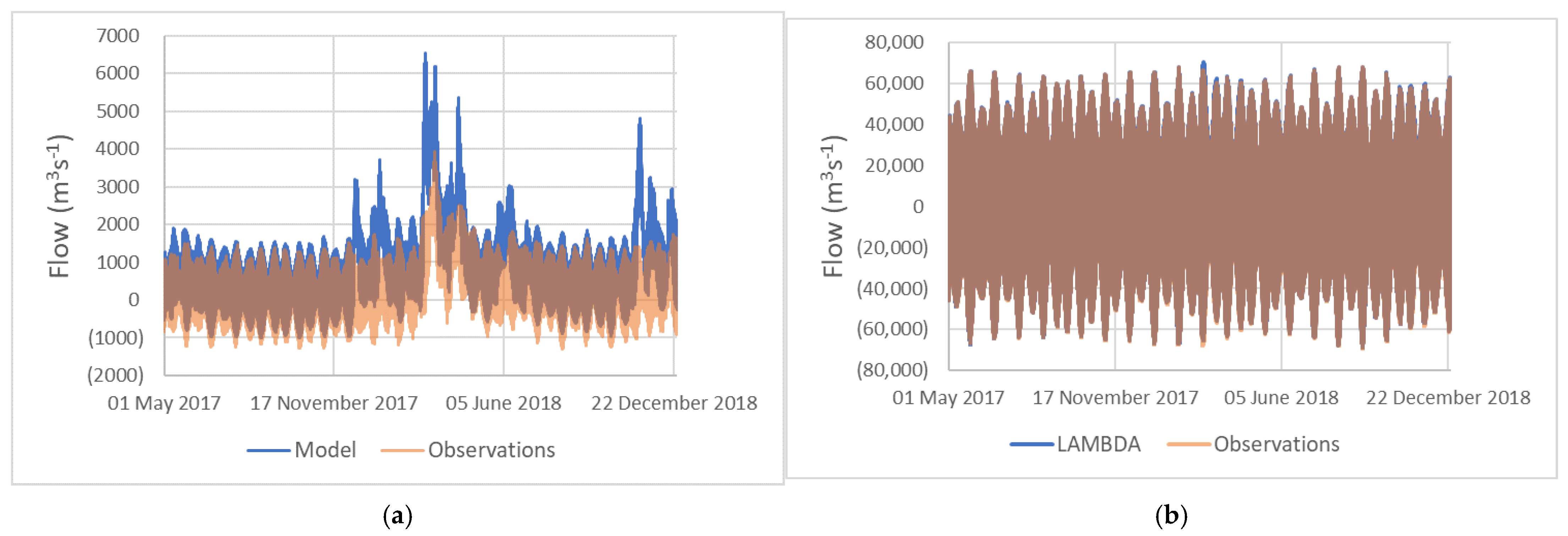
3.2. Estuary Modelling

To evaluate the differences resulting from using observed versus modelled river flow in the coastal area, the estuarine proxies defined for the Douro and the Tagus rivers were forced with both datasets for the period of May 2017–December 2018. These estuaries present large geomorphological differences (Table 1) relative to each other that affects their tidal prism size and substantially influences water volume and other properties reaching the open ocean (Figure 6). Mean maximum instant flow is around 1–1.5·10³ m³ s⁻¹ and 40–70·10³ m³ s⁻¹ for the Douro and Tagus estuaries, respectively. These values are similar to those found by Campuzano et al. [7] who used full-scale estuarine models. Larger volume fluxes do not imply larger momentum at the estuarine mouth. For example, the Douro estuary presents slightly larger instant velocities than the Tagus estuary that has larger estuarine flows (

Table 2. Basic statistics for the outputs from the Tagus and Douro proxies when forced with observed flows (Obs.) and when forced with watershed models (Model). * Values were calculated with the absolute values.

		Tagus			Douro
		Max.	Min.	Avg.	Max.	Min.	Avg.
Observations	Flow (m3 s−1)	68,231.84	−68,663.64	29,264.75 *	3936.56	−1307.51	654.20 *
	Velocity (m s−1)	0.45	−0.46	0.19 *	0.42	−1.30	0.21 *
	Temperature (°C)	20.08	12.85	16.61	26.80	1.63	15.12
	Salinity	35.62	26.47	33.84	34.93	0.017	12.50
Model	Flow (m3 s−1)	70,483.38	−68,614.38	29,255.41 *	6535.13	−1017.03	1034.52 *
	Velocity (m s−1)	0.45	−0.47	0.19 *	0.33	−2.21	0.33 *
	Temperature (°C)	20.51	9.68	16.53	27.23	1.22	14.81
	Salinity	35.15	5.05	30.71	30.12	0.01	3.39

). During extreme events, as in March 2018, Tagus flow and velocity were barely impacted by the river discharge while the Douro estuary was highly affected by this type of event, with flows and velocities substantially affecting the plume momentum, shape, and extension.

The differing geomorphologies are also important for the water properties reaching the coastal area. When forced with the observed values of the river flow, the average salinity at the mouth of the Tagus estuary is around 33 salinity units, while in the Douro the average salinity is only 12.5 salinity units. In terms of the S-value range, the Douro has a greater variability than the Tagus estuary. During extreme conditions, freshwater conditions can almost be reached in the Douro mouth, as was also observed with the full-scale estuary model [7]. The Douro estuary temperature range is also widely impacted by the river’s seasonal temperature evolution.

Proxies forced with LAMBDA watershed modelling results lead to fresher water for both estuaries. Nevertheless, salinity trends are well represented for both estuaries. The Douro estuary proxy, due to its smaller size, is more sensitive to differences in the imposed river flow.

3.3. Ocean Modelling

Six land boundary configurations were defined to evaluate the impact of river influence on the ocean waters of western Iberia. Meteorological and open ocean boundary conditions were the same for all the scenarios. The scenarios are:

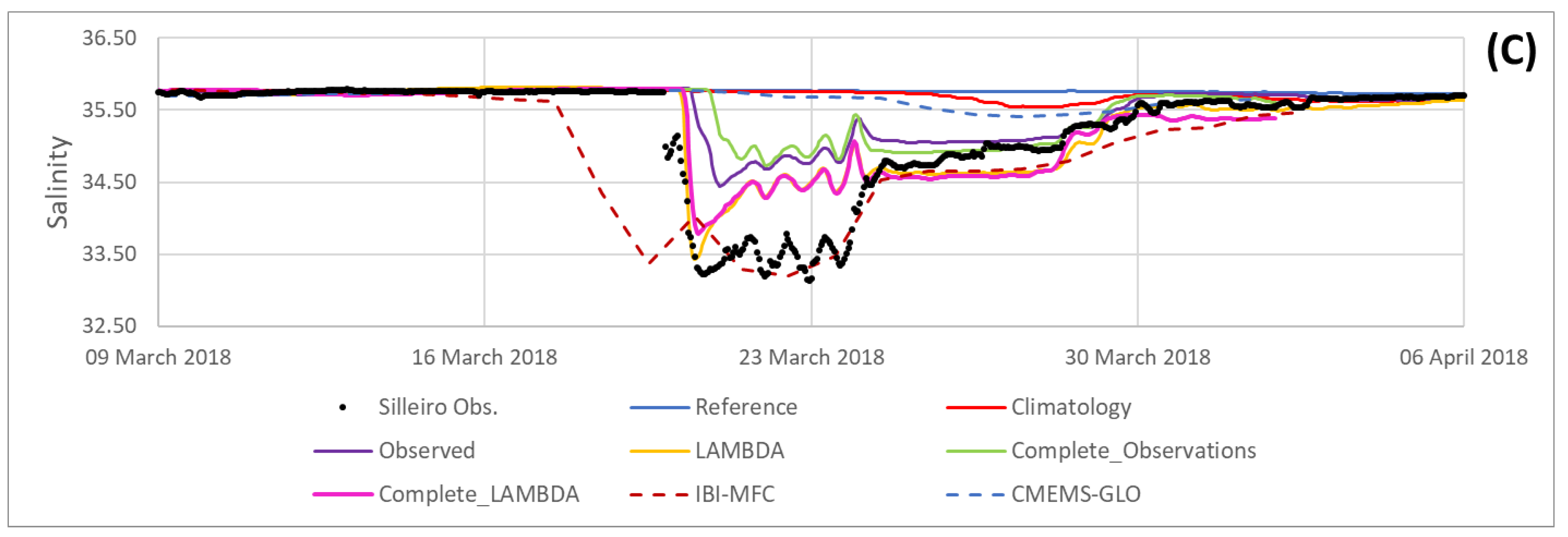
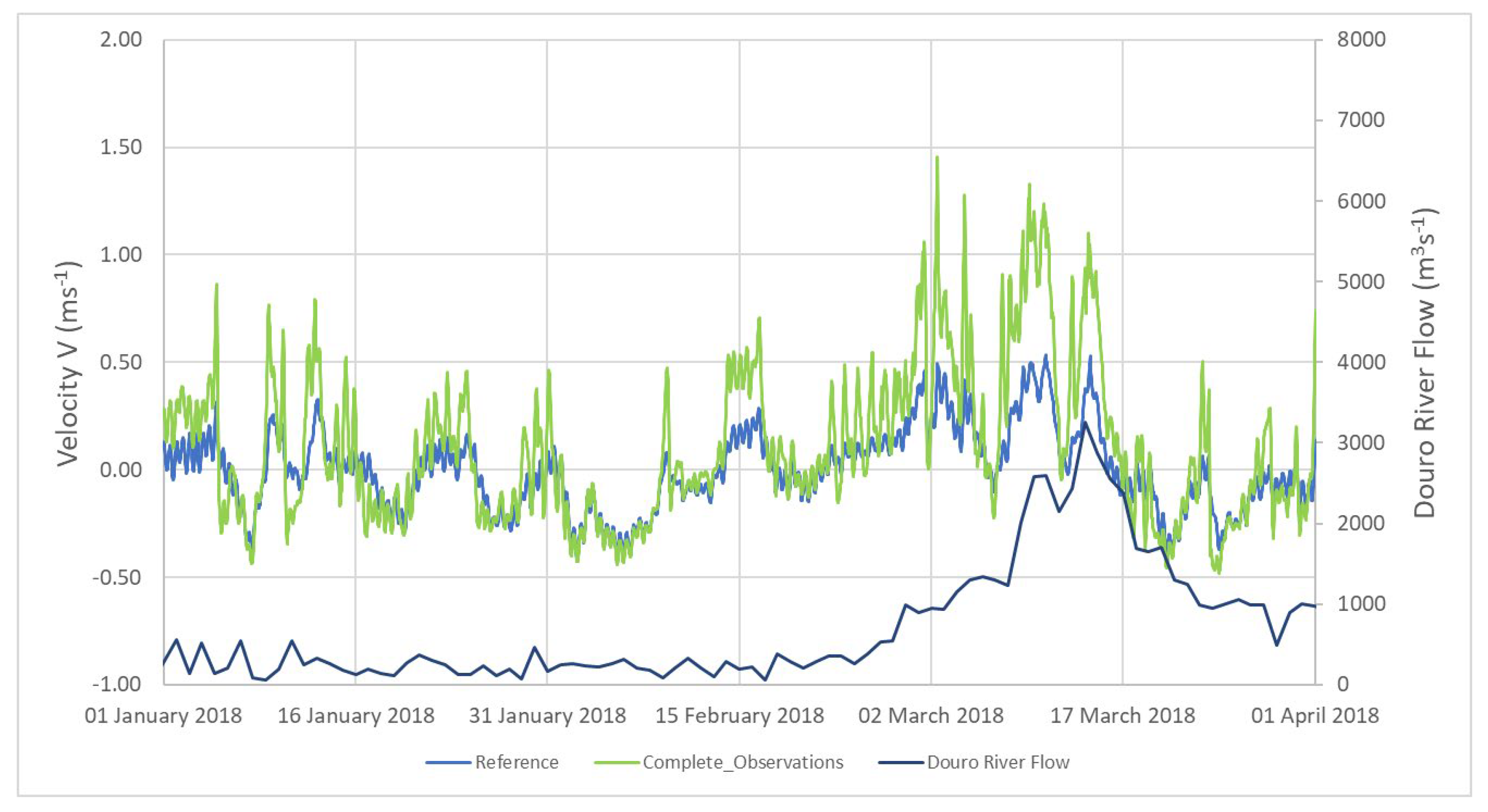
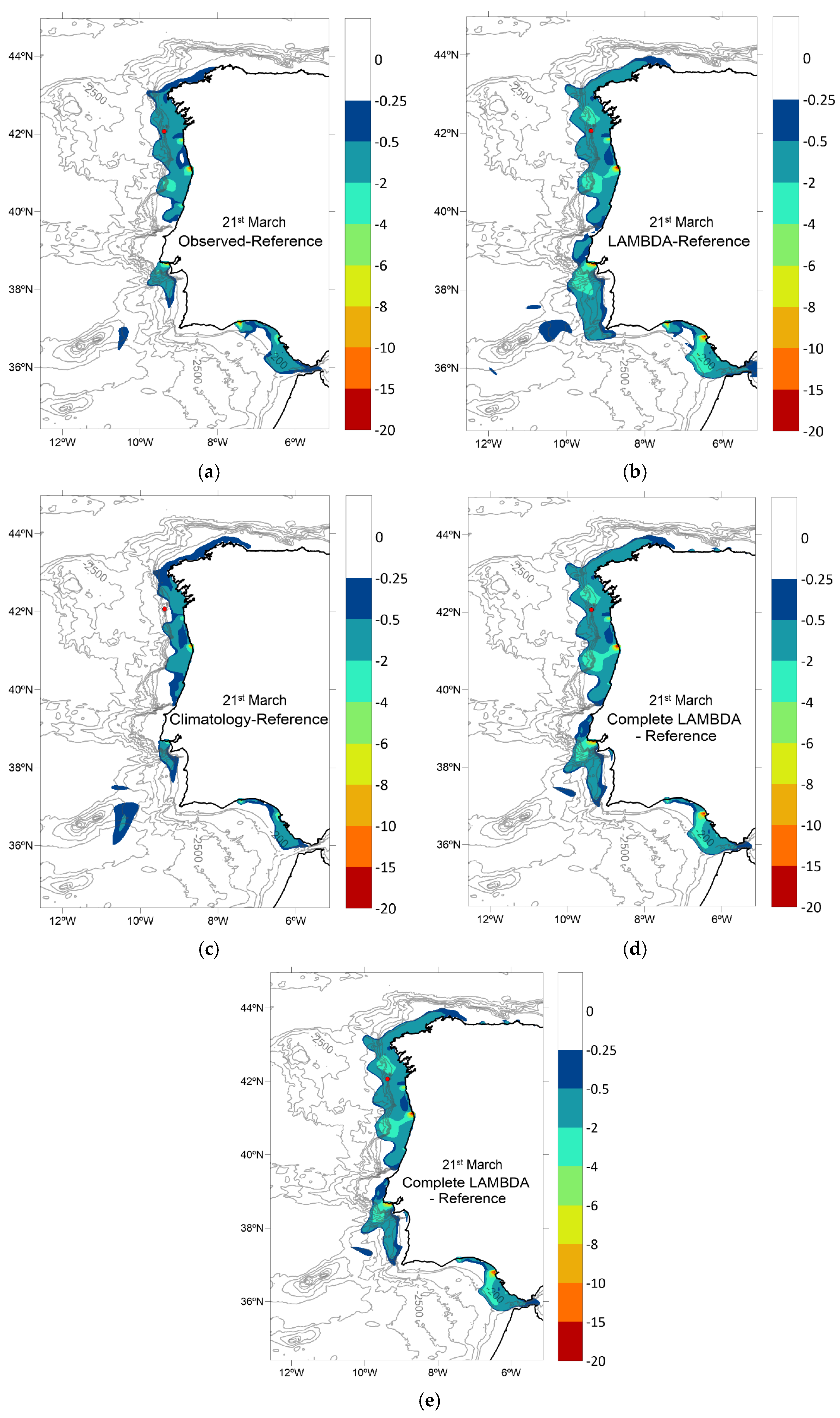
• Reference: model running continuously, since 2017, without any land input thus considered the baseline to evaluate the rivers’ impact;
• Climatology: direct surface river discharge of climatological values for flow and temperature with only rivers included in IBI-MFC (Douro, Guadiana, Guadalquivir, Minho, Mondego, Tagus);
• LAMBDA: the same rivers and methods as Climatology scenario with river flow and temperature obtained from the LAMBDA Watershed product;
• Observed: the same rivers and methods as Climatology but observed flow for Douro, Guadalquivir, Mondego and Tagus. River temperature from the LAMBDA watershed product;
• Complete Observations: six main estuaries (Minho, Douro, Mondego, Tagus, Sado and Guadalquivir) corrected by estuarine proxy. Also, an additional 45 rivers (Figure 3) discharged directly with the LAMBDA modelled flow and temperature with constant salinity S 25.
• Complete LAMBDA: the same as the Complete Observations scenario with all river information obtained from the LAMBDA watershed model results.

3.3.1. PCOMS Validation

The PCOMS model application was forced with each land boundary condition scenario. The results were analysed in order to better understand the response of the numerical model’s different land forcings. The analysis focused on the first quarter of 2018, corresponding to a wet season period, and includes an extreme rain event in late March. The obtained modelling results were compared with in-situ operational observations, remote sensing products, and state-of-the-art regional and global operational ocean models for the same study area.

Results from each land boundary scenario were compared with salinity and temperature values recorded by the Silleiro buoy. This buoy, belonging to the Puertos del Estado monitoring network, is located 50 km offshore of northwestern Iberia (coordinates: 42.119° N, 9.440° W; Figure 3). When high river discharges coincide with upwelling prevailing wind conditions, northern winds for this coastal stretch, the WIBP signature can be detected in the salinity and temperature records [23].

Observed surface salinity records remained almost constant in January 2018 at the Silleiro buoy. However, direct discharge scenarios such as Observed and LAMBDA exhibited a salinity decrease around 8 January. This was not reproduced by the scenarios using the estuarine proxy: Complete Observations and Complete LAMBDA (Figure 7). The complete scenarios receive land boundary salinity values that have been previously mixed in the estuarine proxy, while direct discharge scenarios are forced using zero salinity conditions (Figure 6). Moreover, estuarine fluxes have positive and negative fluxes while the direct discharge scenarios are releasing continuously lower salinity discharges.

To compare the present methodology results with state-of-the-art operational models, timeseries from CMEMS-Global and IBI-MFC were added to this work scenarios (Figure 7). The IBI-MFC is the regional ocean model of the European Commission Copernicus Programme based on a NEMO model application run at a horizontal resolution of 0.028° (≈2.40 km). This model implementation, operated by Puertos del Estado and Mercator-Océan, includes high frequency processes (i.e., tidal forcing, surges and high frequency atmospheric forcing, freshwater river discharge, etc.). CMEMS models use land boundary conditions drawn from monthly river climatology, conditions that are directly discharged at the surface layer.

In late February, another salinity decrease was observed but overestimated, mainly in direct discharge scenarios. The Climatology scenario presents lower salinity than the Observed scenario, due to the Douro River climatology flow for February; 1140 m³ s⁻¹ is much larger than observe values for February 2018, which only reached 264 m³ s⁻¹.

During the extreme rain event in late March, salinity values decreased by more than 2.5 salinity units and its signal lasted more than 10 days with its main peak on 22 March. The LAMBDA scenario is the direct discharge scenario that best represented this event, as the excess of freshwater estimated by the watershed model for the Douro River, two times more than observed, compensates the lack of other river sources. From this result, we concluded that it is essential to have the right freshwater budget draining in the study area to represent accurately this type of event. In the LAMBDA scenario, only two rivers, Minho and Douro, are discharging close to the buoy area, while in reality there are many other smaller watersheds that can contribute to generate this large salinity signature. CMEMS-Global results clearly underestimate the largest freshwater event, while IBI-MFC obtains good results for the extreme event. It does however overestimates other earlier events.

When the estuarine proxy is used, additional river contributions are needed to achieve similar salinity changes. In the scenarios using the proxy, Complete Observations and Complete LAMBDA, a constant salinity of 25 salinity units for the other rivers was considered as a compromise to the average salinity from different types of estuaries (Table 2). Nevertheless, this approach still seems very conservative, and salinity did not decrease as observed. It is probable that estuaries in the area have a geomorphology similar to the Douro estuary and may contribute to lower salinity values. Further analyses and experiments are needed to evaluate how minor rivers could be included and parameterised. A possible solution to explore in future works is to implement estuarine proxies for the smaller rivers.

Regarding sea surface temperature (SST), modelling results tend to represent quite accurately the main trends during the analysed period (Figure 8). As with salinity, January temperature drops a great deal in the direct discharge scenarios (Observed, LAMBDA and Climatology). However, during the extreme event, the scenarios using LAMBDA-simulated temperature were the only scenarios capable of reproducing the temperature drop. The statistical analysis of the surface temperature at this location (

Table 3. Surface salinity and temperature coefficient of determination (R²), Root Mean Square Error (RMSE) and Mean Absolute Error (MAE) between the observations of Silleiro buoy and each PCOMS configuration using LAMBDA boundary conditions scenario for the period of 1 January–4 January 2018. The Complete scenarios are the only ones using the proxy.

	Property	Reference	Climatology	Observed	LAMBDA	Complete Observations	Complete LAMBDA
R2	Salinity	0.07	0.00	0.65	0.72	0.61	0.78
	Temperature	0.71	0.70	0.80	0.79	0.81	0.80
RMSE	Salinity	0.52	0.52	0.32	0.26	0.35	0.23
	Temperature	0.36	0.42	0.36	0.41	0.36	0.40
MAE	Salinity	0.27	0.27	0.10	0.07	0.12	0.06
	Temperature	0.13	0.18	0.13	0.17	0.13	0.16

) showed that any scenario including rivers improved the estimation of SST with the only exception being the Climatology scenario.

To evaluate the possible impact of river discharges on the coastal hydrodynamics, the meridional velocity in the vicinity of A Guarda (Figure 3), located in the Minho estuary mouth and around 80 km north of the Douro mouth, was obtained for the Reference scenario, with no river inputs, and the Complete Observations scenario. The Complete Observations scenario achieved a meridional velocity up to three times that of the Reference scenario. Figure 9 shows that during the highest peak of river discharges (i.e., Douro River reached values around 3200 m³ s⁻¹), the Reference scenario presented values around 0.5 m s⁻¹ while more realistic land boundary scenarios can reach maximum values around 1.5 m s⁻¹.

Earth Observations (EO) products can play an important role for model validation. They provide a spatial and temporal coverage that yields complete and verified information obtained by the numerical models. The remote sensing product chosen to evaluate the sea-surface temperature (SST) of the PCOMS modelling results is the Multi-scale Ultra-high Resolution (MUR). The MUR version 4.1 used in this study (http://dx.doi.org/10.5067/GHGMR-4FJ04, accessed on 15 April 2022) provides daily SST estimates on a global 0.01° × 0.01° grid and features the 1-km resolution MODIS retrievals, which are fused with AVHRR GAC, microwave, and in-situ SST data by applying internal correction for relative biases among the data sets [27]. In Figure 10, SST- and PCOMS-model results forced with LAMBDA Complete Observations scenario display similar structures and values for western Iberia during the extreme rain event peak. In the image, the colder temperature signature of the Douro, Tagus, and Guadalquivir rivers’ individual plumes as well as other smaller rivers can be easily identified.

Finally, modelling results were compared with Earth Observed (EO) salinity-derived products developed in the context of the LAMBDA project [28]. This new SMOS SSS global product was developed with the main goal of capturing the coastal processes. This L4 SMOS SSS product allows downscaling the salinity by using as a template the Sea Surface Temperature (SST) at 0.05° from OSTIA. EO and numerical modelling results for the extreme event of late March 2018 present similar spatial structures and intensities (Figure 11). Though using satellite-derived SSS still has many drawbacks, i.e., low horizontal resolution to capture some coastal variability, this comparison indicates a promising evolution of these kinds of products for data analysis and model validation for coastal areas.

3.3.2. Scenario Analysis

Each of the Ocean scenarios was evaluated in terms of WIBP low salinity extension for two periods: (i) considering average values for a typical wet month (February 2018; Figure 12) and during the peak of an extreme rain event (21 March 2018; Figure 13).

During February 2018 (Figure 12), the Climatology, LAMBDA, and Complete LAMBDA scenarios exhibited the greatest extension of the West Iberia Buoyant Plume (WIBP), while scenarios using river observations (Observed and Complete Observations) had their plumes more confined near the coastal area. The latter group also exhibited a relatively reduced Tagus estuary plume (latitude 38.6). The scenarios using the estuarine proxy (Complete scenarios) reduced the extension of the plume relative to the direct discharges’ scenarios, even when these included an additional 45 rivers with a constant value of 25 salinity units.

A similar pattern of results is observed during the extreme rain event for each modelling scenario. Figure 13 represents the mean SSS for the 21 March 2018, a day after the salinity minimum was registered at the Silleiro buoy. Though the Climatology scenario appears to have a similar spatial distribution during the event, it does not reach the minimum temperature and salinity values displayed in Figure 7. In addition, the Tagus estuary plume appears to be overestimated by the Climatology and LAMBDA scenarios when compared to the Observed scenario. The effect of the proxy in the Tagus estuary is clearly noticed in the Complete Observed scenarios where its impact is reduced.

4. Discussion

By improving the calculation of the freshwater quantity and associated properties reaching the coastal area, managers and scientists would be able to better reproduce the thermal and salinity fronts affecting coastal hydrodynamics and associated ecological processes. The proposed methodology for integrating the water cycle from rainwater runoff to the open ocean with numerical models was demonstrated for western Iberia by simulating the extension of the WIBP during a wet season and an extreme rain event.

The approach taken enables the continuous improvement of the solution through updates/upgrades to any upstream component such as the watershed results or through the use of a better characterisation of the estuarine proxy. The application of this methodology provides more realistic land boundary conditions than river climatology direct discharges, while also having the capacity to describe inter-annual variability between dry and wet years and effects due to extreme rain or drought events. The developed methodology is generic and could be set for any region with open-access data and open-source models.

Enhanced land boundary conditions including water properties such as temperature and salinity can provide a more realistic circulation and thermohaline fields in the coastal area. The included land boundary conditions can grow in complexity from plainly watershed modelling results that are implemented as direct discharges to fully 3D biogeochemical estuarine fluxes (positive and negative) imposed with momentum.

The main advantage of watershed modelling is to complete the hydrometric monitoring networks, providing gapless river-flow data and non-monitored variables while covering areas with monitored data. Additionally, watershed numerical modelling enables the forecasting of river flow and water properties, thereby allowing a more efficient management of the modelled systems. However, calibration and validation of many watersheds became challenging when large water reservoirs or intense human management modify their natural flow. The use of 5 km horizontal-resolution domains enabled the coverage of a large simulation area, as well as a decrease in the simulation time required, and these domains can adequately represent the channel flow behaviour of larger rivers. However, smaller rivers may not be accurately simulated under these conditions. Generally, better results are obtained from higher resolution grids and single-watershed domains, since calibration is easier to execute.

From an operational point of view, the objective is to generate a land boundary product with the best available information. For this reason, observed data can be combined with modelling results, such as river properties. In any case, the watershed-model approach has shown the ability to produce a more realistic land boundary condition than methods involving the use of river climatologies, but further development is needed for this component of the system.

The estuarine proxy has been a versatile tool that allows researchers to estimate in a simple way estuarine mixing and contributions to the open ocean. The proxy affords the inclusion of estuary time and spatial scales, due to the tides and the rivers’ flow combination, in coarse regional ocean models. Its low computational cost would enable the easy construction of two-way coupled systems. Another advantage is that land boundary conditions are independent of the receiving model domain, and thus the same flow/fluxes can be used by several regional ocean models. The estuarine proxy can be regarded as a useful tool when full estuarine models do not exist.

5. Conclusions and Future Approach

Monitoring networks along the estuarine continuum from river catchment to the open ocean should be encouraged for evaluating the transfer of properties and momentum at the land-ocean interface. While open ocean network is relatively well established, operational estuarine monitoring is far from consolidated. In general, hydrometric networks should be further developed to meet the requirements of coastal region stakeholders. Numerical models can support the design of the monitoring networks, and they can provide a more comprehensive view by spatially and temporally completing the observed data. In addition, numerical models can provide non-observed variables and forecasts. Model results also permit the calculation of complex indicators such as tidal prims and the area of influence of the estuarine waters, as well as the accurate estimation of estuarine fluxes that would serve as boundary conditions for ocean regional models. The synergies between these two can be observed, and the modelled data pave the way for a more holistic view of the water continuum.

Since salinity remote sensing is starting to take its first steps in coastal areas and since in-situ monitoring has a low frequency, numerical modelling is currently the only tool able to represent and estimate the temporal and spatial scale of the WIBP and other estuarine plumes. Taking into consideration the numerical modelling limitations and assumptions, the salinity modelling results provided by the methodology described here significantly improves salinity fields and helps delimit the region of freshwater influence and salinity fronts.

Future work must include improving the incorporation of human-water management in watershed modelling in order to obtain more accurate forecasts. A possible next step in the research is to use artificial intelligence and machine learning techniques. In fact, combining machine learning and physical-based models is becoming popular in the design of predictive systems [29,30]. Including the human component is especially relevant in southern Europe where water retention is a more common practice.

In addition, efforts to identify and make available more river data are crucial for watershed-model calibration and validation. As the results show, to achieve good sea surface salinity fields in regional models, it is not enough to include only the major rivers, but a comprehensive freshwater budget is also required.

References

1. Garvine, R.W.; Whitney, M.M. An estuarine box model of freshwater delivery to the coastal ocean for use in climate models. J. Mar. Res. 2006, 64, 173–194. [Google Scholar] [CrossRef]
2. Santos, A.M.P.; Chícharo, A.; Dos Santos, A.; Moita, T.; Oliveira, P.B.; Peliz, Á.; Ré, P. Physical—Biological interactions in the life history of small pelagic fish in the Western Iberia Upwelling Ecosystem. Prog. Oceanogr. 2007, 74, 192–209. [Google Scholar] [CrossRef]
3. Banas, N.S.; MacCready, P.; Hickey, B.M. The columbia river plume as cross-shelf exporter and along-coast barrier. Cont. Shelf Res. 2009, 29, 292–301. [Google Scholar] [CrossRef]
4. Mishra, A.K.; Coulibaly, P. Developments in hydrometric network design: A review. Rev. Geophys. 2009, 47, RG2001. [Google Scholar] [CrossRef]
5. Campuzano, F.; Brito, D.; Juliano, M.; Fernandes, R.; de Pablo, H.; Neves, R. Coupling watersheds, estuaries and regional ocean through numerical modelling for Western Iberia: A novel methodology. Ocean. Dyn. 2016, 66, 1745–1756. [Google Scholar] [CrossRef]
6. Schiller, R.V.; Kourafalou, V.H. Modeling river plume dynamics with the Hybrid Coordinate Ocean Model. Ocean. Model. 2010, 33, 101–117. [Google Scholar] [CrossRef]
7. Campuzano, F.J.; Juliano, M.; Sobrinho, J.; de Pablo, H.; Brito, D.; Fernandes, R.; Neves, R. Coupling Watersheds, Estuaries and Regional Oceanography through Numerical Modelling in the Western Iberia: Thermohaline Flux Variability at the Ocean-Estuary Interface; Froneman, E.W., Ed.; IntechOpen: London, UK, 2018; pp. 1–17. [Google Scholar] [CrossRef] [Green Version]
8. Sotillo, M.G.; Campuzano, F.; Guihou, K.; Lorente, P.; Olmedo, E.; Matulka, A.; Santos, F.; Amo-Baladrón, M.A.; Novellino, A. River freshwater contribution in operational ocean models along the European Atlantic Façade: Impact of a new river discharge forcing data on the CMEMS IBI Regional Model solution. J. Mar. Sci. Eng. 2021, 9, 401. [Google Scholar] [CrossRef]
9. Neves, R. The MOHID concept. In Ocean Modelling for Coastal Management—Case Studies with MOHID; Mateus, M., Neves, R., Eds.; IST Press: Lisbon, Portugal, 2013; pp. 1–11. [Google Scholar]
10. Peliz, Á.; Rosa, T.L.; Santos, A.M.P.; Pissarra, J.L. Fronts, jets, and counter-flows in the Western Iberian upwelling system. J. Mar. Syst. 2002, 35, 61–77. [Google Scholar] [CrossRef]
11. Ribeiro, A.C.; Peliz, Á.; Santos, A.M.P. A study of the response of chlorophyll-a biomass to a winter upwelling event off Western Iberia using SeaWiFS and in situ data. J. Mar. Syst. 2005, 53, 87–107. [Google Scholar] [CrossRef]
12. Picado, A.; Dias, J.M.; Fortunato, A. Tidal changes in estuarine systems induced by local geomorphologic modifications. Cont. Shelf Res. 2010, 30, 1854–1864. [Google Scholar] [CrossRef] [Green Version]
13. Santos, A.M.P.; Peliz, Á.; Dubert, J.; Oliveira, P.B.; Angélico, M.M.; Ré, P. Impact of a winter upwelling event on the distribution and transport of sardine (Sardina pilchardus) eggs and larvae off western Iberia: A retention mechanism. Cont. Shelf Res. 2004, 24, 149–165. [Google Scholar] [CrossRef]
14. Santos, A.M.P.; Ré, P.; dos Santos, A.; Peliz, Á. Vertical distribution of the European sardine (Sardina pilchardus) larvae and its implications for their survival. J. Plankton Res. 2006, 28, 523–532. [Google Scholar] [CrossRef] [Green Version]
15. Peliz, A.; Marchesiello, P.; Dubert, J.; Marta-Almeida, M.; Roy, C.; Queiroga, H. A study of crab larvae dispersal on the Western Iberian Shelf: Physical processes. J. Mar. Syst. 2007, 68, 215–236. [Google Scholar] [CrossRef]
16. Queiroga, H.; Cruz, T.; dos Santos, A.; Dubert, J.; González-Gordillo, J.I.; Paula, J.; Peliz, Á.; Santos, A.M.P. Oceanographic and behavioural processes affecting invertebrate larval dispersal and supply in the western Iberia upwelling ecosystem. Prog. Oceanogr. 2007, 74, 174–191. [Google Scholar] [CrossRef]
17. Brito, D.; Campuzano, F.J.; Sobrinho, J.; Fernandes, R.; Neves, R. Integrating operational watershed and coastal models for the Iberian Coast: Watershed model implementation—A first approach. Estuar. Coast. Shelf Sci. 2015, 167, 138–146. [Google Scholar] [CrossRef]
18. Tian, J.; Liu, J.; Wang, Y.; Wang, W.; Li, C.; Hu, C. A coupled atmospheric–hydrologic modeling system with variable grid sizes for rainfall—Runoff simulation in semi-humid and semi-arid watersheds: How does the coupling scale affects the results? Hydrol. Earth Syst. Sci. 2020, 24, 3933–3949. [Google Scholar] [CrossRef]
19. Tóth, B.; Weynants, M.; Pásztor, L.; Hengl, T. 3D soil hydraulic database of Europe at 250 m resolution. Ecohydrology 2016, 31, 2662–2666. [Google Scholar] [CrossRef] [Green Version]
20. Andreadis, K.A.; Schumann, G.J.-P.; Pavelsky, T. A simple global river bankfull width and depth database. Water Resour. Res. 2013, 49, 7164–7168. [Google Scholar] [CrossRef]
21. Carrère, L.; Lyard, F.; Cancet, M.; Guillot, A.; Picot, N. FES2014, a new tidal model—Validation results and perspectives for improvements. In Proceedings of the ESA Living Planet Conference, Prague, Czech Republic, 9–13 May 2016. [Google Scholar]
22. Mateus, M.; Riflet, G.; Chambel, P.; Fernandes, L.; Fernandes, R.; Juliano, M.; Campuzano, F.; de Pablo, H.; Neves, R. An operational model for the West Iberian coast: Products and services. Ocean. Sci. 2012, 8, 713–732. [Google Scholar] [CrossRef] [Green Version]
23. Campuzano, F. Coupling Watersheds, Estuaries and Regional Seas through Numerical Modelling for Western Iberia. Ph.D. Thesis, Instituto Superior Técnico, Universidade de Lisboa, Lisbon, Portugal, 2018. [Google Scholar]
24. Grell, G.A.; Dudhia, J.; Stauffer, D. A Description of the Fifth-Generation Penn State/NCAR Mesoscale Model (MM5); Technical Note No.NCAR/TN-398+STR; University Corporation for Atmospheric Research: Boulder, CO, USA, 1994. [Google Scholar] [CrossRef]
25. Trancoso, A.R. Operational Modelling as a Tool in Wind Power Forecast and Meteorological Warnings. Ph.D. Thesis, Instituto Superior Técnico, Universidade Técnica de Lisboa, Lisbon, Portugal, 2012. [Google Scholar]
26. Sikorska, A.E.; Scheidegger, A.; Banasik, K.; Rieckermann, J. Considering rating curve uncertainty in water level predictions. Hydrol. Earth Syst. Sci. 2013, 17, 4415–4427. [Google Scholar] [CrossRef] [Green Version]
27. Chin, T.M.; Vazquez-Cuervo, J.; Armstrong, E.M. A multi-scale high-resolution analysis of global sea surface temperature. Remote Sens. Environ. 2017, 200, 154–169. [Google Scholar] [CrossRef]
28. Olmedo, E.; González-Haro, C.; Hoareau, N.; Umbert, M.; González-Gambau, V.; Martínez, J.; Gabarró, C.; Turiel, A. Nine years of SMOS sea surface salinity global maps at the Barcelona Expert Center. Earth Syst. Sci. Data 2021, 13, 857–888. [Google Scholar] [CrossRef]
29. Yaseen, Z.M.; Sulaiman, S.O.; Deo, R.C.; Chaud, K.-W. An enhanced extreme learning machine model for river flow forecasting: State-of-the-art, practical applications in water resource engineering area and future research direction. J. Hydrol. 2019, 569, 387–408. [Google Scholar] [CrossRef]
30. Sarafanov, M.; Borisova, Y.; Maslyaev, M.; Revin, I.; Maximov, G.; Nikitin, N.O. Short-term river flood forecasting using composite models and automated machine learning: The case study of Lena river. Water 2021, 13, 3482. [Google Scholar] [CrossRef]
Figure 1. Topography and drainage network of the LAMBDA project watershed domains. The LAMBDA watershed domains are: (a) Western Iberian Peninsula domain; (b) Western France domain; (c) Seine River domain; (d) Somme, Scheldt, and Meuse rivers domain; (e) Rhine River domain; (f) Northwest Germany domain; (g) Elbe River domain; (h) Denmark domain; (i) Southern Norway domain; (j) United Kingdom and Ireland domain.
Jmse 10 00852 g001aJmse 10 00852 g001b
Figure 2. MOHID Water Estuarine schematic model design used for simulating an estuarine proxy. The domain consists of a 12 × 3 grid that receives land inputs (river flow, temperature and salinity) and ocean inputs from tides and regional ocean models (water level, currents, temperature, and salinity) to produce outputs at the estuarine mouth, outputs such as salinity, temperature, flow, and velocity.
Jmse 10 00852 g002
Figure 3. PCOMS regional ocean operational system domains and bathymetry. The full domain corresponds to the WestIberia 2D Domain where tide is imposed. The red box indicates the outer limit of the Portugal 3D Domain. Pink dots indicate the location of the six main estuaries in western Iberia. Red dots indicate the location of extra 45 rivers implemented with direct discharges. The locations of Silleiro and A Guarda monitoring stations are indicated by orange dots.
Jmse 10 00852 g003
Figure 4. Coefficient of determination (R2) between observed and modelled river flow for the stations with available data for the period 2008–2019.
Jmse 10 00852 g004
Figure 5. Observed (orange line) and modelled (blue line) river flow for the period 2014–2018 used for validation in (a) Douro River at Albufeira de Crestuma station; (b) Tagus River at Almourol station (Source for observed data: Portuguese Environmental Agency APA).
Jmse 10 00852 g005
Figure 6. Flow (a,b), zonal velocity (c,d), salinity (e,f) and temperature (g,h) obtained at the mouth of the estuary proxy forced with observed (Orange line) and modelled (Blue line) river flows in the Douro (left) and Tagus (right) estuaries for the period of May 2017–December 2018. Brown colours indicate overlapping values.
Jmse 10 00852 g006aJmse 10 00852 g006b
Figure 7. Sea surface salinity observed (black dots) and modelled at Silleiro buoy during the first quarter of 2018. PCOMS modelling scenarios include: no discharge simulations (Reference, Blue line), with direct discharge (Climatology (red line), Observed (purple line), and LAMBDA (yellow line)) as well as with the proxy for the main six estuaries plus 45 direct discharges (Complete Observations (green line) and Complete LAMBDA (pink line)). Surface salinity from CMEMS-Global (dashed red line) and IBI-MFC (dashed blue line) regional product are also included. The analysed was divided into three sections (A) (January), (B) (February and first week of March), and (C) (rest of March and first week of April) for clarity. See Section 3.3 for more configuration details.
Jmse 10 00852 g007aJmse 10 00852 g007b
Figure 8. Sea surface temperature (black dots) and modelled at the Silleiro buoy during the first quarter of 2018. PCOMS modelling scenarios include: with no discharge (Reference, Blue line), with direct discharge (Climatology (red line), Observed (purple line), and LAMBDA (yellow line)) and with the proxy for the main six estuaries plus 45 direct discharges (Complete Observations (green line) and Complete LAMBDA (pink line)). Surface salinity from CMEMS-Global (dashed red line) and IBI-MFC (dashed blue line) regional product are also included. The analysed was divided into three sections (A) (January), (B) (February and first week of March) and (C) (rest of March and first week of April) for clarity. See Section 3.3 for more configuration details.
Jmse 10 00852 g008
Figure 9. Surface modelled meridional velocity at the A Guarda station for the PCOMS reference scenario (no river discharge) and the Complete Observations scenario boundary conditions for the first quarter of 2018. Douro River observed flow (source: Portuguese Environmental Agency −APA) is represented in the right axis.
Jmse 10 00852 g009
Figure 10. Sea surface temperature for 21 March 2018 from the Multi-scale Ultra-high Resolution (MUR; Left) and PCOMS with LAMBDA Complete Observations boundary conditions. Basic comparison statistics: Average PCOMS SST: 14.287; Average MUR SST: 13.992; Coef. Correlation: 0.929; Bias: 0.295 and RMSE: 0.537.
Jmse 10 00852 g010
Figure 11. Daily Sea surface salinity for 24 March 2018 (a) and 26 March 2018 (b) from the BEC-SMOS Global L4 V2 (Left) and surface layer of PCOMS model with LAMBDA Complete Observations scenario (Right). Basic comparison statistics for (a) are: Average PCOMS SSS: 35.936; Average SMOS SSS: 35.892; Coef. Correlation; 0.702; Bias: 0.045 and RMSE: 0.218. Basic comparison statistics for (b) are: Average PCOMS SSS: 35.929; Average SMOS SSS: 35.884; Coef. Correlation; 0.676; Bias: 0.045 and RMSE: 0.275.
Jmse 10 00852 g011aJmse 10 00852 g011b
Figure 12. Surface salinity difference during February 2018 between the reference scenario with each LAMBDA land boundary scenarios (a) Observed; (b) LAMBDA; (c) Climatology; (d) Complete Observations; (e) Complete LAMBDA. Salinity difference between 0 and −0.5 is not represented.
Jmse 10 00852 g012aJmse 10 00852 g012b
Figure 13. Surface salinity difference during the 21 March 2018 between the reference scenario with each LAMBDA land boundary scenarios (a) Observed; (b) LAMBDA; (c) Climatology; (d) Complete Observations; (e) Complete LAMBDA. Salinity difference between 0 and −0.5 is not represented.
Jmse 10 00852 g013