Lateral Variation of Tidal Mixing Asymmetry and Its Impact on the Longitudinal Sediment Transport in Turbidity Maximum Zone of Salt Wedge Estuary

Abstract

The lateral bathymetry in the estuary results in different degrees of tidal mixing asymmetry, which has significant impacts on the longitudinal sediment transport by changing the temporal variation of vertical eddy diffusion. This study focus on the lateral variation of tidal mixing asymmetry and longitudinal sediment transport at the landward boundary of turbidity maximum zone in the North Channel of Yangtze estuary, which is a typical time-dependent salt wedge estuary. A transect survey was carried out in December, 2018; five vertical profiles of flow velocity, salinity and suspended sediment concentration were simultaneously measured covering a spring tidal cycle. Analysis of the data revealed that, after the maximum ebb, the stratification in the main and secondary channel was stronger than that on the shoal. In the channel, during ebb tide, the stronger stratification restrained the turbulent mixing induced by vertical shear, vertical mixing during the flood tide was stronger than that during ebb tide and vertical mixing coefficients ranged from 0.06 to 0.12, showing regular tidal mixing asymmetry over a flood–ebb tidal cycle. Therefore, stronger eddy diffusion caused by vertical mixing resulted in higher suspended sediment concentrations during flood tide, the larger landward tidally averaged sediment transport rate was induced by tidal pumping with the transportation of flood tidal current and the net sediment transport over a flood–ebb tidal cycle in the channel was landward. Meanwhile, on the shoal, under the effect of vertical shear, the vertical mixing during flood tide was weaker than that during ebb tide; vertical mixing coefficients ranged from −0.27 to −0.02, showing the reversed tidal mixing asymmetry. Higher suspended sediment concentration was transported seaward by the ebb current, the tidally averaged sediment transport rate by both tidal pumping and advection was seaward and the net sediment transport was seaward. Furthermore, large river discharge increased the seaward advection sediment flux on the surface layer in the main channel, resulting in the seaward tidally averaged sediment flux. Strong resuspension increased the seaward advection sediment flux near the bottom in the main and secondary channel, resulting in the seaward tidally averaged sediment flux.

1. Introduction

Tidal mixing asymmetry, i.e., internal tidal asymmetry, can be defined as the strength of vertical mixing being not symmetric over a tidal period. In an estuary, under the coaction of horizontal density gradient and vertical shear induced by vertical gradient of current velocity, the strength of vertical mixing increases during flood tide and decreases during ebb tide, which shows the regular tidal mixing asymmetry [1,2]. Meanwhile, in the region upstream of the salinity intrusion, the vertical mixing is stronger during ebb tide than that during flood tide due to the effect of barotropic tides, showing reverse tidal asymmetry [3].

Tidal mixing asymmetry plays an important role in sediment entrapment in the turbidity maximum zone by changing the temporal variation of vertical eddy diffusion [4,5]. In the upper stream of the salinity intrusion, stronger vertical mixing during ebb tide strengthens the eddy diffusion of sediment. The suspended sediment concentration (SSC) increases on the upper layer of the water column and is transported seaward by the ebb tide current, resulting in the seaward residual sediment transport over a flood–ebb tidal cycle [6]. In the lower segment of estuary, there is landward residual sediment transport under the effect of higher vertical mixing during flood tide [7,8]. The intensity of tidal mixing asymmetry decreases rapidly within the turbidity maximum zone, resulting in sediment settling [3,6]. In addition, the stratification inhibits the vertical diffusion and suspended sediment resuspension, enhancing SSC near the bottom and maintaining the sediment source of the maximum turbidity zone [9,10].

The vertical mixing is related to the amplitude and the phase of stratification and vertical velocity shear [11], while the temporal variations of stratification and velocity gradient are strongly affected by water depth [12]. Therefore, there are significant differences in tidal mixing asymmetry between the channel and adjacent shoal [13,14]. The measured data in the York estuary showed that there was a landward tidal pumping flux of sediment in the channel resulting from the regular tidal mixing asymmetry while the advection and tidal pumping fluxes were seaward on the shoal [5]. The measured data and numerical simulation results of the Hudson estuary showed that there were a strong landward sediment flux in the channel and a seaward sediment flux on the shoal [15]. The above studies are carried out in strongly mixing or partially mixing estuaries with lower runoff, where the vertical mixing asymmetry is mainly induced by tidal straining [3]. In the salt wedge estuary with larger runoff, there are obvious temporal and spatial variations of vertical mixing within a flood–ebb tidal cycle [16]; especially in the turbidity maximum zone, the vertical mixing in a water column is effected by both the advection of stratified water and tidal straining [17,18]. However, the lateral variation of tidal mixing asymmetry and its impact on longitudinal sediment transport in this region need to be further studied.

The Yangtze Estuary (YE) is a mesotidal, salt wedge estuary [19] with tidal ranges of 2 m to 3.83 m [20] and an average river discharge of 2.81 × 10⁴ m³ s⁻¹ (2009–2019). In YE, the estuary circulation and tidal pumping have strong impacts on the longitudinal transport of suspended sediment [21,22]. The YE has developed a three-order bifurcation and four-outlet configuration downstream (Figure 1a). First, it is divided into North Branch (NB) and South Branch (SB) by Chongming Island. The South Branch is further divided into the NC and South Channel (SC) by Changxing (CX) and Hengsha (HS) Island. The South Channel is followed by the North Passage (NP) and South Passage (SP), which are separated by the Jiuduansha shoal (JDS). As the major channel of YE, about 50% of the runoff flows through the NC into the East China Sea [23]. In the middle segment of NC, where the landward boundary of turbidity maximum zone is located, the volume of shoal (beyond −5 m depth) accounted for 56.20% of the total volume in 2018, the maximum difference of water depth between channel and shoal was more than 10 m [24].

The specific aims of this study are to quantify and explain, at the landward boundary of turbidity maximum zone in NC, the lateral variation of tidal mixing asymmetry and its contributions on longitudinal net sediment transport. The remainder of this paper is organized as follows. Section 2 introduces the methods. Next, Section 3 describes the lateral variations of tidally averaged salinity and current velocity, temporal variations of stratification, and it further quantifies the lateral variation of tidal mixing asymmetry. The lateral variations of tidally averaged SSC, longitudinal net sediment transport, the decomposition of tidally averaged sediment transport rate and tidally averaged sediment flux are also described in this section. Section 4 discuss the mechanism behind the lateral variation of tidal mixing asymmetry and the impact of tidal mixing asymmetry on net sediment transport. Section 5 presents conclusions.

2. Materials and Methods

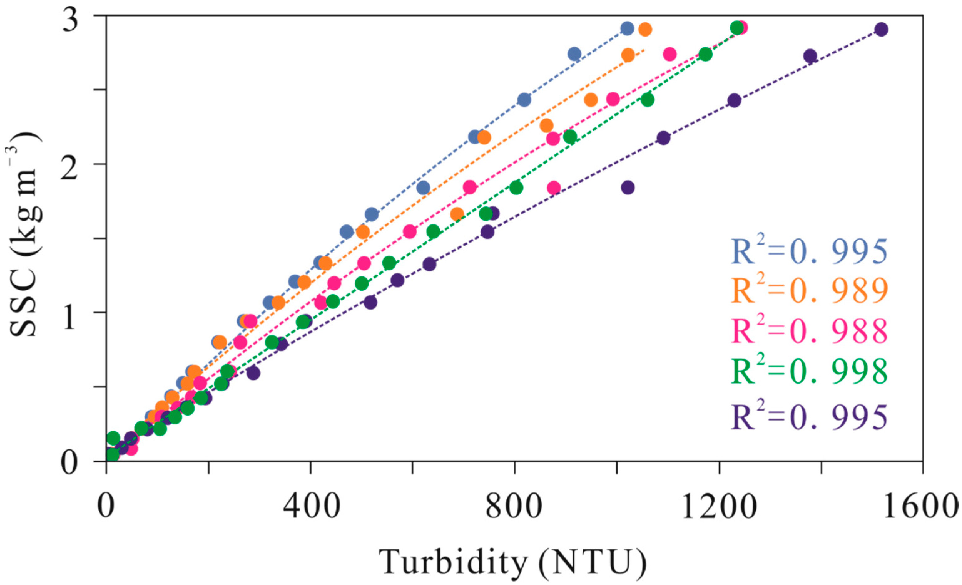
2.1. Field Observations

The observation cross-section is located at the landward boundary of turbidity maximum zone in NC with a length of 10 km (Figure 1b); the maximum difference of water depth between channel and shoal is 12.21 m (Figure 1c). The main channel and secondary channel are located in north and south edges of the transection, and the shoal is located in the middle part (Figure 1c). There are five in-situ measured stations from NC1 to NC5 northwards; tidally averaged depths of five stations are 19.63 m, 9.23 m, 7.42 m, 14.39 m and 5.82 m, respectively. The NC1 and NC4 stations are located in the main channel and secondary channel; the NC2 and NC3 stations are located on the shoal. The NC5 station is only 5 km away from the NC4 station, the current velocity and salinity at this station is strongly affected by the secondary channel. Consequently, the NC5 station is also within the range of the secondary channel.

Vertical profiles of current velocity, SSC and salinity (Figure 2) were continuously and synchronously observed for 13 h at the NC1 to NC5 stations on 9 December 2018 (spring tide in dry season). The daily averaged river discharge recorded in Datong station, which is located at the landward boundary of tidal impact, is 17,600 m³ s⁻¹. The tidal range over one flood–ebb tidal cycle at the NC1 station is 3.75 m.

The vertical profile of velocity was obtained by acoustic Doppler current profiler (ADCP, Teledyne RDI. WHR-600) with acoustic wave frequency of 600 kHz; the water depth was obtained by bottom tracking mode. During the observation, the ADCP was fixed on one side of the boat using a steel fixing frame; the transducer was at 0.5 m below the water surface. The blanking distance of the ADCP was 0.25 m, the cell size of velocity profile was 0.5 m, the sampling interval was 2 s. The optical backscatter sensor (OBS) and conductivity–temperature–depth (CTD) were winched from surface to bottom every half hour to obtain vertical profiles of turbidity and salinity with sampling intervals of 1 s. The SSC profile was estimated from the turbidity, according to the regression relation calibrated in the laboratory (Figure 3). The sediment sample used in calibration was the local suspended sediment collected during in-situ observation [25].

In order to match the temporal resolutions of SSC and salinity, the temporal variations of water depth and velocity were obtained from interpolations of measured data at every half hour, which were averages over adjacent 10 min. However, tidal deformation, water surface fluctuation and high SSC at the bottom affect the measured depth during observation [26]; temporal variations of depths at five stations obtained from interpolations are not consistent. The differences among instantaneous oscillatory depths of five stations were less than 0.5 m, which were one order of magnitude smaller than water depths of five stations. Therefore, the inconsistencies of water depth variations among five stations could not be considered.

In order to validate the longitudinal water and sediment transport, coordinate system is constructed as: x-axis is along the channel, positive seaward; y-axis is in the across-channel direction, positive to the right of the seaward direction; z-axis is positive upward. The along channel direction is identified as that of maximum tidal current variation on the cross section during a tidal cycle, which is 103° to the true north and consistent with the direction of thalweg here. The horizontal current velocity is decomposed into u component along the x-axis and v component along the y-axis according to the current direction. Flood and ebb tide durations of the profile are determined by the direction of depth-averaged current velocity, $\overline{u}$, i.e., positive value stands for ebb tide and otherwise it stands for flood tide.

2.2. Potential Energy Anomaly

The potential energy anomaly, $\varphi$ (J m⁻³), is calculated to quantify the strength of stratification in water column. For a given density profile, $\varphi$ represents the amount of energy required to mix the unit water column completely [27]. The higher value $\varphi$ is the higher energy is required for complete mixing, i.e., the stratification of water column is stronger.

$$\varphi =\left(g/h\right){{\displaystyle \int }}_{-H}^{\eta }z\left(\overline{\rho }-\rho \right)dz$$

(1)

where h is the water depth, $\eta$ is the oscillatory depth with time, H is the undisturbed water depth and h = $\eta +H$. $\overline{\rho }$ is the vertically averaged density.

$$\overline{\rho }=\left(1/h\right){{\displaystyle \int }}_0^h\rho dz$$

(2)

$\rho$ is the water density in estuary. When considering the salinity only, the $\rho$ can be calculated from the following formula [16],

$$\rho ={\rho }_0\left(1+\beta S_w\right)$$

(3)

Here, ${\rho }_0$ is the density of pure water; $\beta$ is the haline contractivity, $\beta$ = 7.8 × 10⁻⁴ [28]; $S_w$ is the salinity of water. When considering impacts of SSC and salinity, the $\rho$ can be calculated by [29],

$$\rho ={\rho }_0\left(1+\beta S_w\right)+(1-\frac{{\rho }_0\left(1+\beta S_w\right)}{{\rho }_s})\mathrm{c}$$

(4)

where ${\rho }_s$ is the sediment density, ${\rho }_s=$ 2650 kg m⁻³ and c is the SSC.

The potential energy of water increases with water depth; deeper water columns need higher energy to completely mix, i.e., the $\varphi$ is higher. In order to compare the variation processes of stratification at stations with different depth within a flood–ebb tidal cycle, the stratification ratio, $S_r$ (%), is proposed to avoid the impact of water depth at each station on $\varphi$. $S_r$ is the ratio of $\varphi$ to potential energy of the unit water column $\overline{\varphi }$ (J m⁻³), which can be regarded as the relative strength of stratification at a certain time [10]. The larger $S_r$ is, the stronger stratification of water column is;

$$S_r=\frac{\varphi }{\overline{\varphi }}·100\%.$$

(5)

Here

$$\overline{\varphi }=\frac{1}{2}\overline{\rho }gh.$$

(6)

2.3. Asymmetry Degree of Tidal Mixing

2.3.1. Eddy Viscosity and Diffusivity

The change of turbulent mixing condition within a tidal cycle is resulted from the interaction of stratification with vertical shear. The vertical gradient of density strengthen the stratification, while the enhancement of vertical shear induced by vertical gradient of current velocity can destroy the stratification. The gradient Richardson number, $R_i$, is calculated to determine how turbulence evolves in processes of shear and stratification [30].

$$R_i=\frac{N^2}{S^2}$$

(7)

where N (s⁻¹) is the buoyancy frequency. It is the frequency of the water parcel oscillate up and down around its position of neutral density in a region with linear density variation; it is defined by

$$N^2=-\frac{g}{\rho }\frac{\partial \rho }{\partial z}.$$

(8)

S (s⁻¹) is the local mean shear. If assuming that the vertical velocity gradient is much greater than the horizontal velocity gradient, it could be defined by

$$S^2={\left(\frac{\partial u}{\partial z}\right)}^2+{\left(\frac{\partial v}{\partial z}\right)}^2.$$

(9)

Therefore, $R_i$ is the ratio of the buoyancy production to the vertical shear production in turbulence. The critical value for the occurrence of shear instability in estuaries is $R_i$ = 0.25; the water column is stratified when $R_i$ > 0.25 and active mixing when $R_i$ < 0.25.

The strength of eddy diffusion caused by turbulent mixing could be quantified by the eddy viscosity ($A_v$) and diffusivity ($K_t$) [31]. The parameterization of vertical eddy viscosity is mainly based on bottom stress or gradient Richardson number. Pacanowski and Philander [32] proposed a turbulence closure model based on gradient Richardson number, where the parametric formula of $A_v$ (m² s⁻¹) reads

$$A_v=\widehat{A}{\left(1+5R_i\right)}^{-2}+{\widehat{A}}_0$$

(10)

where $\widehat{A}$ = 10⁻² m² s⁻¹ and ${\widehat{A}}_0$ = 10⁻⁴ m² s⁻¹. This closure model performs best among the lower order schemes. However, the constant $\widehat{A}$ and ${\widehat{A}}_0$ can lead to the underestimated or overestimated of $A_v$. The effects of bottom friction and non-logarithmic current velocity profile on the $A_v$ are concerned to make it more suitable in shallow areas [33].

$$\widehat{A}=C_{d}h\sqrt{{\overline{u}}^2+{\overline{v}}^2}\beta \left(z\right)$$

(11)

where $\overline{u}$ and $\overline{v}$ are the depth-averaged current velocity along x-axis and y-axis; $C_d$ is the bottom drag coefficient, the empirical value is 2.5 × 10⁻³; $\beta \left(z\right)$ is a function along the z-axis,

$$\beta \left(z\right)=\{\begin{array}{c}1, -h_0\le z\\ \frac{z+H-0.2\left(z+h_0\right)}{H-h_0}, -h\le z<-h_0\end{array}$$

(12)

$h_0$ is the thickness of the bottom boundary layer, which is setting 0.9 h here [33].

The eddy diffusivity, $K_t$ (m² s⁻¹), is related with the eddy viscosity by Prandtl-Schmidt number, $P{r}_t$.

$$K_t=\frac{A_v}{P{r}_t}.$$

(13)

Wan and Wang [34] compared several parametric formula of $P{r}_t$ and considered that the formula constructed by Karimpour and Venayagamoorthy [35] has a higher fitting degree.

$$P{r}_t=\left(1-\frac{z}{h}\right)\frac{R_i}{R_f}+\left(1-\frac{z}{h}\right)P{r}_{td0}+P{r}_{t0}.$$

(14)

Here, $P{r}_{td0}$ is the difference between the neutral turbulent Prandtl–Schmidt number at the wall ($P{r}_{tw0}\approx 1.1$) and the neutral turbulent Prandtl–Schmidt number for a homogeneous shear flow ($P{r}_{t0}=$ 0.7); $R_f$ is the flux Richardson number, $R_f=0.25\left[1-\exp \left(-7.5Ri\right)\right]$.

Without considering advection, assuming that the intensities of sediment vertical diffusion and settling are equal, the one-dimensional vertical diffusion equation of suspended sediment is as follows:

$$w_{s}c+K_0\frac{\partial c}{\partial z}=0$$

(15)

where the $w_s$ is settling velocity of suspended sediment, which is setting 0.1 mm s⁻¹ here [36]. The $K_0$ is theoretical value of eddy diffusivity. Assuming that $K_0$ is a constant in this equation, it could be compared with the depth-averaged value of $K_t$, $\overline{K_t}$, as an independent check of the calculation results of $K_t$. The resolve of c can be written as

$$\mathrm{c}=c_a{e}^{-\frac{w_s}{K_0}\left(z-z_a\right)}.$$

(16)

Here, $c_a$ is SSC at depth $z_a$; $z_a$ is setting 0.2 m on the riverbed here [37]. The equation can be transformed into

$$\ln c=\ln c_a-\frac{w_s}{K_0}\left(z-z_a\right).$$

(17)

Therefore, $\frac{w_s}{K_0}$ can be calculated by the least square method based on the measured vertical profile of SSC. The fitting profile of SSC can be obtained based on $K_0$.

2.3.2. Vertical Mixing Coefficients

As the temporal variations of vertical mixing are different among stations, the tidal mixing asymmetry is quantified by the vertical mixing coefficient, $\Omega$. $\Omega$ is dimensionless, the numerator of it is the difference between depth-averaged eddy viscosity over flood tide and over ebb tide, the denominator is the depth-averaged eddy viscosity over the whole flood–ebb tidal cycle (Equation (8) in [3]).

$$\Omega =\left({{\displaystyle \int }}_0^{T_{flood}}\overline{A_{vf}}dt-{{\displaystyle \int }}_0^{T_{ebb}}\overline{A_{ve}}dt\right)/{{\displaystyle \int }}_0^T\overline{A_v}dt$$

(18)

Here, $T_{flood}$ and $T_{ebb}$ are the flood duration and ebb duration, respectively. The durations of flood tide and ebb tide are determined by the direction of $\overline{u}$. The $\overline{A_{vf}}$, $\overline{A_{ve}}$ and $\overline{A_v}$ are the depth-averaged eddy viscosity over flood tide, ebb tide and the whole flood-ebb tidal cycle, respectively.

The value of $\Omega$ is between −1 and 1; the larger its absolute value is, the stronger asymmetry of tidal mixing is. The positive value of $\Omega$ means the regular tidal asymmetry, i.e., the vertical mixing over the flood tide is stronger than that over the ebb tide; the negative value represents reversed tidal mixing asymmetry, i.e., there is stronger vertical mixing over the ebb tide; when the value of Ω is equal to 0, the tidal mixing over the tidal cycle is symmetrical.

2.4. Longitudinal Sediment Transport

2.4.1. Longitudinal Net Water and Sediment Transports

Under the effects of bed frictions, diffusion and settling of suspended sediments and resuspension of surface sediments, the vertical variations of current velocity and SSC are significant over a flood–ebb tidal cycle [25]. In order to quantify the water and sediment transports on the surface, near-surface, bottom and near-bottom layer, the water column was vertically divided into six uniform layers. The longitudinal net water and sediment transport per unit width over a tidal cycle, $T{r}_w\left(k\right)$ (m³) and $T{r}_{sed}\left(k\right)$ (kg), are calculated on each layer, which described the vertical structure of net water and sediment transports per unit width over a tidal cycle at five stations [38]. $T{r}_w\left(k\right)$ and $T{r}_{sed}\left(k\right)$ are calculated as

$$T{r}_w\left(k\right)={{\displaystyle \int }}_0^T{U}_k·∆z_{k}dt$$

(19)

$$T{r}_{sed}\left(k\right)={{\displaystyle \int }}_0^T{U}_k·C_k·∆z_{k}dt$$

(20)

From surface to bottom, the number of the water layer, k, is from 1 to 6; the thickness $∆z_k$ of each layer is $h/6$. Within each layer, $U_k$ is the depth-averaged value of u; $C_k$ is the depth-averaged SSC. T is the period of a flood–ebb tidal cycle. Directions of $T{r}_w$ and $T{r}_{sed}$ are the same as that of u, the positive stands for seaward transport, otherwise they stand for landward transport. The sum of $T{r}_w$ or $T{r}_{sed}$ on six layer is the longitudinal net water or sediment transport per unit width at the profile.

2.4.2. Decomposition of Sediment Transport Rate

The tidally averaged longitudinal sediment transport rate per unit width, $T_s$ (kg s⁻¹), are calculated as

$$T_s=\frac{{Tr}_{sed}}{T}.$$

(21)

To analyze the contribution of tidal mixing asymmetry to the longitudinal transport of sediment within various physical processes, the $T_s$ is decomposed into several terms [39].

If the short period turbulence is ignored, current velocity u can be divided into depth-averaged term $\overline{u}$ and the deviation term at each depth from the mean value $u^{\prime }$, where

$$\overline{u}=\frac{1}{h}{{\displaystyle \int }}_0^{h}udz.$$

(22)

$\overline{u}$ can be divided into the tidally averaged term ${\overline{u}}_0$ and oscillatory term ${\overline{u}}_t$, where

$${\overline{u}}_0=\frac{1}{T}{{\displaystyle \int }}_0^T\overline{u}dt.$$

(23)

Similarly, $u^{\prime }$ can also be divided into tidally averaged term ${u^{\prime }}_0$ and oscillatory term ${u^{\prime }}_t$ at each depth. At a certain depth, u can be divided as follows:

$$u={\overline{u}}_0+{\overline{u}}_t+{u^{\prime }}_0+{u^{\prime }}_t.$$

(24)

The SSC, c, at a certain depth can also be divided as follows:

$$c={\overline{c}}_0+{\overline{c}}_t+{c^{\prime }}_0+{c^{\prime }}_t.$$

(25)

The water depth, h, can be divided into tidally averaged water depth $h_0$ and oscillatory term $h_t$ as

$$h=h_0+h_t.$$

(26)

The $T_s$ can be decomposed into seven major terms [39,40]:

$$T_s=\frac{1}{T}{{\displaystyle \int }}_0^T{{\displaystyle \int }}_0^{1}uchd\sigma dt=\underset{T_1}{\underbrace{h_0{\overline{u}}_0{\overline{c}}_0}}+\underset{T_2}{\underbrace{\langle {\overline{u}}_t{h}_t\rangle {\overline{c}}_0}}+\underset{T_3}{\underbrace{\langle h_t{\overline{c}}_t\rangle {\overline{u}}_0}}+\underset{T_4}{\underbrace{h_0\langle {\overline{u}}_t\overline{c_t}\rangle }}+\underset{T_5}{\underbrace{\langle h_t{\overline{u}}_t{\overline{c}}_t\rangle }}+\underset{T_6}{\underbrace{h_0\overline{{u^{\prime }}_0{c^{\prime }}_0}}}+\underset{T_7}{\underbrace{h_0\langle \overline{{u^{\prime }}_t{c^{\prime }}_t}\rangle }}$$

(27)

where $\sigma$ is relative depth, $\sigma =-z/h$, 0$\le \sigma \le$1 ($\sigma$ = 0 is the surface and $\sigma$ = 1 the bottom). Overbar means the depth-averaged value, and angled bracket denotes the tidal averages. The direction of sediment transport rate of each item is the same as u, i.e., positive stands for seawards and negative landwards.

T₁ is the sediment transport rate on the unit width induced by tidally averaged values of depth, velocity and SSC, i.e., the sediment transport due to Eulerian residual flow. T₂ is the sediment transport rate caused by differences of amplitude and phase between tidal oscillatory depth and tidal oscillatory velocity, i.e., the transport resulting from Stokes drift. T₁ + T₂ stands for advection transport rate. T₃ is the sediment transport rate caused by amplitude and phase differences between tidal oscillatory depth and tidal oscillatory SSC; T₄ refers to the sediment transport rate caused by amplitude and phase differences between tidal oscillatory SSC and tidal oscillatory velocity; T₅ refers to the sediment transport rate caused by the coaction of tidal oscillatory depth, tidal oscillatory velocity and tidal oscillatory SSC. T₃ + T₄ + T₅ represents sediment transport rate by tidal pumping, which is produced by the coaction of variation processes of depth, velocity and SSC within a tidal cycle [41]. T₆ is the sediment transport rate induced by the vertical structures of the tidally averaged velocity and tidally averaged SSC, resulting from landward tidally averaged velocity with high SSC near the bottom and the seaward tidally averaged velocity with low SSC near the surface, which can be interpreted as the sediment transport rate due to vertical estuary circulation. T₇ is the sediment transport rate caused by the vertical structures of tidal oscillatory velocity and tidal oscillatory SSC, induced mainly by lag in settling and diffusion of suspended sediment [10].

The vertical mixing can enhance the strength of eddy diffusion and sediment vertical diffusion, increase the SSC on the upper layer and result in pumping of sediment with the tidal current. Therefore, the contribution of tidal mixing asymmetry on tidally averaged sediment transport rate is included in the T₄ term of tidal pumping, which is caused by amplitude and phase differences between SSC and current [12].

2.4.3. Decomposition of Sediment Flux

To analyze the mechanism of suspended sediment transport on the vertical profile within a tidal cycle, the longitudinal tidally averaged sediment flux, <uc> (kg m⁻² s⁻¹), is decomposed into two parts [10,41]

$$<uc>=u_0{c}_0+<u_t{c}_t>$$

(28)

where $u_0$ and $c_0$ are tidally averaged velocity and SSC. $u_0{c}_0$ is the advection sediment flux caused by the Eulerian residual flow and tidally averaged SSC; $<u_t{c}_t>$ is the sediment flux caused by the coaction of tidal oscillatory velocity and tidal oscillatory SSC, i.e., the sediment transport flux induced by tidal pumping.

3. Result

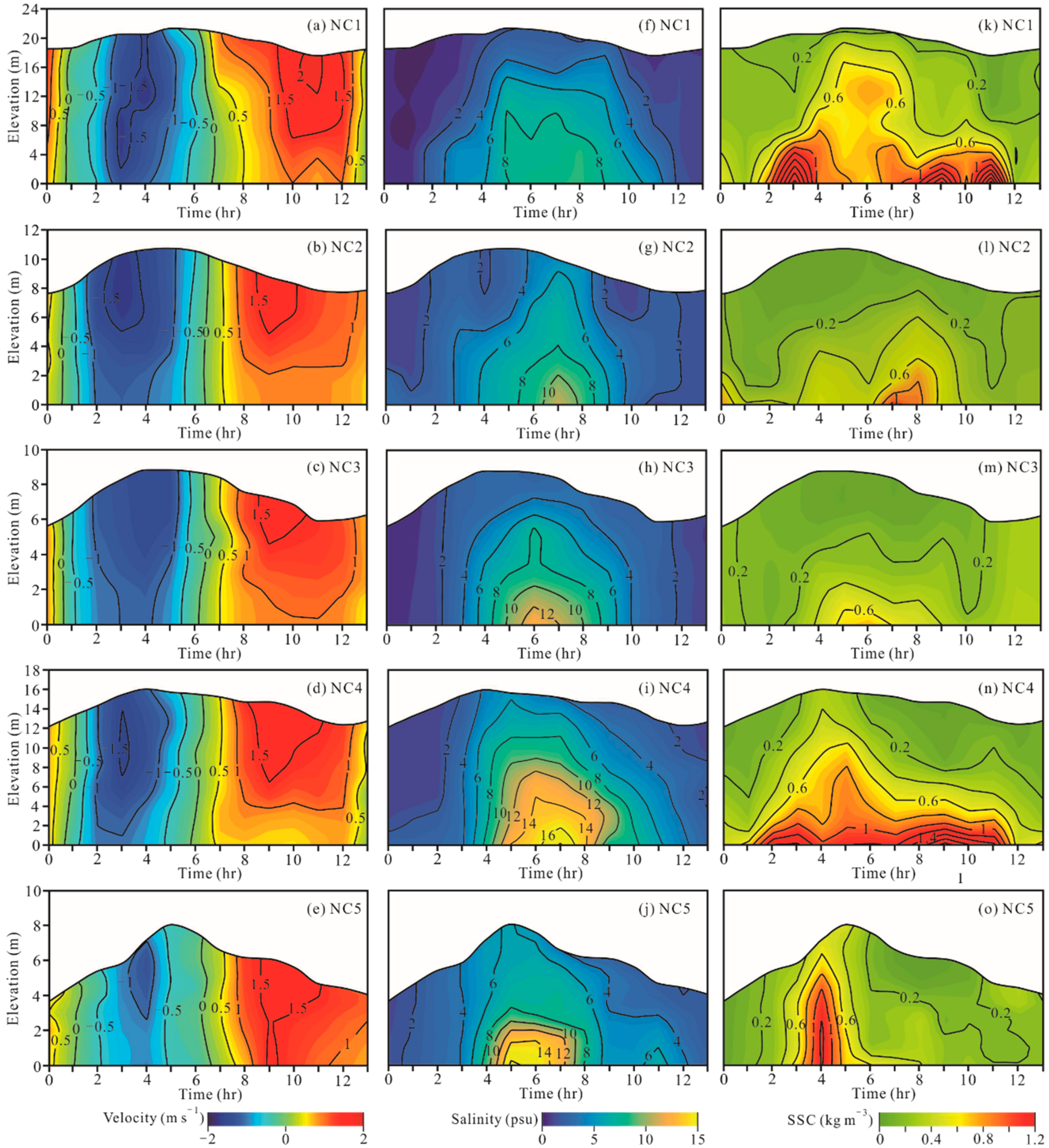
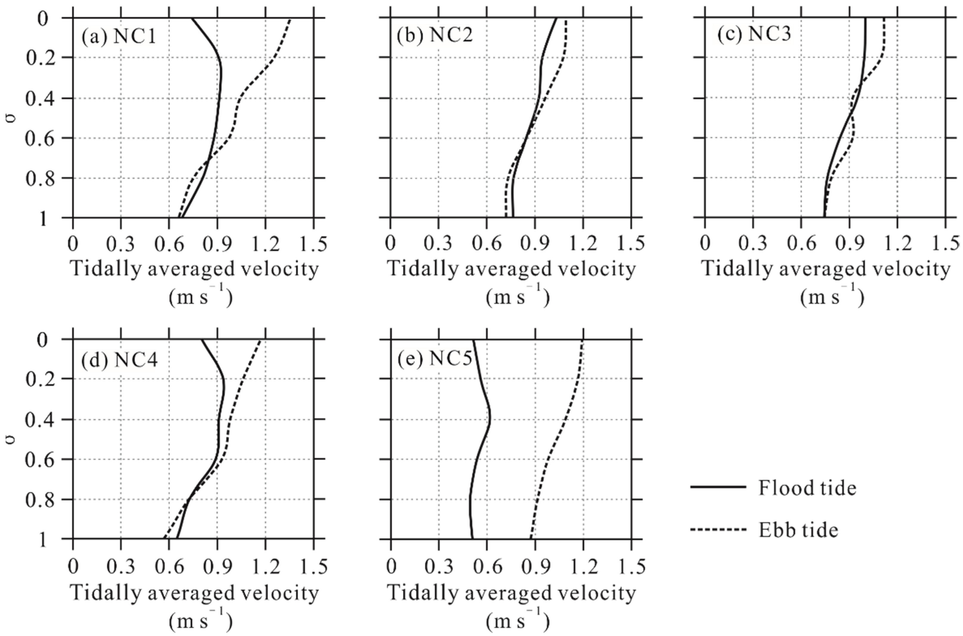
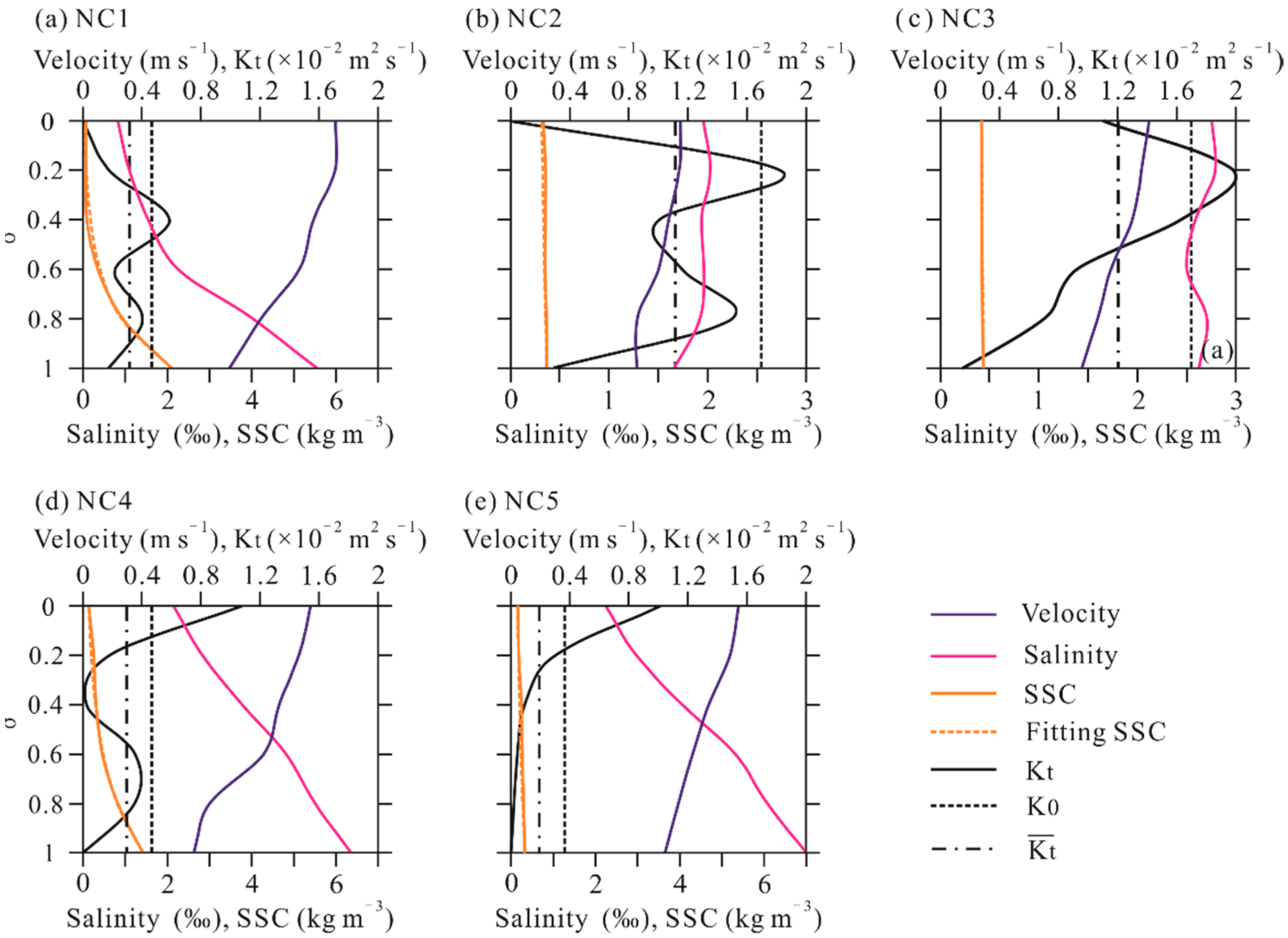
3.1. Lateral Variations of Velocity and Salinity

During the spring tide in the dry season, ebb durations were greater than flood in five stations; flood durations decreased and ebb durations increased northwards along the cross section. The ebb tidally averaged velocities were larger than flood tidally averaged at five stations. At the NC1 and NC4 stations with deeper depth, flood and ebb tidally averaged velocities were higher than the other three stations (

Table 1. Characteristic values of current velocity at NC1 to NC5 stations.

Stations	Tidal-Mean Depth (m)	Flood Tide			Ebb Tide
		Flood Durations (h)	Mean Velocity * (m s−1)	Maximum Velocity * (m s−1)	Ebb Durations (h)	Mean Velocity * (m s−1)	Maximum Velocity * (m s−1)
NC1	19.63	5.7	0.95	1.50	6.6	1.00	1.59
NC2	9.23	5.9	0.84	0.95	6.7	0.90	1.11
NC3	7.42	5.7	0.84	1.30	7.2	0.93	1.31
NC4	14.39	5.2	0.88	1.38	7.3	1.04	1.58
NC5	5.82	5.3	0.54	1.20	7.7	0.91	1.42

* Depth-averaged value.

). Ebb tidally averaged velocities were larger than flood tidally averaged on surface and smaller than flood tidally averaged on bottom at the NC1 to NC4 stations (Figure 4a–d), and it was larger than flood tidally averaged on each layer at the NC5 station (Figure 4e).

Tidally averaged salinities at the NC1 to NC5 stations were 3.61 (unit: psu, the same below), 3.81, 4.03, 5.71 and 4.67, respectively. At these stations, ranges of salinity variations on the bottom layer were significantly larger than that on the surface layer over a tidal cycle, and the appearance of salinity peak slightly lagged behind the flood slack (Figure 2f–j). The ranges of salinity variations on the bottom layer rose from 0.55–9.20 at the NC1 station to 1.78–16.17 at the NC5 station. Tidally averaged salinities and ranges of bottom-layer salinity variation increased northwards along the cross section.

3.2. Temporal Variation of Stratification

The stratification ratio, $S_r$, considering the impacts of SSC and salinity was greater than that considering the impact of salinity only; the SSC increased the stratification degree of water columns. However, the SSC did not change the variation trend of $S_r$ within a tidal cycle (Figure 5). Because this study mainly discusses the impact of mixing and stratification on SSC and sediment transport, the remainder contents only describe the variation of $S_r$ considering salinity.

The $S_r$ at five stations was less than 0.01% and remained at a lower value during the early flood; the water columns were weakly stratified. After the maximum flood, the $S_r$ increased rapidly and reached the peak around the time of the flood slack. During the early ebb tide, the $S_r$ decreased gradually.

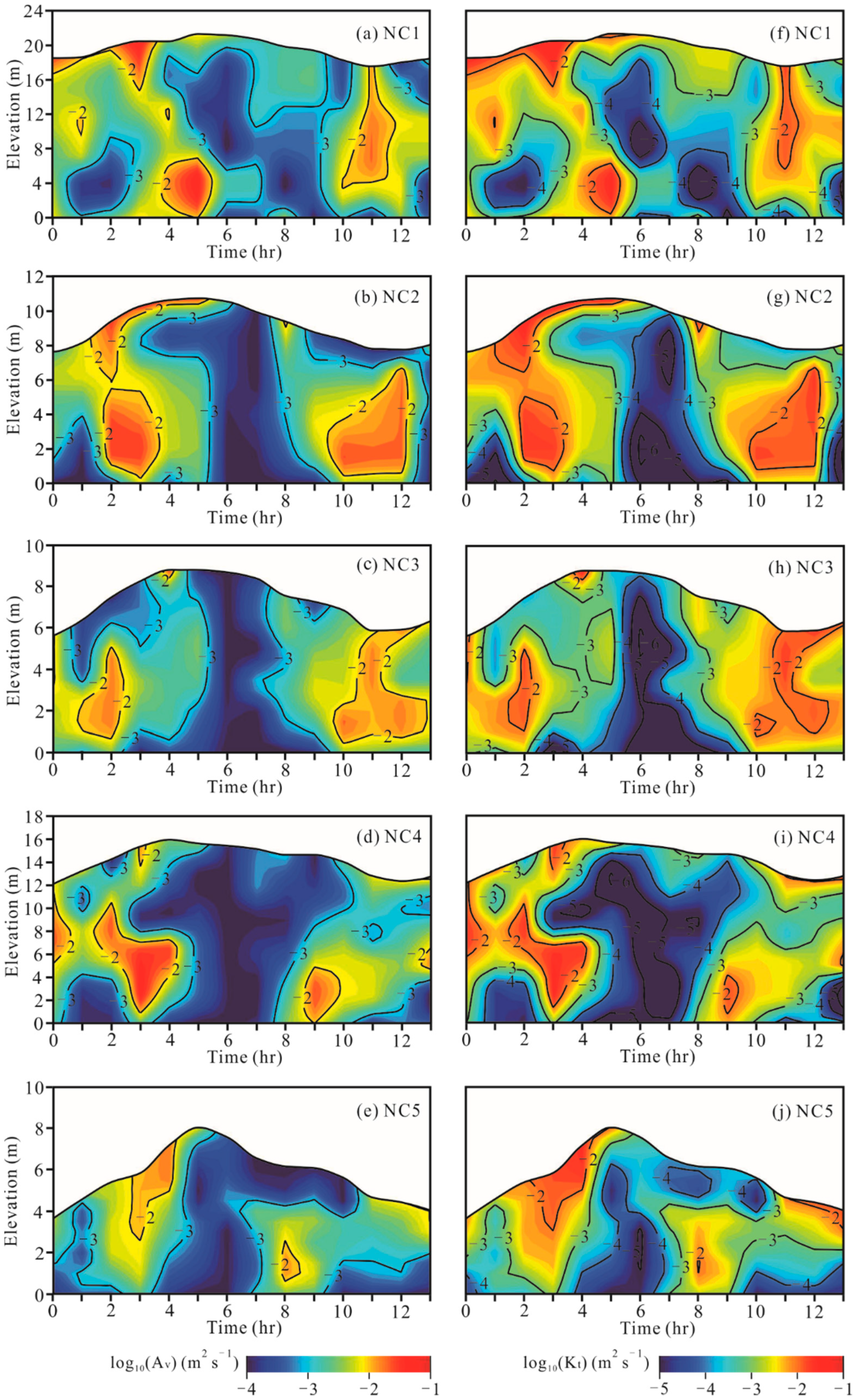
3.3. Temporal Variations of Eddy Viscosity and Diffusivity

On the transection, the eddy viscosity, $A_v$, ranged from 10⁻⁴ to 10⁻¹ m² s⁻¹, and the eddy diffusivity, $K_t$, ranged from 10⁻⁵ to 10⁻¹ m⁻² s⁻¹; the variation of $K_t$ was consistent with $A_v$ (Figure 6).

During the early flood, the mean shear square, S², increased with flood current velocity (Figure 7). The buoyancy frequency square, N², increased slightly, resulting from the lag of salinity rise; the stratification was weak. The gradient Richardson number,$R_i$, was less than 0.25; strong vertical shear enhanced the mixing in water columns with higher $A_v$, which induced stronger eddy diffusion with higher $K_t$ (Figure 6). Within the maximum flood and maximum ebb, the stronger stratification with higher N² restrained the vertical mixing and eddy diffusion;$R_i$ was higher than 0.25, $A_v$ and $K_t$ decreased and reached the minimum at the flood slack. After the maximum ebb, with the reduction in salinity and decrease in stratification, the vertical mixing and eddy diffusion were strengthened under the effect of vertical shear; values of $A_v$ and $K_t$ increased.

The depth-averaged eddy viscosity $\overline{A_v}$ and depth-averaged eddy diffusivity $\overline{K_t}$ were larger during the early flood and after the maximum ebb, which were smaller within the maximum flood to the early ebb. The variations of $\overline{A_v}$ and $\overline{K_t}$ were opposite to the $S_r$ (Figure 5).

3.4. Lateral Variations of Tidal Mixing Asymmetry

Over one flood–ebb tidal cycle, vertical mixing coefficients, $\Omega$, of the NC 1, NC4 and NC5 stations in channel, were 0.12, 0.16 and 0.06, respectively; the vertical mixing during flood tide was stronger than that during ebb tide, which showed regular tidal mixing asymmetry. The $\Omega$ of the NC2 and NC3 stations on the shoal were −0.02 and −0.27; the vertical mixing during flood tide was weaker than that during ebb tide, which showed reversed tidal mixing asymmetry.

3.5. Longitudinal Sediment Transport

3.5.1. Lateral Variations of SSC

The tidally averaged SSC at the NC1, NC4 and NC5 stations in channel were 0.44 kg m⁻³, 0.46 kg m⁻³ and 0.30 kg m⁻³. Meanwhile, the tidally averaged SSC at the NC2 and NC3 stations were 0.25 kg m⁻³ and 0.21 kg m⁻³. The tidally averaged SSC increased with the water depth.

During flood tide, depth-averaged SSC at the NC1 to NC5 stations gradually increased. After the flood slack, depth-averaged SSC decreased and remained at the tidally averaged values. After the maximum ebb, i.e., 11 h after the beginning of observation, depth-averaged SSC at the NC1, NC4 and NC5 stations in the channel decreased to 0.18 kg m⁻³, 0.22 kg m⁻³ and 0.06 kg m⁻³, which were lower than tidally averaged values (Figure 8a–c). Meanwhile, depth-averaged SSC at the NC2 and NC3 stations on the shoal increased to 0.40 kg m⁻³ and 0.35 kg m⁻³, which were larger than tidally averaged values (Figure 8b,d).

Therefore, at the NC1, NC4 and NC5 stations in channel, flood tidally averaged SSC were larger than ebb tidally averaged. At the NC1 station, the tidally averaged SSC were 0.48 kg m⁻³ over flood tide and 0.42 kg m⁻³ over ebb tide. At the NC4 station, the tidally averaged SSC were 0.50 kg m⁻³ over flood tide and 0.43 kg m⁻³ over ebb tide. At the NC5 station, the flood tidally averaged SSC was 0.45 kg m⁻³ and ebb tidally averaged SSC was 0.20 kg m⁻³. At the NC1 and NC4 stations, the flood tidally averaged SSC above 0.8 h were larger than the ebb tidally averaged SSC. By contrast, near the bottom layer, the flood tidally averaged SSC were smaller than the ebb tidally averaged SSC (Figure 9a,d). At the NC5 station, the flood tidally averaged SSC was larger than the ebb tidally averaged SSC on each layer (Figure 9e).

At the NC2 and NC3 stations, located on the shoal, the flood tidally averaged SSC were larger than that of the ebb tidally averaged SSC. At the NC2 station, the flood and ebb tidally averaged SSC were 0.21 kg m⁻³ and 0.29 kg m⁻³. At the NC3 stations, the flood and ebb tidally averaged SSC were 0.17 kg m⁻³ and 0.25 kg m⁻³. At the NC2 and NC3 stations, the ebb tidally averaged SSC were larger than the flood tidally averaged SSC on each layer (Figure 9b,c).

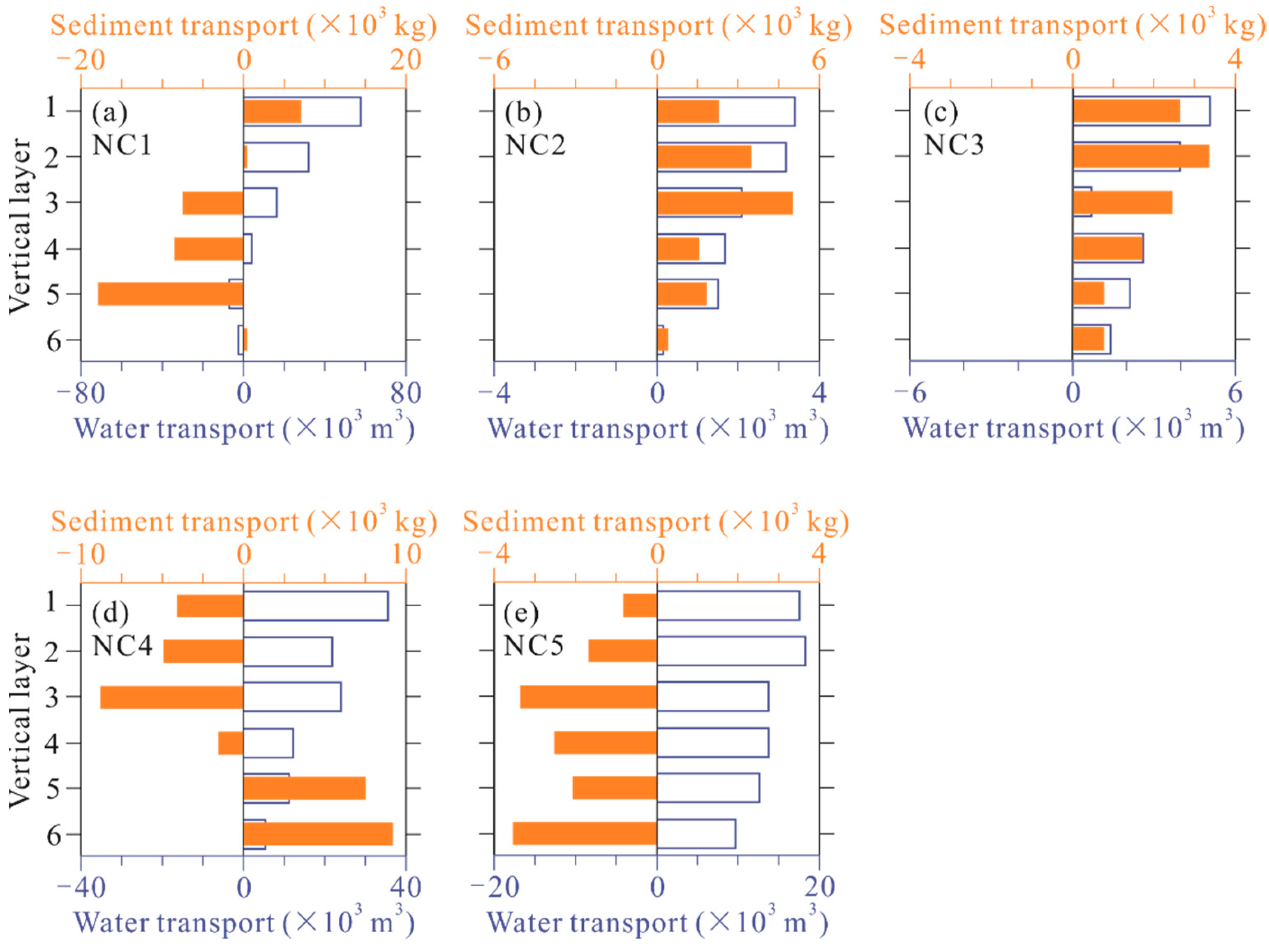
3.5.2. Lateral Variations of Longitudinal Net Water and Sediment Transports

Over a flood–ebb tidal cycle, the longitudinal net water transports $T{r}_w$ at the NC1 to NC5 stations were 1.00 × 10⁵ m³, 1.21 × 10⁴ m³, 1.61 × 10⁴ m³, 1.11 × 10⁵ m³ and 8.62 × 10⁴ m³, respectively. Except for the landward water transport on the bottom layer at the NC1 station, located in the main channel near the south bank, $T{r}_w$ on each layer at all other stations were seaward (hollow bars in Figure 10a–e).

The longitudinal net sediment transports $T{r}_{sed}$ at the NC1 to NC5 stations were −2.61 × 10⁴ kg, 1.46 × 10⁴ kg, 1.17 × 10⁴ kg, −2.82 × 10³ kg and −1.40 × 10⁴ kg, respectively. $T{r}_{sed}$ at the NC1, NC4 and NC5 stations were landward. However, $T{r}_{sed}$(1), $T{r}_{sed}$(2) and $T{r}_{sed}$(6) at the NC1 station, i.e., net sediment transports on layers above 0.4 h and below 0.8 h were seaward. $T{r}_{sed}$(5) and $T{r}_{sed}$(6) at the NC4 station, i.e., net sediment transports on layers below 0.6 h, were also seaward. $T{r}_{sed}$ on other layers at the NC1, NC4 and NC5 stations were landward and on each layers at the NC2 and NC3 stations were seaward (filled bars in Figure 10a–e).

In conclusion, the lateral variations of $T{r}_{sed}$ on the cross section were significantly different with that of $T{r}_w$. $T{r}_w$ were mainly seaward on the whole transection; $T{r}_{sed}$ were mainly landward in the channel and seaward on the shoal.

3.5.3. Tidally Averaged Longitudinal Sediment Transport Rate

The tidally averaged sediment transport rates caused by Eulerian flow, T₁, were higher than the landward transport rates, T₂, caused by Stokes drift, at five stations. Advection transport rates T₁ + T₂ were positive, which showed seaward transports on the whole transection (

Table 2. Decomposed longitudinal tidally averaged sediment transport rates per unit width (kg s⁻¹) at NC1 to NC5 stations.

Station	T1	T2	T3	T4	T5	T6	T7	T1 + T2	T3 + T4 + T5	${\mathit{T}}_{\mathit{s}}$
NC1	1.31	−0.43	0.02	−1.10	−0.06	−0.54	−0.20	0.88	−1.14	−0.59
NC2	0.19	−0.12	0.00	0.18	0.01	−0.02	0.01	0.07	0.19	0.32
NC3	0.31	−0.22	0.00	0.16	−0.02	−0.02	0.03	0.09	0.14	0.25
NC4	1.08	−0.28	0.02	−0.65	−0.06	−0.36	−0.13	0.80	−0.69	−0.06
NC5	0.70	−0.15	0.05	−0.78	−0.12	−0.03	0.02	0.55	−0.85	−0.30

). The advection transport rates of the NC1, NC4 and NC5 stations in the channel were significantly higher than those at the NC2 and NC3 stations on the shoal.

At the stations NC1, NC4 and NC5, sediment transport rates induced by tidal pumping, i.e., T₃ + T₄ + T₅, were negative, which showed landward transports. At the NC2 and NC3 stations, sediment transport rates caused by tidal pumping were seaward. Sediment transport rates by tidal pumping were landward in channel and seaward on the shoal, which were similar with the total sediment transport rates $T_s$. In three terms of the sediment transport rate induced by tidal pumping, the value of T₄ was significantly higher than the other two items at each stations; the coaction of SSC and current velocity made a more significant contribution to the sediment transport rate. The contributions of T₄ to T₃ + T₄ + T₅ were from 91.8% to 114.3% at five stations; the magnitude and direction of sediment transports induced by tidal pumping mainly depend on T₄ item.

Furthermore, T₆ values at five stations were negative; the sediment transport rates driven by gravitation circulation were landward. T₇ were negative at the stations NC1 and NC4, and positive at other stations. Except for the NC1 and NC4 stations with deep depth, the contributions of T₆ and T₇ terms at other three stations could be ignored because of the relatively small values.

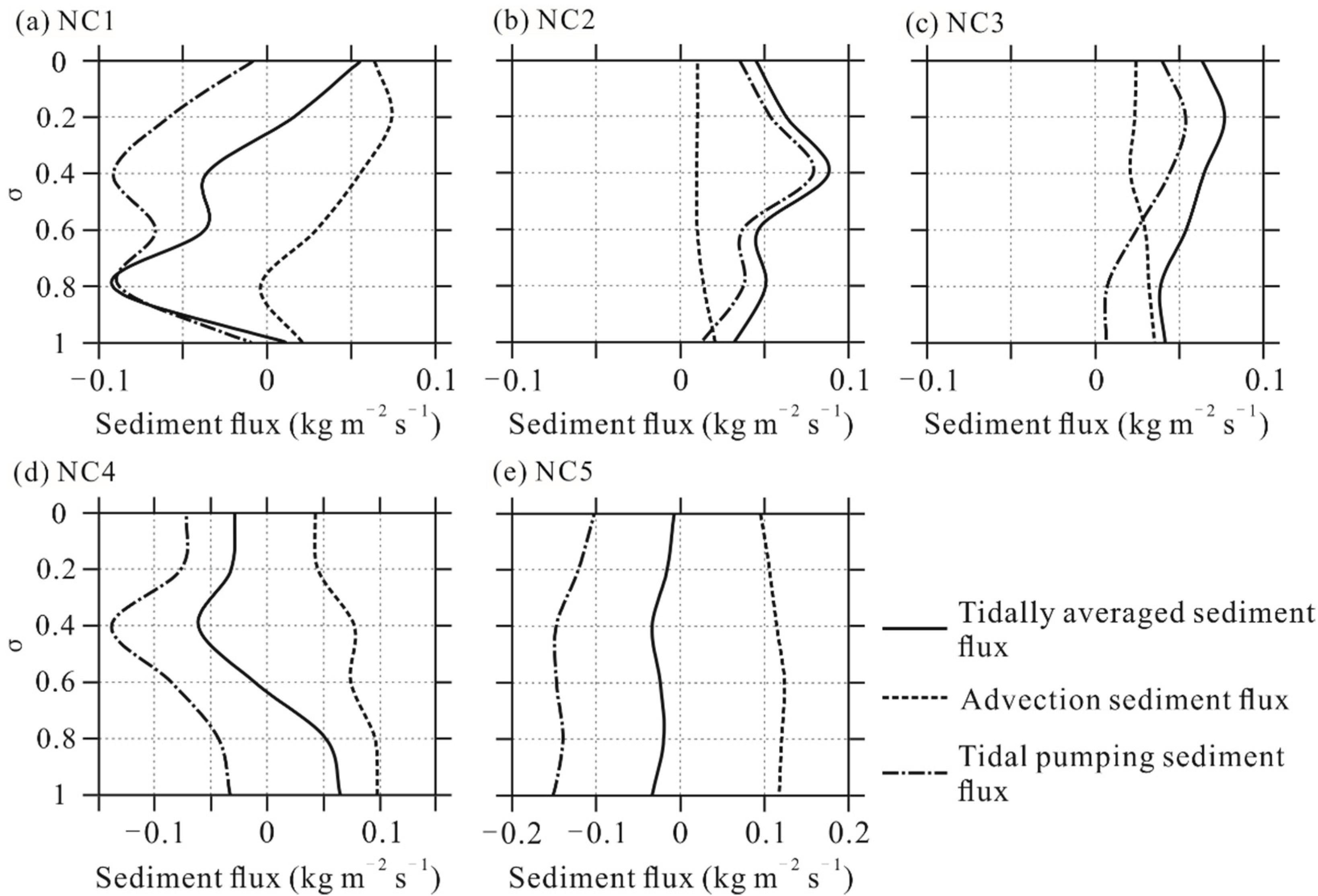
3.5.4. Tidally Averaged Longitudinal Sediment Flux

The vertical profiles of longitude tidally averaged sediment flux, <uc>, were similar with $T{r}_{sed}$ (Figure 11). The advection sediment flux, $u_0{c}_0$, were seaward at five stations; the tidal pumping sediment flux $<u_t{c}_t>$ were landward at the NC1, NC4 and NC5 stations in the channel and seaward at the NC2 and NC3 stations on the shoal.

4. Discussion

4.1. Mechanism behind Lateral Variations of Tidal Mixing Asymmetry

The transaction was located at the landward boundary of the turbidity maximum zone in the Yangtze Estuary. The barotropic pressure gradient caused by the huge river discharge of the Yangtze River made the variation range of salinity on surface layer significantly less than bottom within a tidal cycle [42]. With the variation of salinity on bottom, the stratification of water columns increased during flood tide and decreased during ebb tide (Figure 2 and Figure 5). Stronger stratification restrained the vertical mixing caused by vertical shear and made the $R_i$ greater than the critical value, resulting in weaker vertical mixing and eddy diffusion. During the period of weaker stratification, the vertical shear made the $R_i$ less than critical value, resulting in stronger turbulent diffusion [19,43].

However, after the maximum ebb, the reduction in stratification at the stations NC1, NC4 and NC5 in channel lagged behind the stations NC2 and NC3 on the shoal (Figure 5). From the 10th to 12th hour after the beginning of observation, $S_r$ at three stations in the channel ranged from 0.00% to 0.09%; the $R_i$ were greater than 0.25; the $\overline{A_v}$ and $\overline{K_t }$ still maintained at a lower value (Figure 5 and Figure 7). Therefore, the strength of vertical mixing over ebb tide was lower than that over flood tide, showing regular tidal mixing asymmetry.

Meanwhile, at the NC2 and NC3 stations on the shoal, the stratification decreased rapidly; $S_r$ at three stations in channel ranged from 0.00% to 0.03%. The strong ebb current enhanced the vertical shear and turbulent mixing, the $R_i$ reduced to below 0.25 and the $\overline{A_v}$ and $\overline{K_t }$ increased to the values closing to the beginning of flood tide (Figure 5 and Figure 7). The strength of vertical mixing over ebb tide was higher than that over flood tide, showing reversed tidal mixing asymmetry.

Taking the 11th hour after the beginning of observation as an example, the salinities on the surface layer at five stations were similar, but the salinities on the bottom layer at the NC1, NC4 and NC5 stations were higher than the NC2 and NC3 stations. The $S_r$ ranged from 0.06% to 0.07% at three stations in the channel and around 0.00% on the shoal. The $\overline{K_t}$ were 0.0031 m² s⁻¹, 0.0029 m² s⁻¹ and 0.0019 m² s⁻¹ at the NC1, NC4 and NC5 stations, respectively; they were 0.011 m² s⁻¹ and 0.012 m² s⁻¹ at the NC2 and NC3 stations; the $\overline{K_t}$ in two stations on the shoal were an order of magnitude larger than three stations in the channel (Figure 5). The fitting results of the one-dimensional equation showed that the fitting vertical profile of SSC was close to the measured. The theoretical value of eddy diffusivity $K_0$ was closed to the $\overline{K_t}$; they were 0.004 m² s⁻¹, 0.0042 m² s⁻¹ and 0.0039 m² s⁻¹ at the NC1, NC4 and NC5 stations, respectively, and were 0.017 m² s⁻¹ both at the NC2 and NC3 stations; the $\overline{K_t}$ in two stations on the shoal were also an order of magnitude larger than three stations in the channel (Figure 12).

4.2. Impact of Tidal Mixing Asymmetry on Longitudinal Net Sediment Transport

The eddy diffusion caused by the vertical mixing could transport upward the higher concentration sediment near the bottom and increase the SSC in the upper layer of water columns, while the restraint of stratification on eddy diffusion makes sediment accumulate near the bottom [22,25]. Taking the 11th hour after the beginning of observation as an example again, resulting from weaker eddy diffusion, the ratios of SSC on the surface to bottom layer ranged from 0.03 to 0.34 at the NC1, NC4 and NC5 stations in the channel, which were less than 0.74 to 0.76 at the NC2 and NC3 stations on the shoal; the SSC on surface layer ranging from 0.06 kg m⁻³ to 0.09 kg m⁻³ at three stations in channel were also less than 0.19 kg m⁻³ to 0.23 kg m⁻³ at two stations on the shoal.

At the stations NC1, NC4 and NC5 in the channel, the effect of regular tidal asymmetry resulted in the landward T₃ + T₄ + T₅ and $T_s$ (Table 2). With stronger eddy diffusion increasing the SSC during the early flood (Figure 2), the flood tidally averaged SSC above 0.8 h were higher than ebb tidally averaged SSC (Figure 9a,d,e). Therefore, the depth-averaged SSC were larger than the tidally averaged SSC significantly during the early flood tide; the averaged value of tidal oscillatory SSC, ${\overline{c}}_t$, over the flood tide were larger than it over the ebb tide (Figure 8a,d,e). Under the transportation of the flood current [12,22], the T₄ term was landward. Because the landward T₃ + T₄ + T₅ was higher than seaward transport rate by advection, T₁ + T₂, the $T_s$ and net sediment transport $T{r}_{sed}$ were landward in the channel.

At the NC2 and NC3 stations on the shoal, the effect of reversed tidal asymmetry resulted in the seaward T₃ + T₄ + T₅ and seaward $T_s$ (Table 2). The stronger eddy diffusion increased the SSC after the maximum ebb (Figure 2); the ebb tidally averaged SSC was higher than flood tidally averaged SSC (Figure 9b,c). As the depth-averaged SSC was larger than the tidally averaged SSC significantly after the maximum ebb, the averaged value of ${\overline{c}}_t$ over ebb tide was larger than it over flood tide (Figure 8b,c). Under the transportation of ebb current, the directions of T₄ and T₃ + T₄ + T₅ were seaward. They were superimposed with the seaward T₁ + T₂, resulting in the seaward $T_s$ and $T{r}_{sed}$ on the shoal.

In the last two decades, due to the reduction in sediment from the basin and the constructions of the reclamations in estuary, there were erosion in the channel and deposition on the shoal in the NC [24]. The numerical simulation results in the NC showed that, during spring tide, due to the deepening and narrowing of the channel in turbidity maximum zone, stratification was enhanced and the maximum stratification occurred near the maximum ebb in main channel; the increase in the stratification was less on the shoal resulting from the higher bottom friction [44]. Therefore, in turbidity maximum zone of NC, the landward sediment transport induced by tidal pumping was enhanced in the main channel, and the lateral variation of the sediment transport was intensified.

4.3. Impacts of Advection and Resuspension on Longitudinal Net Sediment Transport

The $T{r}_{sed}\left(1\right)$ at the NC1 station, i.e., the sediment transports on the layers near the surface in the main channel, were seaward. The $T{r}_{sed}\left(6\right)$ at the NC1 and NC4 stations, i.e., the sediment transports on the layers near the bottom in main and secondary channels, were also seaward. (Figure 10a,d). This is inconsistent with the distribution of the net sediment transport on the transection.

Resulted from the large river discharge, there is strong seaward water transport near the surface within the main channel in the Yangtze estuary [21]. The $T{r}_w\left(1\right)$ at the NC1 station was 5.76 × 10⁴ m³, twice that at the NC4 station located in the secondary channel. The ebb tidally averaged velocity was 1.36 m s⁻¹ at the NC1 station, which was higher than other stations significantly (Figure 4). The seaward $u_0{c}_0$ above 0.2 h was larger than landward $<u_t{c}_t>$ (Figure 11a). The strong advection transport induced the seaward $<uc>$ and $T{r}_{sed}\left(1\right)$ at the NC1 station.

At the NC1 and NC4 stations with deeper water depth, the resuspension of sediment on riverbed increased the SSC on bottom (the sixth layer) during ebb tide and resulted in the seaward $T{r}_{sed}\left(6\right)$. At the NC1 and NC4 stations with deeper water depth, the maximum depth-averaged ebb current velocity and ebb tidally averaged velocity were higher than those of other stations (Table 1). Due to the strong ebb current, SSC on bottom reached the peak at the maximum ebb, which were 2.11 kg m⁻³ and 1.84 kg m⁻³ (Figure 2k,n). The ebb tidally averaged SSC on bottom were higher than the flood tidally averaged (Figure 9a,d); the resuspension of sediment was obvious. During the whole tidal cycle, the SSC on bottom maintained at the higher value, which made the $u_0{c}_0$ larger than $<u_t{c}_t>$ (Figure 11d); the $<uc>$ and $T{r}_{sed}$(6) were seaward.

5. Conclusions

The key message of this study is that tidal mixing asymmetry at the landward boundary of the turbidity maximum zone in a time-dependent salt wedge estuary is sensitive to lateral variation of bathymetry and can thus affect variations of eddy diffusion and SSC during a flood–ebb tidal cycle, which causes the landward net sediment transport in the channel and seaward sediment transport on the shoal. The main conclusions are listed below.

(1) With the variation of salinity on bottom, the stratification of water columns increased during the flood tide and decreased during the ebb tide. After the maximum ebb, the reduction in stratification at the stations NC1, NC4 and NC5 in the channel lagged behind the stations NC2 and NC3 on the shoal. The stronger stratification restrained the turbulent mixing caused by vertical shear in the channel; the vertical mixing over the ebb tide was lower than that over flood tide, showing regular tidal mixing asymmetry. Meanwhile, the stratification decreased rapidly on the shoal; the vertical mixing over the ebb tide was higher than that over the flood tide resulting from the vertical shear, showing reversed tidal mixing asymmetry.

(2) At the NC1, NC4 and NC5 stations in the channel, the stronger eddy diffusion during flood tide caused by vertical mixing transported sediment upward from the bottom layer; the flood tidally averaged SSC were higher than ebb tidally averaged. Higher concentration sediment produced higher landward tidally averaged sediment transport rates by tidal pumping under the transportation of the flood tidal current; net sediment transports were landward. At the NC2 and NC3 stations on the shoal, the flood tidally averaged SSC were lower than the ebb tidally averaged due to the reversed tidal mixing asymmetry. The sediment transport rates by tidal pumping and net sediment transports were seaward.

(3) Due to large seaward water transport, the seaward tidally averaged sediment flux and $T{r}_{sed}$ on the surface of the main channel were induced by advection. In the main and secondary channel, strong ebb velocity induced sediment resuspension; the SSC near the bottom maintained at a high degree during the whole tidal cycle. The seaward sediment flux caused by advection increased, resulting in the seaward tidally averaged sediment flux and $T{r}_{sed}$ on bottom.

References

1. Simpson, J.H.; Brown, J.; Matthews, J.; Allen, G. Tidal Straining, Density Currents, and Stirring in the Control of Estuarine Stratification. Estuaries 1990, 13, 125–132. [Google Scholar] [CrossRef]
2. Jay, D.A.; Musiak, J.M. Internal tidal asymmetry in channel flows. Origins and consequences. In Mixing Processes in Estuaries and Coastal Seas, Coastal Estuarine Studies Series; AGU: Washington, DC, USA, 1996; Volume 50, pp. 211–249. [Google Scholar] [CrossRef]
3. Cheng, P.; Valle-Levinson, A.; De Swart, H.E. A numerical study of residual estuarine circulation induced by asymmetric tidal mixing in tidally dominated estuaries. J. Geophys. Res. Oceans 2011, 116, C01017. [Google Scholar] [CrossRef] [Green Version]
4. Burchard, H.; Baumert, H. The Formation of Estuarine Turbidity Maxima Due to Density Effects in the Salt Wedge. A Hydrodynamic Process Study. J. Phys. Oceanogr. 1998, 28, 309–321. [Google Scholar] [CrossRef]
5. Scully, M.E.; Friedrichs, C.T. Sediment pumping by tidal asymmetry in a partially mixed estuary. J. Geophys. Res. Oceans 2007, 112, C07028. [Google Scholar] [CrossRef] [Green Version]
6. Geyer, W.R. The Importance of Suppression of Turbulence by Stratification on the Estuarine Turbidity Maximum. Estuaries 1993, 16, 113–125. [Google Scholar] [CrossRef]
7. Scully, M.E.; Friedrichs, C.T. The influence of asymmetries in overlying stratification on near-bed turbulence and sediment suspension in a partially mixed estuary. Ocean Dyn. 2003, 53, 208–219. [Google Scholar] [CrossRef]
8. Wan, Y.; Gu, F.; Wu, H.; Roelvink, D. Hydrodynamic evolutions at the Yangtze Estuary from 1998 to 2009. Appl. Ocean Res. 2014, 47, 291–302. [Google Scholar] [CrossRef]
9. Sanford, L.P.; Suttles, S.E.; Halka, J.P. Reconsidering the Physics of the Chesapeake Bay Estuarine Turbidity Maximum. Estuaries 2001, 24, 655–669. [Google Scholar] [CrossRef]
10. Li, L.; He, Z.; Xia, Y.; Dou, X. Dynamics of sediment transport and stratification in Changjiang River Estuary, China. Estuar. Coast. Shelf Sci. 2018, 213, 1–17. [Google Scholar] [CrossRef]
11. Whitney, M.M.; Codiga, D.L.; Ullman, D.S.; McManus, P.M.; Jiorle, R. Tidal Cycles in Stratification and Shear and Their Relationship to Gradient Richardson Number and Eddy Viscosity Variations in Estuaries. J. Phys. Oceanogr. 2012, 42, 1124–1133. [Google Scholar] [CrossRef]
12. Scully, M.E.; Friedrichs, C.T. The importance of tidal and lateral asymmetries in stratification to residual circulation in partially mixed estuaries. J. Phys. Oceanogr. 2007, 37, 1496–1511. [Google Scholar] [CrossRef] [Green Version]
13. Fugate, D.C.; Friedrichs, C.T.; Sanford, L.P. Lateral dynamics and associated transport of sediment in the upper reaches of a partially mixed estuary, Chesapeake Bay, USA. Cont. Shelf Res. 2007, 27, 679–698. [Google Scholar] [CrossRef]
14. Basdurak, N.B.; Valle-Levinson, A.; Cheng, P. Lateral structure of tidal asymmetry in vertical mixing and its impact on exchange flow in a coastal plain estuary. Cont. Shelf Res. 2013, 64, 20–32. [Google Scholar] [CrossRef]
15. Ralston, D.K.; Geyer, W.R.; Warner, J.C. Bathymetric controls on sediment transport in the Hudson River estuary: Lateral asymmetry and frontal trapping. J. Geophys. Res. Oceans 2012, 117, C10013. [Google Scholar] [CrossRef] [Green Version]
16. Geyer, W.R.; MacCready, P. The Estuarine Circulation. Annu. Rev. Fluid Mech. 2014, 46, 175–197. [Google Scholar] [CrossRef]
17. Giddings, S.N.; Fong, D.A.; Monismith, S.G. Role of straining and advection in the intratidal evolution of stratification, vertical mixing, and longitudinal dispersion of a shallow, macrotidal, salt wedge estuary. J. Geophys. Res. Oceans 2011, 116, C03003. [Google Scholar] [CrossRef] [Green Version]
18. Burchard, H.; Schuttelaars, H.M.; Ralston, D.K. Sediment Trapping in Estuaries. Annu. Rev. Mar. Sci. 2018, 10, 371–395. [Google Scholar] [CrossRef]
19. Pu, X.; Shi, J.Z.; Hu, G.-D.; Xiong, L.-B. Circulation and mixing along the North Passage in the Changjiang River estuary, China. J. Mar. Syst. 2015, 148, 213–235. [Google Scholar] [CrossRef]
20. Cheng, H.; Chen, J.; Chen, Z.; Ruan, R.; Xu, G.; Zeng, G.; Zhu, J.; Dai, Z.; Chen, X.-Y.; Gu, S.; et al. Mapping Sea Level Rise Behavior in an Estuarine Delta System: A Case Study along the Shanghai Coast. Engineering 2018, 4, 156–163. [Google Scholar] [CrossRef]
21. Jiang, C.; de Swart, H.E.; Li, J.; Liu, G. Mechanisms of along-channel sediment transport in the North Passage of the Yangtze Estuary and their response to large-scale interventions. Ocean Dyn. 2013, 63, 283–305. [Google Scholar] [CrossRef]
22. Li, X.; Zhu, J.; Yuan, R.; Qiu, C.; Wu, H. Sediment trapping in the Changjiang Estuary: Observations in the North Passage over a spring-neap tidal cycle. Estuar. Coast. Shelf Sci. 2016, 177, 8–19. [Google Scholar] [CrossRef]
23. Wu, S.; Cheng, H.; Xu, Y.; Li, J.; Zheng, S. Decadal changes in bathymetry of the Yangtze River Estuary: Human impacts and potential saltwater intrusion. Estuar. Coast. Shelf Sci. 2016, 182, 158–169. [Google Scholar] [CrossRef] [Green Version]
24. Teng, L.Z.; Cheng, H.Q.; de Swart, H.E.; Dong, P.; Li, Z.H.; Li, J.F.; Wang, Y. On the mechanism behind the shift of the turbidity maximum zone in response to reclamations in the Yangtze (Changjiang) Estuary, China. Mar. Geol. 2021, 440, 106569. [Google Scholar] [CrossRef]
25. Li, Z.H.; Jia, J.J.; Wu, Y.S.; Zong, H.B.; Zhang, G.A.; Wang, Y.P. Vertical distributions of suspended sediment concentrations in the turbidity maximum zone of the periodically and partially stratified Changjiang Estuary. Estuar. Coasts 2019, 42, 1475–1490. [Google Scholar] [CrossRef]
26. Muste, M.; Yu, K.; Pratt, T.; Abraham, D. Practical aspects of ADCP data use for quantification of mean river flow characteristics; Part II: Fixed-vessel measurements. Flow Meas. Instrum. 2004, 15, 12–28. [Google Scholar] [CrossRef]
27. Simpson, J.H.; Bowers, D. Models of stratification and frontal movement in shelf seas. Deep Sea Res. Part A Oceanogr. Res. Pap. 1981, 28, 727–738. [Google Scholar] [CrossRef]
28. Burchard, H.; Hetland, R.; Schulz, E.; Schuttelaars, H.M. Drivers of Residual Estuarine Circulation in Tidally Energetic Estuaries: Straight and Irrotational Channels with Parabolic Cross Section. J. Phys. Oceanogr. 2011, 41, 548–570. [Google Scholar] [CrossRef]
29. Wang, X.H.; Byun, D.S.; Wang, X.L.; Cho, Y.K. Modelling tidal currents in a sediment stratified idealized estuary. Continent. Shelf Res. 2005, 25, 655–665. [Google Scholar] [CrossRef]
30. Stacey, M.T.; Rippeth, T.P.; Nash, J.D. Turbulence and stratification in estuaries and coastal Seas. In Treatise on Estuarine and Coastal Science; Academic Press: Waltham, MA, USA, 2011; pp. 9–35. [Google Scholar] [CrossRef]
31. Lin, J.; van Prooijen, B.C.; Guo, L.; Zhu, C.; He, Q.; Wang, Z.B. Regime shifts in the Changjiang (Yangtze River) Estuary: The role of concentrated benthic suspensions. Mar. Geol. 2021, 433, 106403. [Google Scholar] [CrossRef]
32. Pacanowski, R.C.; Philander, S.G.H. Parameterization of vertical mixing in numerical models of tropical oceans. J. Phys. Oceanogr. 1981, 11, 1443–1451. [Google Scholar] [CrossRef]
33. Davies, A.M.; Kwong, S.C.; Flather, R.A. Formulation of a variable-function three-dimensional model, with applications to the M2 and M4 tide on the North-West European Continental Shelf. Cont. Shelf Res. 1997, 17, 165–204. [Google Scholar] [CrossRef]
34. Wan, Y.; Wang, L. Numerical investigation of the factors influencing the vertical profiles of current, salinity, and SSC within a turbidity maximum zone. Int. J. Sediment Res. 2017, 32, 20–33. [Google Scholar] [CrossRef]
35. Karimpour, F.; Venayagamoorthy, S.K. A simple turbulence model for stably stratified wall-bounded flows. J. Geophys. Res. Ocean 2014, 119, 870–880. [Google Scholar] [CrossRef]
36. Wan, Y.; Wu, H.; Roelvink, D.; Gu, F. Experimental study on fall velocity of fine sediment in the Yangtze Estuary, China. Ocean Eng. 2015, 103, 180–187. [Google Scholar] [CrossRef]
37. Orton, P.M.; Kineke, G.C. Comparing calculated and observed vertical suspended sediment distribution from a Hudson River Estuary turbidity maximum. Estuar. Coast. Shelf Sci. 2001, 52, 401–410. [Google Scholar] [CrossRef] [Green Version]
38. Wu, H.; Zhu, J.; Chen, B.; Chen, Y. Quantitative relationship of runoff and tide to saltwater spilling over from the North Branch in the Changjiang Estuary: A numerical study. Estuar. Coast. Shelf Sci. 2006, 69, 125–132. [Google Scholar] [CrossRef]
39. Dyer, K.R. Fine sediment particle transport in estuaries. In Physical Processes in Estuaries; Springer: Berlin/Heidelberg, Germany, 1988; pp. 295–310. [Google Scholar]
40. Zhou, Z.; Ge, J.; van Maren, D.S.; Wang, Z.B.; Kuai, Y.; Ding, P. Study of Sediment Transport in a Tidal Channel-Shoal System: Lateral Effects and Slack-Water Dynamics. J. Geophys. Res. Oceans 2021, 126, e2020JC016334. [Google Scholar] [CrossRef]
41. Uncles, R.J.; Elliott RC, A.; Weston, S.A. Lateral distributions of water, salt and sediment transport in a partly mixed estuary. In Coastal Engineering; American Society of Civil Engineers: New York, NY, USA, 1985; pp. 3067–3077. [Google Scholar] [CrossRef]
42. Lyu, H.; Zhu, J. Impacts of Tidal Flat Reclamation on Saltwater Intrusion and Freshwater Resources in the Changjiang Estuary. J. Coast. Res. 2019, 35, 314–321. [Google Scholar] [CrossRef]
43. Stacey, M.T.; Fram, J.P.; Chow, F.K. Role of tidally periodic density stratification in the creation of estuarine subtidal circulation. J. Geophys. Res. Earth Surf. 2008, 113, C08016. [Google Scholar] [CrossRef] [Green Version]
44. Zhu, L.; He, Q.; Shen, J.; Wang, Y. The influence of human activities on morphodynamics and alteration of sediment source and sink in the Changjiang Estuary. Geomorphology 2016, 273, 52–62. [Google Scholar] [CrossRef]
Figure 1. Map showing the study area, with (a) the Yangtze estuary, where North Branch, South Branch, North Channel, South Channel, North Passage and South Passage are abbreviated as NB, SB, NC, SC, NP and SP, respectively, Changxing Island, Hengsha Island and Jiuduansha Shoal is represented as CX, HS and JDS, respectively; (b) the locations of transection and observation stations; (c) the lateral bathymetry of transection, where dashed lines mean vertical measured profiles at five stations.
Jmse 10 00907 g001
Figure 2. Temporal variations of current velocities (m s−1) (ae), salinities (psu, practical salinity unit) (fj) and SSC (kg m−3) (ko) at NC1 to NC5 stations.
Jmse 10 00907 g002
Figure 3. Calibration curves of turbidity obtained by five OBS and SSC.
Jmse 10 00907 g003
Figure 4. Vertical profiles of tidally averaged velocities (m s−1) over flood tide and ebb tide at NC1 to NC5 stations (ae). Here, σ is relative depth, σ = z / h ( σ = 0 is the surface and σ = 1 the bottom).
Jmse 10 00907 g004
Figure 5. Temporal variations of stratification ratios S r (%) considering impacts of SSC and salinity and considering the impact of salinity only, the depth-averaged eddy viscosities A v ¯ (m2 s−1) and depth-averaged eddy diffusivities K t ¯ (m2 s−1) at NC1 to NC5 stations (ae).
Jmse 10 00907 g005
Figure 6. Temporal variations of eddy viscosities, A v (m2 s−1) (ae), and eddy diffusivities, K t (m2 s−1) (fj), at NC1 to NC5 stations.
Jmse 10 00907 g006
Figure 7. Temporal variations of buoyancy frequency squares, N2 (s−2) (ae), mean shear squares, S2 (s2) (f–j), and gradient Richardson numbers, R i (ko), at NC1 to NC5 stations.
Jmse 10 00907 g007
Figure 8. Temporal variations of depth-averaged velocities (m s−1) and depth-averaged SSC (kg m−3) at NC1 to NC5 stations (ae), where dashed lines mean tidally averaged SSC (kg m−3).
Jmse 10 00907 g008
Figure 9. Vertical profiles of tidally averaged SSC (kg m−3) over flood tide and ebb tide at NC1 to NC5 stations (ae). Here, σ is relative depth, σ = z / h ( σ = 0 is the surface and σ = 1 the bottom).
Jmse 10 00907 g009
Figure 10. Longitudinal net water transports per unit width, T r w (hollow bars, unit: ×103 m3), and longitudinal net sediment transports per unit width, T r s e d (filled bars, unit: ×103 kg), over a flood-ebb tidal cycle on six layers of NC1 to NC5 stations (ae).
Jmse 10 00907 g010
Figure 11. Vertical profiles of the longitudinal tidally averaged sediment flux, <uc> (kg m−2 s−1), advection sediment flux, u 0 c 0 (kg m−2 s−1), and tidal pumping sediment flux, < u t c t > (kg m−2 s−1), over a flood–ebb tidal cycle at NC1 to NC5 stations (ae). Here, σ is relative depth, σ = z / h ( σ = 0 is the surface and σ = 1 the bottom).
Jmse 10 00907 g011
Figure 12. Vertical profiles of the velocities (m s−1), salinities (psu), measured and fitting SSC (kg m−3), eddy diffusivities K t (m2 s−1) and theoretical value of eddy diffusivities K 0 (m2 s−1) of NC1 to NC5 stations (ae) at the 11th hour after the beginning of observation. Here, σ is relative depth, σ = z / h ( σ = 0 is the surface and σ = 1 the bottom).
Jmse 10 00907 g012