
Aerodynamic Load Prediction on a Patrol Vessel Using Computational Fluid Dynamics


Abstract
:1. Introduction
2. CFD Computational Layout
2.1. Ship Model
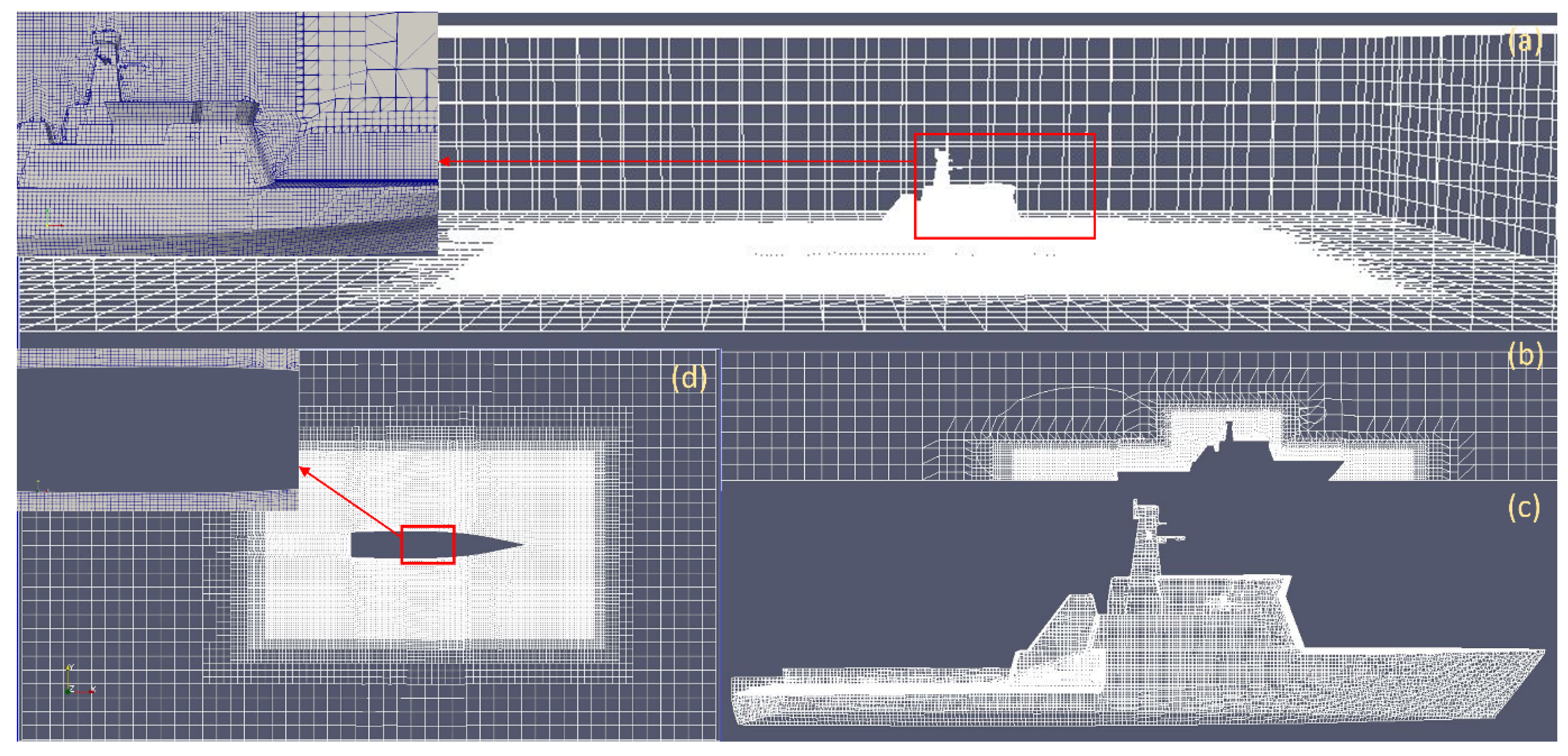
2.2. Mesh
2.3. The Solver and Computational Resource
3. Results
- 1.
- Turbulence model dependency study for a mesh with 3.95 million cells using three different approaches, by modelling with SST K-Omega and K-Epsilon two-equation turbulence models, and by resolving with the Delayed Detached Eddy Simulation.
- 2.
- Time convergence study for three inflow angles (0°, 45°, 90°, 135°, and 180°) using a mesh with 3.95 Mcells and the selected (SST K-Omega) turbulence model.
- 3.
- Grid and time step dependency study for a 45° inflow angle using three mesh resolutions and the selected turbulence model.
- 4.
- Study of aerodynamic forces and moments encountered by the vessel while facing wind from different inflow angles. In total, the resulting database includes wind loads for 24 inflow angles ranging from head to stern flow.
- 5.
- Study of scale effects on aerodynamic load prediction by simulating five selected cases in full-scale and comparing with model scale results.
3.1. Preliminary Studies
3.1.1. Turbulence Models
3.1.2. Time Domain Settling
3.1.3. Grid Convergence Study
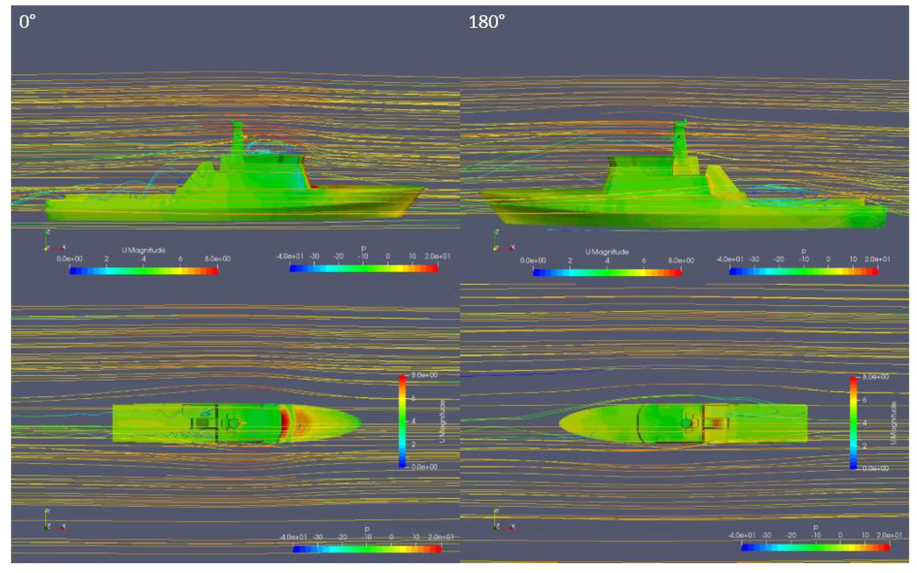
3.2. Flow Field Visualization Results
3.3. Force and Moment Results
3.4. Comparison of Results with Blendermann Models
4. Conclusions
Author Contributions
Funding
Institutional Review Board Statement
Informed Consent Statement
Data Availability Statement
Conflicts of Interest
References
- Sutulo, S.; Moreira, L.; Guedes Soares, C. Mathematical Models for Ship Path Prediction in Manoeuvring Simulation Systems. Ocean. Eng. 2002, 29, 1–19. [Google Scholar] [CrossRef]
- Sutulo, S.; Guedes Soares, C. Mathematical models for simulation of manoeuvring performance of ships. In Marine Technology and Engineering; Guedes Soares, C., Garbatov, Y., Fonseca, N., Teixeira, A.P., Eds.; Taylor & Francis Group: London, UK, 2011; pp. 661–698. [Google Scholar]
- Guedes Soares, C.; Sutulo, S.; Francisco, R.A.; Santos, F.M.; Moreira, L. Full-Scale Measurements of the Manoeuvring Capabilities of a Catamaran. In Proceedings of the International Conference on Hydrodynamics of High Speed Craft, London, UK, 24–25 November 1999; Royal Institution of Naval Architects: London, UK, 1999; pp. 1–12. [Google Scholar]
- Guedes Soares, C.; Francisco, R.A.; Moreira, L.; Laranjinha, M. Full-Scale Measurements of the Manoeuvering Capabilities of Fast Patrol Vessels, Argos Class. Mar. Technol. 2004, 41, 7–16. [Google Scholar]
- Sutulo, S.; Guedes Soares, C. An Algorithm for Offline Identification of Ship Manoeuvring Mathematical Models after Free-Running Tests. Ocean. Eng. 2014, 79, 10–25. [Google Scholar] [CrossRef]
- Wang, Z.; Guedes Soares, C.; Zou, Z.J. Optimal design of excitation signal for identification of nonlinear ship manoeuvring model. Ocean. Eng. 2020, 196, 106778. [Google Scholar] [CrossRef]
- Dubbioso, D.; Viviani, M. Aspects of twin screw ships semi-empirical maneuvering models. Ocean. Eng. 2012, 48, 69–80. [Google Scholar] [CrossRef]
- Sutulo, S.; Guedes Soares, C. On the application of empiric methods for prediction of ship manoeuvring properties and associated uncertainties. Ocean. Eng. 2019, 186, 106111. [Google Scholar] [CrossRef]
- Vettor, R.; Prpić-Oršić, J.; Guedes Soares, C. The effect of wind loads on the attainable ship speed on seaways. In Towards Green Marine Technology and Transport; Guedes Soares, C., Dejhalla, R., Pavletic, D., Eds.; Taylor and Francis: London, UK, 2015. [Google Scholar]
- Vettor, R.; Prpić-Oršić, J.; Guedes Soares, C. Impact of wind loads on long-term fuel consumption and emissions in trans-oceanic shipping. Brodogradnja 2018, 69, 15–28. [Google Scholar] [CrossRef]
- Moreira, L.; Vettor, R.; Guedes Soares, C. Neural network approach for predicting ship speed and fuel consumption. J. Mar. Sci. Eng. 2021, 9, 119. [Google Scholar] [CrossRef]
- Owens, R.; Palo, P. Wind-Induced Steady Loads on Ships; Technical Note; Naval Civil Engineering Laboratory: Port Hueneme, CA, USA, 1982; p. 93043. [Google Scholar]
- Blendermann, W. Wind Loadings of Ships—Collected Data from Wind Tunnel Tests in Uniform Flow; Report 574; Institute of Naval Architecture: London, UK, 1996. [Google Scholar]
- Blendermann, W. Practical Ship and Offshore Structure Aerodynamics; Technische Universität Hamburg-Harburg: Hamburg, Germany, 2013. [Google Scholar]
- Andersen, I.M.V. Wind Loads on post-Panamax container ship. Ocean. Eng. 2013, 58, 115–134. [Google Scholar] [CrossRef]
- Haddara, M.; Guedes Soares, C. Wind Loads on Marine Structures. Mar. Struct. 1999, 12, 199–210. [Google Scholar] [CrossRef]
- Hassan, K.; White, M.F.; Ciortan, C. Effect of Container Stack Arrangement on the Power Optimization of a Container Ship. J. Ship Prod. Des. 2012, 28, 10–19. [Google Scholar] [CrossRef]
- Koop, A.; Rossin, B.; Guilherme, V. Predicting wind loads on typical offshore vessels using CFD. In Proceedings of the ASME 31th International Conference on Ocean, Offshore and Arctic Engineering (OMAE2012), Rio de Janeiro, Brazil, 1–7 July 2012. [Google Scholar]
- Luquet, R.; Vonier, P.; Prior, A.; Leguen, J.F. Aerodynamic Loads on a Heeled Ship. In Proceedings of the 12th International Conference on the Stability of Ship and Ocean Vehicles, Glasgow, UK, 14–19 June 2015. [Google Scholar]
- Wnȩk, A.D.; Guedes Soares, C. CFD assessment of the wind load on an LNG carrier and floating platform models. Ocean. Eng. 2015, 97, 30–36. [Google Scholar] [CrossRef]
- Wnȩk, A.D.; Paço, A.; Zhou, X.Q.; Sutulo, S.; Guedes Soares, C. Experimental Study of Aerodynamic Loads on an LNG Carrier and Floating Platform. Appl. Ocean. Res. 2015, 51, 309–319. [Google Scholar] [CrossRef]
- Watanabe, I.; Nguyen, T.V.; Miyake, S.; Shimizu, N.; Ikeda, Y. A Study on Reduction of Air Resistance Acting on A Large Container Ship. In Proceedings of the 8th Asia-Pacific Workshop on Marine Hydrodynamics in Naval Architecture, Ocean Technology and Constructions, Hanoi, Vietnam, 20–23 September 2016. [Google Scholar]
- Nguyen, T.V.; Kinugawa, A.; Shimizu, N.; Ikeda, Y. Studies on Air Resistance Reduction Methods for a Large Container Ship (Part 1). In Proceedings of the Japan Society of Naval Architects and Ocean Engineers, Autumn Meeting, Okayama, Japan, 21–22 November 2016. [Google Scholar]
- Majidian, H.; Azarsina, F. Aerodynamic Simulation of a Containership to Evaluate Cargo Configuration Effect on Frontal Wind Loads. China Ocean. Eng. 2018, 32, 196–205. [Google Scholar] [CrossRef]
- Majidian, H.; Azarsina, F. Numerical simulation of container ship in oblique winds to develop a wind resistance model based on statistical data. J. Int. Marit. Saf. Environ. Aff. Shipp. 2018, 2, 67–88. [Google Scholar] [CrossRef]
- Wang, P.; Wang, F.; Chen, Z. Investigation on aerodynamic performance of luxury cruise ship. Ocean. Eng. 2020, 213, 107790. [Google Scholar] [CrossRef]
- Forrest, J.; Owen, I. An investigation of ship airwakes using Detached-Eddy simulation. Comput. Fluids 2010, 39, 656–673. [Google Scholar] [CrossRef]
- Thornber, B.; Starr, M.; Drikakis, D. Implicit large eddy simulation of ship airwakes. Aeronaut. J. 2010, 114, 715–736. [Google Scholar] [CrossRef] [Green Version]
- Forrest, J.S.; Kääriä, C.; Owen, I. Evaluating ship superstructure aerodynamics for maritime helicopter operations through CFD and flight simulation. Aeronaut. J. 2016, 120, 1578–1603. [Google Scholar] [CrossRef]
- Yuan, W.; Wall, A.; Lee, R. Combined numerical and experimental simulations of unsteady ship airwakes. Comput. Fluids 2018, 172, 29–53. [Google Scholar] [CrossRef]
- Thedin, R.; Kinzel, M.; Horn, J.; Schmitz, S. Coupled simulations of atmospheric turbulence-modified ship airwakes and helicopter flight dynamics. J. Aircr. 2019, 56, 812–824. [Google Scholar] [CrossRef]
- Watson, N.A.; Kelly, M.F.; Owen, I.; Hodge, S.J.; White, M.D. Computational and experimental modelling study of the unsteady airflow over the aircraft carrier HMS Queen Elizabeth. Ocean Eng. 2019, 172, 562–574. [Google Scholar] [CrossRef]
- Linton, D.; Thornber, B. Quantifying uncertainty in turbulence resolving ship airwake simulations. Ocean. Eng. 2021, 229, 108983. [Google Scholar] [CrossRef]
- Flyvefisken-Class Patrol Vessel. 2021. Available online: https://en.wikipedia.org/wiki/Flyvefisken-class_patrol_vessel (accessed on 15 August 2021).
- Flyvefisken Class (SF 300). Available online: https://www.naval-technology.com/projects/fly/ (accessed on 15 August 2021).
- ITTC-7.5-03-02-03; ITTC-2011—Recommended Procedures and Guidelines. Practical Guidelines for Ship CFD and Application. Curran Associates, Inc.: Red Hook, NY, USA, 2012.
- Labanti, J.; Islam, H.; Guedes Soares, C. CFD assessment of Ropax hull resistance with various initial drafts and trim angles. In Maritime Technology and Engineering 3; Guedes Soares, C., Santos, T.A., Eds.; Taylor & Francis Group: London, UK, 2016; pp. 325–332. [Google Scholar]
- Weller, H.G.; Tabor, G.; Jasak, H.; Fureby, C. A tensorial approach to computational continuum mechanics using object-oriented techniques. Comput. Phys. 1998, 12, 620–631. [Google Scholar] [CrossRef]
- Frisch, U. Turbulence: The Legacy of A.N. Kolmogorov, 1st ed.; Cambridge University Press: Cambridge, UK, 1995. [Google Scholar]
- Menter, F.R. Zonal Two Equation k-ω Turbulence Models for Aerodynamic Flows. In Proceedings of the 23rd Fluid Dynamics, Plasma Dynamics, and Lasers Conference, Orlando, FL, USA, 6–9 July 1993; AIAA Paper: Reston, VA, USA, 1993; p. 2906. [Google Scholar]
- Launder, B.E.; Spalding, D.B. The numerical computation of turbulent flows. Comput. Methods Appl. Mech. Eng. 1974, 3, 269–289. [Google Scholar] [CrossRef]
- Wilcox, C.D. Turbulence Modeling for CFD, 2nd ed.; DCW Industries: La Canada, CA, USA, 1998. [Google Scholar]
- Gritskevich, M.S.; Garbaruk, A.V.; Schütze, J.; Menter, F.R. Development of DDES and IDDES Formulations for the k-w Shear Stress Transport Model. Flow Turbul. Combust. 2012, 88, 431–449. [Google Scholar] [CrossRef]
- ITTC-7.5-03-01-01; ITTC-2008—Recommended Procedures and Guidelines. Uncertainty Analysis in CFD Verification and Validation Methodology and Procedures. Curran Associates, Inc.: Red Hook, NY, USA, 2009.
- Celik, I.B.; Ghia, U.; Roache, P.J.; Freitas, C.J.; Coleman, H.; Raad, P.E. Procedure for Estimation and Reporting of Uncertainty Due to Discretization in CFD Applications. J. Fluids Eng. Trans. ASME 2008, 130, 078001. [Google Scholar]
- Islam, H.; Guedes Soares, C. Uncertainty analysis in ship resistance prediction using OpenFOAM. Ocean. Eng. 2019, 191, 105805. [Google Scholar] [CrossRef]
- Islam, H.; Guedes Soares, C. Assessment of uncertainty in the CFD simulation of the wave-induced loads on a vertical cylinder. Mar. Struct. 2021, 80, 103088. [Google Scholar] [CrossRef]
- Wang, S.; Islam, H.; Guedes Soares, C. Uncertainty due to discretization on the ALE algorithm for predicting water slamming loads. Mar. Struct. 2021, 80, 103086. [Google Scholar] [CrossRef]
- Islam, H.; Guedes Soares, C.; Liu, J.; Wang, X. Propulsion power prediction for an inland container vessel in open and restricted channel from model and full-scale simulations. Ocean. Eng. 2021, 229, 108621. [Google Scholar] [CrossRef]


| Drift Angle (Deg) | Turbulence Model | ||||
|---|---|---|---|---|---|
| 45 | SST K-Omega | −0.22 | 0.85 | −0.522 | 0.16 |
| K-Epsilon | −0.19 | 0.85 | −0.515 | 0.16 | |
| DDES | −0.13 | 0.92 | −0.564 | 0.17 | |
| 90 | SST K-Omega | −0.04 | 1.10 | −0.599 | 0.06 |
| K-Epsilon | 0.03 | 1.14 | −0.587 | 0.06 | |
| DDES | −0.12 | 1.17 | −0.627 | 0.06 | |
| 135 | SST K-Omega | 0.36 | 0.93 | −0.458 | −0.06 |
| K-Epsilon | 0.29 | 1.00 | −0.484 | −0.08 | |
| DDES | 0.29 | 0.98 | −0.471 | −0.06 |
| Mesh | Total Number of Cells | Dimensions x (m) | Of y (m) | Cells | Minimum Layer Thickness | Non-Dimensional Wall Distance, y+ | Coarsening Ratio |
|---|---|---|---|---|---|---|---|
| 1 | 0.01953 | 0.01875 | 0.01875 | 0.00375 | 65 | 1.00 | |
| 2 | 0.02500 | 0.02500 | 0.02344 | 0.00500 | 87 | 1.30 | |
| 3 | 0.03125 | 0.03125 | 0.03125 | 0.00625 | 108 | 1.25 |
| Property | |||||
|---|---|---|---|---|---|
| Simulation results | (fine) | −3.73 | 50.18 | −16.45 | 53.25 |
| (mid) | −3.65 | 49.95 | −16.68 | 50.20 | |
| (coarse) | −4.63 | 49.84 | −16.47 | 48.48 | |
| Refinement ratio | 1.3 | 1.3 | 1.3 | 1.3 | |
| r32 = h3/h2 | 1.25 | 1.25 | 1.25 | 1.25 | |
| Difference of estimation | 0.0778 | −0.233 | −0.233 | −3.050 | |
| −0.985 | −0.114 | 0.208 | −1.720 | ||
| Convergence | −0.079 | 2.050 | −1.122 | 1.773 | |
| Order of accuracy | 11.25 | 1.96 | 0.41 | 1.45 | |
| Extrapolated values | −3.73 | 50.53 | −14.39 | 59.84 | |
| −3.56 | 50.16 | −18.85 | 54.70 | ||
| Approximate relative error | −0.0209 | −0.0046 | 0.0142 | −0.0573 | |
| 0.270 | −0.0023 | −0.0125 | −0.0343 | ||
| Extrapolated relative error | −0.00115 | −0.0069 | 0.1428 | −0.1101 | |
| 0.0245 | −0.0041 | −0.1151 | −0.0823 | ||
| Grid convergence index (GCI) | GCI21 | −0.0014 | −0.0086 | 0.15616 | −0.15467 |
| GCI32 | 0.0298 | −0.0052 | −0.1626 | −0.1121 | |
| Corrected uncertainty | 0.0288% | 0.1729% | 3.1231% | 3.0933% | |
| 0.5968% | 0.1039% | 3.2522% | 2.2421% |
| Drift Angle | ||||||||
|---|---|---|---|---|---|---|---|---|
| 0 | −7.90 | 0.17 | −0.07 | 1.00 | −0.48 | 0.00 | −0.002 | 0.00 |
| 10 | −9.19 | 9.33 | −2.39 | 15.94 | −0.56 | 0.16 | −0.075 | 0.05 |
| 20 | −8.68 | 24.02 | −7.49 | 29.93 | −0.53 | 0.41 | −0.234 | 0.09 |
| 30 | −6.75 | 39.57 | −12.41 | 43.33 | −0.41 | 0.68 | −0.388 | 0.14 |
| 40 | −4.71 | 45.88 | −15.05 | 51.10 | −0.29 | 0.78 | −0.471 | 0.16 |
| 45 | −3.65 | 49.95 | −16.70 | 50.20 | −0.22 | 0.85 | −0.522 | 0.16 |
| 50 | −2.82 | 52.97 | −17.44 | 49.76 | −0.17 | 0.90 | −0.545 | 0.16 |
| 60 | −3.71 | 56.42 | −16.75 | 43.31 | −0.23 | 0.96 | −0.524 | 0.14 |
| 70 | −3.38 | 62.12 | −17.53 | 37.22 | −0.21 | 1.06 | −0.548 | 0.12 |
| 80 | −3.15 | 66.06 | −19.85 | 27.79 | −0.19 | 1.13 | −0.621 | 0.09 |
| 85 | 0.22 | 63.21 | −19.62 | 20.00 | 0.01 | 1.08 | −0.614 | 0.06 |
| 90 | −0.62 | 64.51 | −19.15 | 18.41 | −0.04 | 1.10 | −0.599 | 0.06 |
| 95 | −2.40 | 66.04 | −19.21 | 7.71 | −0.15 | 1.13 | −0.601 | 0.02 |
| 100 | −2.15 | 64.86 | −20.09 | 4.56 | −0.13 | 1.11 | −0.628 | 0.01 |
| 110 | 0.63 | 63.21 | −17.03 | −9.72 | 0.04 | 1.08 | −0.533 | −0.03 |
| 120 | 2.19 | 62.15 | −16.69 | −10.20 | 0.13 | 1.06 | −0.522 | −0.03 |
| 130 | 5.00 | 55.55 | −15.20 | −15.32 | 0.30 | 0.95 | −0.475 | −0.05 |
| 135 | 5.89 | 54.58 | −14.66 | −18.81 | 0.36 | 0.93 | −0.458 | −0.06 |
| 140 | 6.37 | 51.20 | −13.93 | −21.91 | 0.39 | 0.87 | −0.436 | −0.07 |
| 145 | 7.70 | 46.99 | −12.60 | −22.67 | 0.47 | 0.80 | −0.394 | −0.07 |
| 150 | 7.73 | 41.70 | −11.20 | −21.95 | 0.47 | 0.71 | −0.350 | −0.07 |
| 160 | 8.83 | 28.57 | −6.99 | −14.12 | 0.54 | 0.49 | −0.219 | −0.04 |
| 170 | 9.97 | 13.03 | −2.80 | −7.38 | 0.61 | 0.22 | −0.087 | −0.02 |
| 180 | 8.25 | 0.20 | −0.02 | −0.27 | 0.50 | 0.00 | −0.001 | 0.00 |
| Drift Angle | NA (N-m) | |||||||
|---|---|---|---|---|---|---|---|---|
| 0 | −7396.12 | −174.56 | 700.00 | −1227 | −0.44 | 0.00 | 0.00 | 0.00 |
| 45 | −4201.27 | 48,412.00 | −210,030.51 | 535,125 | −0.25 | 0.82 | −0.65 | 0.17 |
| 90 | −1338.89 | 64,698.98 | −251,004.00 | 135,944 | −0.08 | 1.10 | −0.78 | 0.04 |
| 135 | 5146.32 | 57,890.83 | −221,197.14 | −264,855 | 0.31 | 0.98 | −0.69 | −0.08 |
| 180 | 9579.00 | −272.46 | 1490.47 | −2939.8 | 0.58 | 0.00 | 0.00 | 0.00 |
Publisher’s Note: MDPI stays neutral with regard to jurisdictional claims in published maps and institutional affiliations. |
© 2022 by the authors. Licensee MDPI, Basel, Switzerland. This article is an open access article distributed under the terms and conditions of the Creative Commons Attribution (CC BY) license (https://creativecommons.org/licenses/by/4.0/).
Share and Cite
Islam, H.; Sutulo, S.; Guedes Soares, C. Aerodynamic Load Prediction on a Patrol Vessel Using Computational Fluid Dynamics. J. Mar. Sci. Eng. 2022, 10, 935. https://doi.org/10.3390/jmse10070935
Islam H, Sutulo S, Guedes Soares C. Aerodynamic Load Prediction on a Patrol Vessel Using Computational Fluid Dynamics. Journal of Marine Science and Engineering. 2022; 10(7):935. https://doi.org/10.3390/jmse10070935
Chicago/Turabian StyleIslam, Hafizul, Serge Sutulo, and C. Guedes Soares. 2022. "Aerodynamic Load Prediction on a Patrol Vessel Using Computational Fluid Dynamics" Journal of Marine Science and Engineering 10, no. 7: 935. https://doi.org/10.3390/jmse10070935