Fast Finite-Time Path-Following Control of Unmanned Surface Vehicles with Sideslip Compensation and Time-Varying Disturbances

Abstract

This paper studies the fast finite-time path following of underactuated unmanned surface vehicles (USV) with sideslip compensation, time-varying disturbances and input saturation. In the guidance module, the fast finite-time predictor-based line-of-sight (FFTPLOS) is proposed to overcome the large guidance angle and high-frequency oscillation and eliminate the sideslip angle with finite time. Then, the robust finite-time feedback control is applied to keep the vehicle following the desired path in the control module, where the reduced-order extended state observers (ROESO) are applied to deal with time-varying disturbances. Additionally, fast finite-time auxiliary dynamic systems with smoothly switching functions (FFTADS-SSF) achieve the saturation constraints on actuators with low consumption. The stability analysis proves that the guidance-control system of USVs is uniformly ultimately bounded stable within finite time. The effectiveness and performance of this proposed scheme are superior to the comparison schemes.

1. Introduction

More attention has been paid to the academic research on unmanned surface vehicles (USV) over the past several years because of its widespread applications in civilian fields such as casualty rescue, target search and reconnaissance missions of the military [1,2]. Path following is an indispensable branch of the motion control of unmanned systems, including unmanned surface vehicle (USV) systems [3], unmanned aerial vehicle (UAV) systems [4] and unmanned ground vehicle (UGV) systems [5]. It is known that the control objective of path following is to track the geometric path on the plane without time constraints. Therefore, path following has played an indispensable role in its brilliant properties such as dynamic path planning and practical engineering applications [6,7]. By incorporating guidance methods into path following [8], the control design of USVs can achieve the convergence of path-following error and obtain better transient tracking performance, improving the safety of USV maneuvering.

Numerous academic studies have been published on the path-following control of USVs [3,6,7], mainly involving the research guidance module in kinematics and control module in dynamics. At the kinematics level of USV, the line-of-sight (LOS) method is a common technique within the guidance system due to the merits of simplicity, efficiency, and ease of implementation. The traditional LOS guidance law has proposed to obtain the reference heading angle by the position tracking errors and look-ahead distance. Since most USVs have no thrust in the cross-track direction, a small sway velocity is generated by the environmental disturbances, resulting in a small sideslip angle. Although it is small, it also affects the accuracy of path following. Therefore, how to remove its influence becomes challenging research. The integral LOS guidance strategy is an established controller, which effectively compensates for drift forces and offsets the sideslip angle [9]. Meanwhile, an adaptive LOS guidance principle used by both integral term and adaptive method is established to handle constant or slow time-varying sideslip angles [10]. Additionally, a novel LOS guidance law with reduced-order ESO is employed to solve the sideslip angle [11]. During transient state, large tracking errors may make the guidance heading deviate from the desired angle in the mentioned studies. In [12,13], a practical proportional sliding-mode controller is applied to deal with the problem of trajectory tracking of the USV. In this paper, an improved predictor-based LOS guidance method with fast finite time not only provides simplicity and interpretation but also addresses the smoothing and fast identification of time-varying sideslip angle and is used to compensate for the vehicle sideslip due to environmental impacts.

In addition to the guidance module, the control module should be considered to design the whole path-following system, which makes the vehicle velocity and attitude fulfill the requirements of LOS guidance. Then, much theoretical research, including the fuzzy control [14], backstepping method [15], active disturbance rejection control [16], trajectory linearization control [17] and sliding-mode control [18], has been applied to control systems. By designing a virtual control law, the linearization of the USV model is avoided, and the global asymptotic stability of the system is proved [19]. Adaptive PI sliding-mode control is applied to deal with the path-following problem of USVs under unknown model parameters and environmental disturbances. The advantage of this method is that there is no need to assume that the upper bound of the disturbance is known [20]. An adaptive integral sliding-mode path-following controller is developed via RBF neural network to improve the robustness [21]. However, in [22,23], a nonlinear disturbance observer (NDO) is summarized to solve parameter uncertainty and external disturbance. Although the above research methods are all designed controllers by sliding-mode control, they bring tremors to the system. This phenomenon can weaken but cannot eliminate.

In engineering applications, input saturation is unavoidable because of the physical restrictions of the actuator, while most research [13,14,15,16,18,19,20] ignored this. Therefore, predefined physical limitations are introduced to control the actuator within a reasonable working range, which leads to instability of the entire system [24]. To solve the above problems, on the one hand, other antisaturation methods are proposed in [25,26,27], which are employed to handle the input saturation. In [25], the Gauss error function is applied to approximate the uncertainties of the input saturation, which is described by the control inputs with the bounded multiplicative gains in [26]. Meanwhile, the MPC controller with input constraints is proposed that can be easily adjusted to produce outputs that are not saturated in [27]. On the other hand, an auxiliary system is proposed in [17,28] to deal with the input saturation. A robust nonlinear controller is developed to the dynamic positioning (DP) system for vehicles, which solves input saturation by the auxiliary dynamic system (ADS) in [29]. In [30], a novel auxiliary dynamic system is applied to address actuator saturation, and the finite-time auxiliary dynamic system is developed to solve the saturation problem in [31]. According to the above research, this paper adopts the improved finite-time auxiliary dynamic system with smoothly switching function (FFTADS-SFF) that limits the input within the reasonable range, reducing input energy consumption, thereby improving the tracking and control performance.

Inspired by the above results, this paper studies the path following of underactuated USVs with sideslip compensation, time-vary disturbances and input saturation and proposes a fast finite-time control strategy via FFTPLOS guidance, ROESOs and FFTADS-SSF. The main contributions of the proposed control scheme are summarized as follows:

(1)

In the guidance module, compared with the PLOS [12,13] that prediction errors are applied to in order to identify the sideslip angle, the FFTPLOS is employed instead of the PLOS such that this angle is compensated within a finite time. The better estimated performances, not only in steady state but also in transient state, are reached rapidly without causing high-frequency oscillation.

(2)

In the control module, a robust finite-time feedback control law is applied to keep vehicles following the desired path. Moreover, the ROESO provide accuracy for the time-varying disturbances on the along velocity and cross velocity, achieving a prominent control effect at the USV’s kinetic level under complex ocean conditions. More importantly, the system exhibits better disturbance estimation performance than [22].

(3)

Compared with the ADS in [28] that alleviates input saturation of the propulsion systems, the novel FFTADS-SSF is introduced to replace the ADS such that actuator input is limited within a finite settling time, which produces lower consumption. The better physical constraints are superior to the ADS scheme in tracking performance and control accuracy.

The other sections of this paper are arranged as follows. Section 2 introduces the problem formulation and preliminaries. Section 3 presents the design details of the FFTPLOS guidance law. Section 4 introduces the design of the path-tracking controller with the ROESO. Section 5 describes a proof-of-system stability. Section 6 provides simulations of path following under time-varying disturbances. Finally, the conclusion of this paper is in Section 7.

2. Problem Formulation and Preliminaries

This section mainly describes the 3-DOF USV model, position error dynamic equation, lemmas and assumptions and control objectives.

2.1. USV Model

Ignoring the heave and pitching movements of USVs, the path variables are illustrated in Figure 1, where $P={[x,y]}^T$ and $P_d={\left[x\left(\theta \right),y\left(\theta \right)\right]}^T$ represent the current location and the arbitrary location of the predefined path, respectively. Considering the influence of the unknown time-varying disturbances such as ocean current, we establish a 3-DOF kinematic model of the underactuated USV [21,32].

$$\left\{\begin{array}{c}\dot{\mathit{\eta }}=\mathit{J}\left(\psi \right)v\hfill \\ \mathit{M}\dot{v}=-\mathit{C}\left(v\right)v-\mathit{D}v+\mathbf{\tau }\hfill \end{array}\right.$$

(1)

where $\mathit{\eta }={[x,y,\psi ]}^T$ is the position and heading in the earth-fixed frame, and $\psi \in \left[0,2\pi \right]$. $v={\left[u,v,r\right]}^T$ is the surge, sway and yaw velocities in the body-fixed frame. $\mathbf{\tau }={[{\tau }_u,0,{\tau }_r]}^T$ is the control force and moment. $\mathit{M}$ is the USV inertia matrix, $\mathit{C}$ and $\mathit{D}$ are the USV’s Coriolis–centripetal, linear and nonlinear damping matrices, respectively. Their specific expressions are given as follows

$$\begin{array}{ccc}& \mathit{M}=\left[\begin{array}{cccc}& m_{11}\hfill & \hfill 0& 0\hfill \\ & 0\hfill & \hfill m_{22}& m_{23}\hfill \\ & 0\hfill & \hfill m_{32}& m_{33}\hfill \end{array}\right]\hfill & \hfill \mathit{C}=\left[\begin{array}{cccc}& 0\hfill & \hfill 0& c_{13}\hfill \\ & 0\hfill & \hfill 0& c_{23}\hfill \\ & c_{31}\hfill & \hfill c_{32}& 0\hfill \end{array}\right]\\ & \mathbf{D}=\left[\begin{array}{cccc}& d_{11}\hfill & \hfill 0& 0\hfill \\ & 0\hfill & \hfill d_{22}& d_{23}\hfill \\ & 0\hfill & \hfill d_{32}& d_{33}\hfill \end{array}\right]\hfill & \hfill \mathit{J}\left(\psi \right)=\left[\begin{array}{cccc}& cos\psi \hfill & \hfill -sin\psi & 0\hfill \\ & sin\psi \hfill & \hfill cos\psi & 0\hfill \\ & 0\hfill & \hfill 0& 1\hfill \end{array}\right]\end{array}$$

where $m_{11}$, $m_{22}$, $m_{33}$, $m_{23}$ and $m_{32}$ denote the USV inertia mass, including added mass. The terms $d_{11}$, $d_{22}$, $d_{33}$, $d_{23}$ and $d_{32}$ are hydrodynamic derivatives, including the linear and nonlinear damping terms. The rotational matrix $\mathit{J}$ is a transformation between the body-fixed and earth-fixed frame. The Coriolis–centripetal terms meet $c_{13}=-c_{31}=m_{22}v-0.5(m_{23}+m_{32})r$, $c_{23}=-c_{32}=m_{11}u$, and $m_{23}=m_{32}$ [32].

Remark 1.

There are off-diagonal terms $m_{23}$ and $m_{32}$ in the inertia matrix $\mathit{M}$ which are not equal to 0 and satisfy $m_{23}$ = $m_{32}$. The reason for the above is that the profile of the bow is different from that of the stern [33]. In this case, the resulting yaw moment ${\tau }_r$ acts directly on the roll and yaw dynamics of the USV simultaneously.

To solve the above problem, the following coordinate transformation [34] is adopted, $\overline{x}=x+\epsilon$ cos $\psi$, $\overline{y}=y+\epsilon$ sin $\psi$, $\overline{u}=u,\overline{v}=v+\epsilon r$ and $\overline{r}=r$, where $ϵ=m_{23}/m_{22}>0$, for nonzero off-diagonal terms. Through coordinate transformation, the inertial matrix of the USV is transformed into an “oblique symmetry form”, so that the rocking dynamics of the USV can get rid of the moment ${\tau }_r$. Generating a new USV output variable ($\overline{x}$, $\overline{y}$, $\psi$) to replace the original (x, y, $\psi$), one yields

$$\left\{\begin{array}{c}\dot{\overline{x}}=\overline{u}cos\psi -\overline{v}sin\psi \hfill \\ \dot{\overline{y}}=\overline{u}sin\psi +\overline{v}cos\psi \hfill \\ \dot{\psi }=\overline{r}\hfill \end{array}\right.\left\{\begin{array}{c}\dot{\overline{u}}=F_u\left(\overline{u},\overline{v},\overline{r}\right)+{\tau }_u+d_u\hfill \\ \dot{\overline{v}}=X\left(\overline{u}\right)\overline{r}+Y\left(\overline{u}\right)\overline{v}+d_v\hfill \\ \dot{\overline{r}}=F_r\left(\overline{u},\overline{v},\overline{r}\right)+{\tau }_r+d_r\hfill \end{array}\right.$$

(2)

where $F_u\left(\overline{u},\overline{v},\overline{r}\right)=\frac{m_{22}}{m_{11}}\overline{v}\overline{r}-\frac{d_{11}}{m_{11}}\overline{u}$, $Y\left(\overline{u}\right)=-\frac{1}{m_{22}}{d}_{22}$, $X\left(\overline{u}\right)=\frac{m_{11}+\epsilon d_{22}-d_{23}}{m_{22}}$, $F_r\left(\overline{u},\overline{v},\overline{r}\right)=\frac{(m_{11}{m}_{22}-m_{{}_{22}}^2)\overline{u}+(m_{23}{d}_{22}-m_{22}{d}_{32})}{m_{22}{m}_{33}-m_{23}^2}\overline{v}+\frac{m_{23}{d}_{23}-m_{22}{d}_{33}+m_{23}{d}_{32}-\epsilon m_{23}{d}_{22}}{m_{22}{m}_{33}-m_{23}^2}\overline{r}$. $X\left(\overline{u}\right)$ and $Y\left(\overline{u}\right)$ are linear functions of velocity and are also continuously passively bounded. $\mathit{d}={\left[d_u,d_v,d_r\right]}^T$ denotes the unknown time-varying environmental disturbances.

Remark 2.

Move the origin of the attached coordinate system to a positive distance ε from the center of gravity, so that the USV system (1) is transformed into a diagonal form (2). If $(\overline{x},\overline{y})$ instead of $(x,y)$ is regarded as the USV position, the above-mentioned method is used to re-select $\mathit{\eta }={[x,y,\psi ]}^T$, $v={\left[u,v,r\right]}^T$ and $\mathbf{\tau }={[{\tau }_u,0,{\tau }_r]}^T$ as the position vector, velocity vector and surge force and yaw moment of the mathematical model of the USV motion after coordinate transformation.

Considering the physical constraints [35], the control inputs with nonlinear saturations are described as follows

$${\tau }_i=\left\{\begin{array}{cc}\hfill {\tau }_{imax},& {\tau }_{i0}>{\tau }_{imax}\hfill \\ \hfill {\tau }_{i0},& {\tau }_{imin}\le {\tau }_{i0}\le {\tau }_{imax}\hfill \\ \hfill {\tau }_{imin},& {\tau }_{i0}<{\tau }_{imin}\hfill \end{array}\right.$$

(3)

where ${\tau }_{imin}$ and ${\tau }_{imax}(i=u,r)$ are the minimum and maximum control inputs generated by the actuators, according to physical constraints of the motor’s rotational speed and rudder deflection. ${\tau }_{i0}(i=u,r)$ is the command control input of the proposed controller, which needs to be designed.

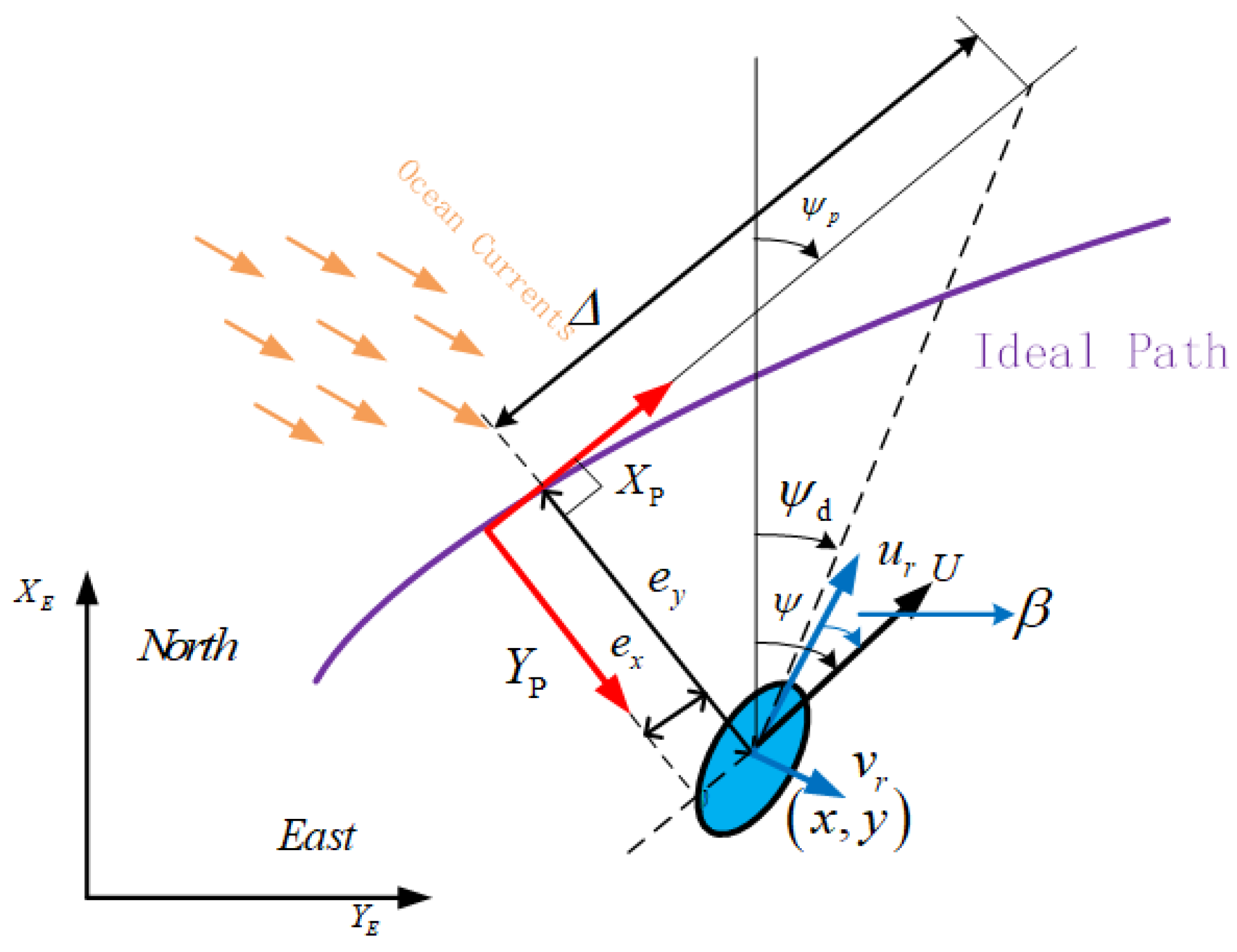
2.2. Position Error Dynamic Equation

Since the path-following control of USVs does not have time constraints, we need to define the ideal parameterized path $P_d(x_d\left(\theta \right),y_d\left(\theta \right))$. Additionally, the tangential angle ${\alpha }_k$ of the path curve is as follows:

$${\alpha }_k\left(\theta \right)=arctan(\dot{y_d}\left(\theta \right),\dot{x_d}\left(\theta \right))$$

(4)

where ${\dot{x}}_d=\partial x_d/\phantom{\partial x_d\partial }\partial \theta$ and ${\dot{y}}_d=\partial y_d/\phantom{\partial y_d\partial }\partial \theta$.

As shown in Figure 1, for the USV located at $P_d(x_d\left(\theta \right),y_d\left(\theta \right))$, its position tracking error of along-track $x_e$ and cross-track $y_e$ relative to the ideal position $(x,y)$ is described in the path-tangential reference frame.

$$\left[\begin{array}{c}{x}_e\\ y_e\end{array}\right]={\left[\begin{array}{cc}cos{\alpha }_k& -sin{\alpha }_k\\ sin{\alpha }_k& cos{\alpha }_k\end{array}\right]}^T\left[\begin{array}{c}x-x_d\left(\theta \right)\\ y-y_d\left(\theta \right)\end{array}\right]$$

(5)

Taking the time derivative of the along-track error $x_e$ in (5) yields

$$\begin{array}{c} {\dot{x}}_e=\dot{x}cos{\alpha }_k+\dot{y}sin{\alpha }_k-{\dot{x}}_d\left(\theta \right)cos{\alpha }_k-{\dot{y}}_d\left(\theta \right)sin{\alpha }_k\\ +{\dot{\alpha }}_k[-(x-x_d\left(\theta \right))sin{\alpha }_k+(y-y_d\left(\theta \right)cos{\alpha }_k]\end{array}.$$

(6)

Inserting (5) into (6), it follows that

$${\dot{x}}_e=Ucos(\psi -{\alpha }_k)cos\beta -Usin(\psi -{\alpha }_k)sin\beta +{\dot{\alpha }}_k{y}_e-u_p$$

(7)

In (7), the velocity $u_p$ of the virtual reference point is regarded as the control input to control the convergence of the along-track error $x_e$

$$u_p=\dot{\theta }\sqrt{{\dot{x}}_d^2\left(\theta \right)+{\dot{y}}_d^2\left(\theta \right)}$$

(8)

Similarly, taking the time derivative of the cross-track error $y_e$ in (5) yields

$$\begin{array}{c} {\dot{y}}_e=-\dot{x}sin{\alpha }_k+\dot{y}cos{\alpha }_k+{\dot{x}}_d\left(\theta \right)sin{\alpha }_k-{\dot{y}}_d\left(\theta \right)cos{\alpha }_k\\ -{\dot{\alpha }}_k[(x-x_d\left(\theta \right))cos{\alpha }_k+(y-y_d\left(\theta \right)sin{\alpha }_k]\end{array}$$

(9)

Substituting (2) into (9), it follows that

$$\begin{array}{c} {\dot{y}}_e=usin(\psi -{\alpha }_k)+vcos(\psi -{\alpha }_k)-{\dot{\alpha }}_k{x}_e\\ =Usin(\psi -{\psi }_d+\beta )-{\dot{\alpha }}_k{x}_e\end{array}$$

(10)

where $U=\sqrt{u^2+v^2}$ represents the combined velocity of the surge velocity u and sway velocity v. $\beta =arctan\left(v/\phantom{vu}u\right)$ denotes the sideslip angle.

According to the trigonometric function, we combine (7) and (10) to have

$$\left\{\begin{array}{c}{\dot{x}}_e=Ucos(\psi -{\alpha }_k)cos\beta -Usin(\psi -{\alpha }_k)sin\beta +{\dot{\alpha }}_k{y}_e-u_p\hfill \\ {\dot{y}}_e=Usin(\psi -{\alpha }_k)cos\beta +Ucos(\psi -{\alpha }_k)sin\beta -{\dot{\alpha }}_k{x}_e\hfill \end{array}\right.$$

(11)

Assumption 1

([7,12]). The sideslip angle β is usually very small and changes slowly, which often satisfies $\beta <5^{\circ }$, so $cos\beta \approx 1$ and $sin\beta \approx \beta$.

According to (11), the position error of a vehicle’s path yields the following:

$$\left\{\begin{array}{c}{\dot{x}}_e=Ucos(\psi -{\alpha }_k)-Usin(\psi -{\alpha }_k)\beta +{\dot{\alpha }}_k{y}_e-u_p\hfill \\ {\dot{y}}_e=Usin(\psi -{\alpha }_k)+Ucos(\psi -{\alpha }_k)\beta -{\dot{\alpha }}_k{x}_e\hfill \end{array}\right.$$

(12)

2.3. Lemma and Assumption

Lemma 1.

For all $\Im \left(\mathbf{s}\right)\in {\mathbb{R}}^m$ and given constants $0<r_1<r_2$, the following smoothly switching function is constructed, which is a nonlinear function [36,37,38].

$$\Im \left(\mathbf{s}\right)=\left\{\begin{array}{c}0,∥\mathbf{s}∥⩽r_1\hfill \\ 1-cos\left(\frac{\pi }{2}sin\left(\frac{\pi }{2}\frac{{∥\mathbf{s}∥}^2-r_1^2}{r_2^2-r_1^2}\right)\right),r_1<∥\mathbf{s}∥<r_2\hfill \\ 1,∥\mathbf{s}∥⩾r_2\hfill \end{array}\right.$$

(13)

where $r_2>r_1>0$ are constant and positive. $\Im \left(\mathbf{s}\right)$ is a switching function for all $s\in {\mathbb{R}}^m$.

Lemma 2

([12]). The following inequality holds for any positive ${\chi }_i(i=u,r)$, $\varpi \in \mathbb{R}$. There are the following inequalities:

$$0⩽\left|\varpi \right|-\varpi tan\left(\frac{\varpi }{{\chi }_i}\right)⩽0.2785{\chi }_i$$

(14)

Lemma 3

([39,40]). For ${\lambda }_1\ge 0$, ${\lambda }_2\ge 0$ and $0\le \gamma \le 1$, an extended Lyapunov condition of finite-time stability can be given in the form $\dot{V}\left(x\right)+{\lambda }_1\dot{V}\left(x\right)+{\lambda }_2{\dot{V}}^{\gamma }\left(x\right)\le 0$, where the settling time can be given by $T_r\le \frac{1}{{\lambda }_1(1-\gamma )}ln\frac{{\lambda }_1{V}^{1-\gamma }\left(x_0\right)+{\lambda }_2}{{\lambda }_1}$

Assumption 2.

The model parameters of a USV are accurately known, and its position and velocity information are all measurable.

Assumption 3.

The unknown external disturbance $d_j(j=u,v,r)$ of a USV is time-varying and bounded, and its first-order time derivative is bounded. It satisfies

$$\left|{\dot{d}}_j\right|\le {\overline{d}}_j$$

(15)

where ${\overline{d}}_j(j=u,r)$ is the upper bound of the first order time derivative of the unknown disturbance, and ${\overline{d}}_j>0$.

2.4. Control Objectives

The guidance law ${\psi }_d$, the yaw moment control law ${\tau }_r$ and surge control force control law ${\tau }_u$ force USVs to maintain the ideal parameterized path $P_d(x_d\left(\theta \right),y_d\left(\theta \right))$. Under the Assumptions 1–3, position and velocity tracking errors of USVs converge to an arbitrarily small neighborhood of zero within a fast finite time. In other words, it can be described as $\underset{t\to \infty }{lim}(x-x_d)⩽{\epsilon }_x$, $\underset{t\to \infty }{lim}(y-y_d)⩽{\epsilon }_y$ and $\underset{t\to \infty }{lim}(u-u_d)⩽{\epsilon }_u$, where ${\epsilon }_x$, ${\epsilon }_y$ and ${\epsilon }_u$ are small positive constants; $u_d$ is the desired surge velocity.

3. Guidance Law Design

As shown in Figure 2, one develops the guidance-control schematic of the path-following. In this section, we describe the detailed process of the guidance system.

3.1. Fast Finite-Time Sideslip Angle Estimation

The FTPLOS is used to estimate the sideslip angle. Firstly, design two fast finite-time predictors as follows:

$$\left\{\begin{array}{c}{\dot{\widehat{x}}}_e=Ucos(\psi -{\alpha }_k)-Usin(\psi -{\alpha }_k)\widehat{\beta }+{\dot{\alpha }}_k{y}_e-u_p-k_x{\tilde{x}}_e-k_{x1}si{g}^{{\alpha }_{x1}}\left({\tilde{x}}_e\right)\hfill \\ {\dot{\widehat{y}}}_e=Usin(\psi -{\alpha }_k)+Ucos(\psi -{\alpha }_k)\widehat{\beta }-{\dot{\alpha }}_k{x}_e-k_y{\tilde{y}}_e-k_{y1}si{g}^{{\alpha }_{y1}}\left({\tilde{y}}_e\right)\hfill \end{array}\right.$$

(16)

where ${\tilde{x}}_e={\widehat{x}}_e-x_e,{\tilde{y}}_e={\widehat{y}}_e-y_e$ is the position error of estimation, and $k_x$, $k_{x1}$, $k_{x2}$, $k_y$, $k_{y1}$ and $k_{y2}$ are positive gains. $\widehat{\beta }$ is the estimation of the sideslip angle $\beta$.

Remark 3.

Denote $si{g}^{\alpha }\left(x\right)=sgn\left(x\right){\left|x\right|}^{\alpha },\alpha \in (0,1),x\in R$, where $sgn\left(x\right)$ is the sign function.

According to the estimation error of sideslip angle, we design the update law $\widehat{\beta }$; it follows that

$$\dot{\widehat{\beta }}=\mathsf{\Gamma }[Usin(\psi -{\alpha }_k){\tilde{x}}_e-Ucos(\psi -{\alpha }_k){\tilde{y}}_e]$$

(17)

where ${\tilde{\beta }}_e$ is the estimation error of sideslip angle, and ${\tilde{\beta }}_e=\widehat{\beta }-\beta$. The error dynamic equation of ${\tilde{x}}_e$ and ${\tilde{y}}_e$ can be expressed as follows:

$$\left\{\begin{array}{c}{\dot{\tilde{x}}}_e=-Usin(\psi -{\alpha }_k){\tilde{\beta }}_e+{\dot{\alpha }}_k{\tilde{y}}_e-k_x{\tilde{x}}_e-k_{x1}si{g}^{{\alpha }_{x1}}\left({\tilde{x}}_e\right)\hfill \\ {\dot{\tilde{y}}}_e=Ucos(\psi -{\alpha }_k){\tilde{\beta }}_e-{\dot{\alpha }}_k{\tilde{x}}_e-k_y{\tilde{y}}_e-k_{y1}si{g}^{{\alpha }_{y1}}\left({\tilde{y}}_e\right)\hfill \\ \dot{\widetilde{{\beta }_e}}=\mathsf{\Gamma }[Usin(\psi -{\alpha }_k){\tilde{x}}_e-Ucos(\psi -{\alpha }_k){\tilde{y}}_e]\hfill \end{array}\right.$$

(18)

The adaptive law (17) is designed for the constant sideslip angle, which is to deal with the time-varying sideslip angle. The update law of $\tilde{\beta }$ is designed as

$$\dot{\widehat{\beta }}=\mathsf{\Gamma }Proj[\widehat{\beta },Usin(\psi -{\alpha }_k){\tilde{x}}_e-Ucos(\psi -{\alpha }_k){\tilde{y}}_e]$$

(19)

where $Proj(.)$ is the projection operator [25]. This design guarantees that the closed-loop system is uniformly ultimately bounded.

3.2. Guidance Law Design

The improved adaptive LOS guidance law is designed as

$${\psi }_d={\alpha }_k+arctan\left(-\frac{y_e}{\Delta }-\widehat{\beta }\right)$$

(20)

In (12), $u_p$ is regarded as a control input to stabilize the along-track error $x_e$, and its form is described as

$$u_p=Ucos(\psi -{\alpha }_k)-Usin(\psi -{\alpha }_k)\widehat{\beta }+\kappa {\widehat{x}}_e$$

(21)

where $\kappa$ is a positive constant gain.

$\theta$ is the actual path parameter that needs to be updated according to the relationship between $u_p$ and $\theta$, which transforms (21) into the update law of $\theta$.

$$\dot{\theta }=\frac{Ucos(\psi -{\alpha }_k)-Usin(\psi -{\alpha }_k)\widehat{\beta }+\kappa {\widehat{x}}_e}{\sqrt{{\dot{x}}_d^2\left(\theta \right)+{\dot{y}}_d^2\left(\theta \right)}}$$

(22)

Substituting (21) into (12), the dynamic equation of along-track error ${\widehat{x}}_e$ is expressed as follows:

$${\dot{\widehat{x}}}_e=-\kappa {\widehat{x}}_e+{\dot{\psi }}_d{\widehat{y}}_e-k_x{\tilde{x}}_e-k_{x1}si{g}^{{\alpha }_{x1}}\left({\tilde{x}}_e\right)$$

(23)

According to the Assumption 3 and (20), we have

$$\left\{\begin{array}{c}sin\left({tan}^{-1}(-\frac{{\widehat{y}}_e}{\Delta }-\widehat{\beta })\right)=-\left({\widehat{y}}_e+\Delta \widehat{\beta }\right)/\phantom{\left({\widehat{y}}_e+\Delta \widehat{\beta }\right)\sqrt{{\Delta }^2+{\left({\widehat{y}}_e+\Delta \widehat{\beta }\right)}^2}}\sqrt{{\Delta }^2+{\left({\widehat{y}}_e+\Delta \widehat{\beta }\right)}^2}\hfill \\ cos\left({tan}^{-1}(-\frac{{\widehat{y}}_e}{\Delta }-\widehat{\beta })\right)=\Delta /\phantom{\Delta \sqrt{{\Delta }^2+{\left({\widehat{y}}_e+\Delta \widehat{\beta }\right)}^2}}\sqrt{{\Delta }^2+{\left({\widehat{y}}_e+\Delta \widehat{\beta }\right)}^2}\hfill \end{array}\right.$$

(24)

The dynamic equation of the cross-track error ${\widehat{y}}_e$ is obtained as follows:

$${\dot{\widehat{y}}}_e=-\frac{U}{\sqrt{{\Delta }^2+{\left({\widehat{y}}_e+\Delta \widehat{\beta }\right)}^2}}{\widehat{y}}_e-{\dot{\psi }}_d{\widehat{x}}_e-k_y{\tilde{y}}_e-k_{y1}si{g}^{{\alpha }_{y1}}\left({\tilde{y}}_e\right)$$

(25)

Finally, the dynamic equations of the along-track error ${\widehat{x}}_e$ and the cross-track error ${\widehat{y}}_e$ are expressed as follows:

$$\left\{\begin{array}{c}{\dot{\widehat{x}}}_e=-\kappa {\widehat{x}}_e+{\dot{\psi }}_d{\widehat{y}}_e-k_x{\tilde{x}}_e-k_{x1}si{g}^{{\alpha }_{x1}}\left({\tilde{x}}_e\right)\hfill \\ {\dot{\widehat{y}}}_e=-c{\widehat{y}}_e-{\dot{\psi }}_d{\widehat{x}}_e-k_y{\tilde{y}}_e-k_{y1}si{g}^{{\alpha }_{y1}}\left({\tilde{y}}_e\right)\hfill \end{array}\right.$$

(26)

where $c=\frac{U}{\sqrt{{\Delta }^2+{\left({\widehat{y}}_e+\Delta \widehat{\beta }\right)}^2}}>0$.

Consider the Lyapunov function of the FFTPLOS guidance system:

$$V_1=\frac{1}{2}\left({\tilde{x}}_e^2+{\tilde{y}}_e^2+{\mathsf{\Gamma }}^{-1}{{\tilde{\beta }}_e}^2\right)$$

(27)

Taking the time derivative of (27) and substituting (18) into it, one has

$$\begin{array}{cc}\hfill {\dot{V}}_1=& {\tilde{x}}_e(-Usin(\psi -{\alpha }_k){\tilde{\beta }}_e+{\dot{\alpha }}_k{\tilde{y}}_e-k_x{\tilde{x}}_e-k_{x1}si{g}^{{\alpha }_{x1}}\left({\tilde{x}}_e\right)\hfill \\ \hfill & -{\tilde{y}}_e(Ucos(\psi -{\alpha }_k){\tilde{\beta }}_e-{\dot{\alpha }}_k{\tilde{x}}_e-k_y{\tilde{y}}_e-k_{y1}si{g}^{{\alpha }_{y1}}\left({\tilde{y}}_e\right)\hfill \\ \hfill & +\tilde{\beta }[Usin(\psi -{\alpha }_k){\tilde{x}}_e-Ucos(\psi -{\alpha }_k){\tilde{y}}_e-k_{\beta }{\tilde{\beta }}_e-k_{\beta 1}si{g}^{{\alpha }_{\beta 1}}\left({\tilde{\beta }}_e\right)]\hfill \\ \hfill \le & -k_x{{\tilde{x}}^2}_e-k_{x1}sgn\left({\tilde{x}}_e\right){\left|x_e\right|}^{{\alpha }_{x1}+1}-k_y{{\tilde{y}}^2}_e-k_{y1}sgn\left({\tilde{y}}_e\right){\left|y_e\right|}^{{\alpha }_{y1}+1}\hfill \\ \hfill \le & -k_x{{\tilde{x}}^2}_e-k_{x1}{\left({\tilde{x}}_e^2\right)}^{\frac{{\alpha }_{x1}+1}{2}}-k_y{{\tilde{y}}^2}_e-k_{y1}{\left({\tilde{y}}_e^2\right)}^{\frac{{\alpha }_{y1}+1}{2}}-{{\tilde{\beta }}_e}^2-{\left({\tilde{\beta }}_e^2\right)}^{\frac{1}{2}}+2{{\tilde{\beta }}_e}^2\hfill \\ \hfill \le & -k_1{V_1}^2-k_2{V}_1^{l_1}+{ϵ}_{11}\hfill \end{array}$$

(28)

where $k_1=min(k_x,k_y,1)$, $k_2=min(k_{x1},k_{y1},1)$, ${ϵ}_{11}=2{{\tilde{\beta }}_e}^2$ and $l_1=min(\frac{{\alpha }_{x1}+1}{2}$, $\frac{{\alpha }_{y1}+1}{2},\frac{1}{2})$. Since ${\dot{V}}_1\le -k_1{V}_1+{ϵ}_{11}$, we integrate both sides of ${\dot{V}}_1$, it yields

$$0\le V_1\left(t\right)\le \left(V_1\left(0\right)-\frac{{ϵ}_{11}}{2k_1}\right)e^{-2k_{1}t}+\frac{{ϵ}_{11}}{2k_1}$$

(29)

Remark 4.

Hence, the guidance system (27) is uniformly ultimately bounded. When $V_1\ge \frac{{ϵ}_{11}}{{\xi }_1{k}_1}$, for $0\le {\xi }_1\le 1$, we have ${ϵ}_{11}\le {\xi }_1{k}_1{V}_1$. From (29), we know that ${\dot{V}}_1\le -(1-{\xi }_1)k_1{V}_1-k_2{V}_1^{l_1}$. According to $Lemma 3$, it is clear that the guidance system has finite-time stability in the region ${\mathsf{\Omega }}_v:V_1\le \frac{{ϵ}_{11}}{{\xi }_1{k}_1}$, and the settling time is computed as $T_{r1}\le \frac{1}{k_1(1-{\xi }_1)(1-l_1)}ln\frac{k_1(1-{\xi }_1)V_2^{1-l_1}\left(0\right)+k_2}{k_1}$. Additionally, for $t\ge T_r$, the tracking error of the guidance system $z_1({\tilde{x}}_e,{\tilde{y}}_e,{\tilde{\beta }}_e)$ satisfies the condition ${\mathsf{\Omega }}_{z_1}:z_1:\left|z_1\right|\le \sqrt{\frac{2{ϵ}_{11}}{{\xi }_1{k}_1}}$ and keeps it in a small neighborhood around zero in a finite time.

4. Path-Following Control Design

To complete the path-following task of USVs, the ideal yaw angle is obtained through the guidance system. It is necessary to design an effective dynamics controller to track the ideal yaw angle and keep the ideal surge speed.

4.1. Yaw Attitude and Dynamics Controller Design

Firstly, in order to track the ideal yaw angle calculated by the guidance system, the tracking error is defined as

$${\psi }_e=\psi -{\psi }_d$$

(30)

Choose a Lyapunov function for the yaw angle control system

$$V_2=\frac{1}{2}{\psi }_e^2$$

(31)

For (31), taking the time derivative of it yields

$${\dot{V}}_2={\psi }_e{\dot{\psi }}_e={\psi }_e\left(r-{\dot{\psi }}_d\right)$$

(32)

To track the yaw angle, the rudder needs to reach a corresponding yaw angular velocity. Therefore, the tracking error of the yaw angular velocity is defined as

$$r_e=r-r_d$$

(33)

Taking $r_d$ as the finite-time virtual control input, it follows that

$$r_d=-k_{\psi }{\psi }_e+{\dot{\psi }}_d-k_{\psi 1}si{g}^{{\alpha }_{\psi 1}}\left({\psi }_e\right)$$

(34)

Combining (32) and (34) gives

$${\dot{V}}_2=-k_{\psi }{\psi }_{\mathrm{e}}^2+{\psi }_e{r}_e-k_{\psi 1}si{g}^{{\alpha }_{\psi 1}}\left({\psi }_e\right)$$

(35)

Then, taking the time derivative of (33) yields

$${\dot{r}}_e=\dot{r}-{\dot{r}}_d$$

(36)

Substituting (2) into (36), we have

$${\dot{r}}_e=F_r+{\tau }_r+d_r-{\dot{r}}_d$$

(37)

Secondly, introducing the reduced-order extended state observers (ROESO) to estimate the time-varying disturbances, the ROESO are designed as

$$\left\{\begin{array}{c}{\widehat{d}}_r={\omega }_{1}r+{\xi }_1\hfill \\ {\dot{\xi }}_1=-{\omega }_1{\xi }_1-{\omega }_1^{2}r-{\omega }_1\left({\tau }_r+F_r\right)\hfill \end{array}\right.$$

(38)

where ${\widehat{d}}_r$ is the yaw angular velocity, ${\zeta }_r$ is the state variable of the ROESO and ${\omega }_1>0$ is the positive parameter.

Taking the time derivative of the estimation error ${\tilde{d}}_r$ yields

$$\dot{\widetilde{d_r}}={\dot{d}}_r-\dot{\widehat{d_r}}$$

(39)

Combining (38) and (39), we have

$$\dot{\widetilde{d_r}}={\dot{d}}_r-{\omega }_1{\tilde{d}}_r$$

(40)

Additionally, the input torque saturation $\Delta {\tau }_r={\tau }_r-{\tau }_{r0}$ is defined. To reduce the influence of $\Delta {\tau }_r$, the finite-time auxiliary dynamic system with smoothly switching function (FTADS-SSF) is constructed by

$${\dot{\sigma }}_r=-k_{\sigma r}{\sigma }_r-k_{{\sigma }_{r1}}si{g}^{{\alpha }_{r1}}\left({\sigma }_r\right)-\frac{\left|r_e\Delta {\tau }_r\right|+0.5{\rho }_r^2\Delta {\tau }_r^2}{{\sigma }_r}\Im \left({\sigma }_r\right)+{\rho }_r\Delta {\tau }_r$$

(41)

where ${\sigma }_r$ is the state variable of the FTADS-SSF, $k_{\sigma r}>0$ and ${\rho }_r>0$ are the design positive parameters; $\Im \left({\sigma }_r\right)$ smoothly switching function is given in [36] as follows:

$$\Im \left({\sigma }_r\right)=\left\{\begin{array}{c}0,∥{\sigma }_r∥⩽r_{r1}\hfill \\ 1-cos\left(\frac{\pi }{2}sin\left(\frac{\pi }{2}\frac{{∥{\sigma }_r∥}^2-r_1^2}{r_2^2-r_1^2}\right)\right),r_{r1}<∥{\sigma }_r∥<r_{r2}\hfill \\ 1,∥{\sigma }_r∥⩾r_{r2}\hfill \end{array}\right.$$

(42)

where $r_{r2}>r_{r1}>0$ are constant and positive.

Therefore, the robust finite-time feedback control law ${\tau }_{r0}$ is designed as

$${\tau }_{r0}=-k_a{r}_e-k_{re}si{g}^{{\alpha }_{re}}\left(r_e\right)-F_r-{\widehat{d}}_r-k_{\psi }(r-{\dot{\psi }}_d)+{\ddot{\psi }}_d+k_r{\sigma }_r$$

(43)

Consider the following Lyapunov function:

$$V_3=\frac{1}{2}\left({r_e}^2+{\sigma }_r^2+{{\tilde{d}}_r}^2\right)$$

(44)

Differentiating (44) and substituting (38), (41)–(43), it follows that

$$\begin{array}{c}\begin{array}{cc}\hfill {\dot{V}}_3=& r_e{\dot{r}}_e+{\sigma }_r{\dot{\sigma }}_r+{\tilde{d}}_r{\dot{\tilde{d}}}_r\hfill \\ \hfill =& r_e\left(F_r+{\tau }_r+d_r-{\dot{r}}_d\right)+{\tilde{d}}_r\left(-k_{\zeta r}{\tilde{d}}_r+{\dot{d}}_r\right)+{\sigma }_r\left(-k_{\sigma r}{\sigma }_r-\frac{\left|r_e\Delta {\tau }_r\right|+0.5{\rho }_r^2\Delta {\tau }_r^2}{{\sigma }_r}\Im \left({\sigma }_r\right)+{\rho }_r\Delta {\tau }_r\right)\hfill \\ \hfill =& r_e\left(F_r+d_r-{\dot{r}}_d\right)+r_e\left({\tau }_{r0}+\Delta {\tau }_r\right)-k_{\zeta r}{\tilde{d}}_r^2+{\tilde{d}}_r{\dot{d}}_r\hfill \\ \hfill & -k_{\sigma r}{\sigma }_r^2-k_{{\sigma }_{r1}}{\left({\sigma }_r^2\right)}^{\frac{{\alpha }_{r1}+1}{2}}-\left(\left|r_e\Delta {\tau }_r\right|+0.5{\rho }_r^2\Delta {\tau }_r^2\right)\Im \left({\sigma }_r\right)+{\rho }_r\Delta {\tau }_r{\sigma }_r\hfill \end{array}\hfill \end{array}$$

(45)

4.2. Surge Velocity Controller Design

The design process is the same as the above section. Firstly, the desired surge velocity is known to $u_d$, so its tracking error is defined as follows:

$$u_e=u-u_d$$

(46)

Taking the time derivative of (46) and substituting (2) into it, one obtains

$${\dot{u}}_e=F_u+{\tau }_u+d_u-{\dot{u}}_d$$

(47)

Then, estimating the time-varying disturbances, the ROESO are introduced as follows:

$$\left\{\begin{array}{c}{\widehat{d}}_u={\omega }_{2}u+{\xi }_2\hfill \\ {\dot{\xi }}_2=-{\omega }_1{\xi }_2-{\omega }_2^{2}u-{\omega }_2\left({\tau }_u+F_u\right)\hfill \end{array}\right.$$

(48)

where ${\widehat{d}}_u$ and ${\tilde{d}}_u$ are the estimation values of the external disturbance and estimation error. ${\xi }_u$ and ${\omega }_u$ are the state variable and design positive parameter of the ROESO, respectively.

Taking the time derivative of the estimation error ${\tilde{d}}_u$ yields

$$\dot{\widetilde{d_u}}={\dot{d}}_u-\dot{\widehat{d_u}}$$

(49)

Combining (48) and (49), one has

$$\dot{\widetilde{d_u}}={\dot{d}}_u-{\omega }_2{\tilde{d}}_u$$

(50)

The longitudinal propulsion saturation is defined as $\Delta {\tau }_u={\tau }_u-{\tau }_{u0}$. To reduce the influence of $\Delta {\tau }_u$, the FTADS-SFF is constructed by

$${\dot{\sigma }}_u=-k_{\sigma u}{\sigma }_u-k_{{\sigma }_{u1}}si{g}^{{\alpha }_{u1}}\left({\sigma }_u\right)-\frac{\left|u_e\Delta {\tau }_u\right|+0.5{\rho }_u^2\Delta {\tau }_u^2}{{\sigma }_u}\Im \left({\sigma }_u\right)+{\rho }_u\Delta {\tau }_u$$

(51)

where ${\sigma }_u$ is the state variable of the auxiliary dynamic system, $k_{\sigma u}>0$ and ${\rho }_u>0$ are the positive parameters. $\Im \left({\sigma }_u\right)$ is defined similarly to (42), and $r_{u2}>r_{u1}>0$ are positive constants.

Additionally, the robust finite-time feedback control law ${\tau }_{u0}$ is designed as

$${\tau }_{u0}=-k_b{u}_e-k_{ue}si{g}^{{\alpha }_{ue}}\left(r_e\right)-F_u+{\dot{u}}_d-{\widehat{d}}_u+k_u{\sigma }_u$$

(52)

Consider a Lyapunov function for the dynamic control system:

$$V_4=\frac{1}{2}{u}_e^2++\frac{1}{2}{\tilde{d}}_u^2+{\sigma }_u^2$$

(53)

Taking the time derivative of (53) and substituting (47), (50)–(52) into it, it follows that

$$\begin{array}{c}\begin{array}{cc}\hfill {\dot{V}}_4=& u_e{\dot{u}}_e+{\sigma }_u{\dot{\sigma }}_u+{\tilde{d}}_u{\dot{\tilde{d}}}_u\hfill \\ \hfill =& u_e\left(F_u+{\tau }_u+d_u-{\dot{u}}_d\right)+{\tilde{d}}_u\left(-{\omega }_2{\tilde{d}}_u+{\dot{d}}_u\right)+{\sigma }_u\left(-k_{\sigma u}{\sigma }_u-\frac{\left|u_e\Delta {\tau }_u\right|+0.5{\rho }_u^2\Delta {\tau }_u^2}{{\sigma }_u}\Im \left({\sigma }_u\right)+{\rho }_u\Delta {\tau }_u\right)\hfill \\ \hfill =& u_e\left(F_u+d_u-{\dot{u}}_d\right)+u_e\left({\tau }_{u0}+\Delta {\tau }_u\right)-k_{\zeta u}{\tilde{d}}_u^2+{\tilde{d}}_u{\dot{d}}_u\hfill \\ \hfill & -k_{\sigma u}{\sigma }_u^2-k_{{\sigma }_{u1}}{\left({\sigma }_u^2\right)}^{\frac{{\alpha }_{u1}+1}{2}}-\left(\left|u_e\Delta {\tau }_u\right|+0.5{\rho }_u^2\Delta {\tau }_u^2\right)\Im \left({\sigma }_u\right)+{\rho }_u\Delta {\tau }_u{\sigma }_u\hfill \end{array}\hfill \end{array}$$

(54)

5. Stability Analysis

This section introduces the stability proof of the proposed guidance-control system to achieve the control objectives.

Theorem 1.

Under the Assumptions 1–3 for the mathematical models of (1) and (2) of USVs with sideslip compensation, time-varying disturbances and input saturation, the fast finite-time predictor-based LOS (FFTPLOS) guidance law (20) with the sideslip compensation (16), the robust finite-time feedback control law (43) and (52) with the ROESO (38) and (48) and the fast finite-time auxiliary dynamic systems with smoothly switching function (FFTADS-SSF) (41) and (51) are employed. Then, all signals are uniformly ultimately bounded with finite time by choosing the suitable parameters, and the actual parameterized path of the USV can track the arbitrary reference path with an arbitrary small path-following error.

Proof. 

Consider the following Lyapunov function candidate:

$$V=V_1+V_2+V_3+V_4$$

(55)

Taking the time derivative of (55) and substituting (28), (35), (45) and (54), it follows that

$$\begin{array}{c}\begin{array}{cc}\hfill \dot{V}=& {\dot{V}}_1+{\dot{V}}_2+{\dot{V}}_3+{\dot{V}}_4\hfill \\ \hfill \le & -k_x{{\tilde{x}}^2}_e-k_{x1}{\left({\tilde{x}}_e^2\right)}^{\frac{{\alpha }_{x1}+1}{2}}-k_y{{\tilde{y}}^2}_e-k_{y1}{\left({\widetilde{y_e}}^2\right)}^{\frac{{\alpha }_{y1}+1}{2}}-k_{\psi }{{\psi }_e}^2-k_{\psi 1}{\left({\psi }_e^2\right)}^{\frac{{\alpha }_{\psi 1}+1}{2}}\hfill \\ \hfill & +{\psi }_e{r}_e+r_e\left(F_r+d_r-{\dot{r}}_d\right)+r_e\left({\tau }_{r0}+\Delta {\tau }_r\right)-k_{\zeta r}{\tilde{d}}_r^2+{\tilde{d}}_r{\dot{d}}_r\hfill \\ \hfill & -k_{\sigma r}{\sigma }_r^2-k_{{\sigma }_{r1}}{\left({\sigma }_r^2\right)}^{\frac{{\alpha }_{r1}+1}{2}}-\left(\left|r_e\Delta {\tau }_r\right|+0.5{\rho }_r^2\Delta {\tau }_r^2\right)\Im \left({\sigma }_r\right)+{\rho }_r\Delta {\tau }_r{\sigma }_r\hfill \\ \hfill & +u_e\left(F_u+d_u-{\dot{u}}_d\right)+u_e\left({\tau }_{u0}+\Delta {\tau }_u\right)-k_{\zeta u}{\tilde{d}}_u^2+{\tilde{d}}_u{\dot{d}}_u\hfill \\ \hfill & -k_{\sigma u}{\sigma }_u^2-k_{{\sigma }_{u1}}{\left({\sigma }_u^2\right)}^{\frac{{\alpha }_{u1}+1}{2}}-\left(\left|u_e\Delta {\tau }_u\right|+0.5{\rho }_u^2\Delta {\tau }_u^2\right)\Im \left({\sigma }_u\right)+{\rho }_u\Delta {\tau }_u{\sigma }_u\hfill \end{array}\hfill \end{array}$$

(56)

According to Young’s inequalities

$$\left\{\begin{array}{c}{\psi }_e{r}_e\le \frac{1}{2}{\psi }_e^2+\frac{1}{2}{r}_e^2\hfill \\ u_e{\tilde{d}}_u\le \frac{1}{2}{u}_e^2+\frac{1}{2}{\tilde{d}}_u^2,r_e{\tilde{d}}_r\le \frac{1}{2}{u}_r^2+\frac{1}{2}{\tilde{d}}_r^2\hfill \\ {\tilde{d}}_u{\dot{d}}_u\le \frac{1}{2}{\tilde{d}}_u^2+\frac{1}{2}{\dot{d}}_u^2,{\tilde{d}}_r{\dot{d}}_r\le \frac{1}{2}{\tilde{d}}_r^2+\frac{1}{2}{\dot{d}}_r^2\hfill \\ k_r{\sigma }_r{r}_e\le \frac{k_r}{2}{{\sigma }_r}^2+\frac{k_r}{2}{r_e}^2,k_u{\sigma }_u{u}_e\le \frac{k_u}{2}{{\sigma }_u}^2+\frac{k_u}{2}{u_e}^2\hfill \\ {\rho }_r\Delta {\tau }_r{\sigma }_r\le \frac{1}{2}{\sigma }_r^2+\frac{1}{2}{\rho }_r^2\Delta {\tau }_r^2,{\rho }_u\Delta {\tau }_u{\sigma }_u\le \frac{1}{2}{\sigma }_u^2+\frac{1}{2}{\rho }_u^2\Delta {\tau }_u^2\hfill \end{array}\right.$$

(57)

For the case where $\Im \left({\sigma }_i\right)=1,(i=u,r)$

$$\begin{array}{c}\begin{array}{cc}\hfill \dot{V}=& {\dot{V}}_1+{\dot{V}}_2+{\dot{V}}_3+{\dot{V}}_4\hfill \\ \hfill \le & -k_x{{\tilde{x}}^2}_e-k_{x1}{\left({\tilde{x}}_e^2\right)}^{\frac{{\alpha }_{x1}+1}{2}}-k_y{{\tilde{y}}^2}_e-k_{y1}{\left({\widetilde{y_e}}^2\right)}^{\frac{{\alpha }_{y1}+1}{2}}-(k_{\psi }-\frac{1}{2}){{\psi }_e}^2-k_{\psi 1}{\left({\psi }_e^2\right)}^{\frac{{\alpha }_{\psi }+1}{2}}\hfill \\ \hfill & -\left(k_a-\frac{k_r}{2}-1\right){r_e}^2-k_{re}{\left(r_e^2\right)}^{\frac{{\alpha }_{re}+1}{2}}-\left(k_{\sigma r}-\frac{k_r}{2}-\frac{1}{2}\right){{\sigma }_r}^2-k_{{\sigma }_{r1}}{\left({\sigma }_r^2\right)}^{\frac{{\alpha }_{r1}+1}{2}}\hfill \\ \hfill & -\left(k_b-\frac{k_u}{2}-1\right){u_e}^2-k_{ue}{\left(u_e^2\right)}^{\frac{{\alpha }_{ue}+1}{2}}-\left(k_{\sigma u}-\frac{k_u}{2}-\frac{1}{2}\right){\sigma }_u^2-k_{{\sigma }_{u1}}{\left({\sigma }_u^2\right)}^{\frac{{\alpha }_{u1}+1}{2}}\hfill \\ \hfill & -\left({\omega }_1-1\right){\tilde{d}}_r^2+\frac{1}{2{\omega }_1}{\overline{d}}^2-\left({\omega }_2-1\right){\tilde{d}}_u^2+\frac{1}{2{\omega }_2}{\overline{d}}^2-{{\tilde{\beta }}_e}^2-{\left({\tilde{\beta }}_e^2\right)}^{\frac{1}{2}}+2{{\tilde{\beta }}_e}^2\hfill \\ \hfill \le & -{\mu }_{11}V-{\mu }_{21}{V}^{l_1}+{ϵ}_1\hfill \end{array}\hfill \end{array}$$

(58)

where ${\mu }_{11}=min\left\{\begin{array}{c}{k}_x,k_y,1,k_{\psi },k_a-\frac{k_r}{2}-1,k_{\sigma r}-\frac{k_r}{2}-\frac{1}{2},\hfill \\ {\omega }_1-1k_b-\frac{k_u}{2}-1,k_{\sigma u}-\frac{k_u}{2}-\frac{1}{2},{\omega }_2-1\hfill \end{array}\right\}$, ${\mu }_{21}=\left\{\begin{array}{c}{k}_{x1},k_{y1},1,k_{\psi 1},k_{re},\hfill \\ k_{ue},k_{{\sigma }_{r1}},k_{{\sigma }_{u1}},k_{dr},k_{du}\hfill \end{array}\right\}$, $l_1=min\left\{\begin{array}{c}\frac{{\alpha }_{x1}+1}{2},\frac{{\alpha }_{y1}+1}{2},\frac{1}{2},\frac{{\alpha }_{\psi 1}+1}{2},\hfill \\ \frac{{\alpha }_{re}+1}{2},\frac{{\alpha }_{ue}+1}{2},\frac{{\alpha }_{r1}+1}{2},\frac{{\alpha }_{u1}+1}{2},\hfill \end{array}\right\}$, ${ϵ}_1=\left(\frac{1}{2{\omega }_1}+\frac{1}{2{\omega }_2}\right){\overline{d}}^2+2{{\tilde{\beta }}_e}^2$.

Otherwise, for $\Im \left({\sigma }_i\right)<1,(i=u,r)$, one has

$$\begin{array}{c}\begin{array}{cc}\hfill \dot{V}\le & -k_x{{\tilde{x}}^2}_e-k_{x1}{\left({\tilde{x}}_e^2\right)}^{\frac{{\alpha }_{x1}+1}{2}}-k_y{{\tilde{y}}^2}_e-k_{y1}{\left({\widetilde{y_e}}^2\right)}^{\frac{{\alpha }_{y1}+1}{2}}-(k_{\psi }-\frac{1}{2}){{\psi }_e}^2-k_{\psi 1}{\left({\psi }_e^2\right)}^{\frac{{\alpha }_{\psi }+1}{2}}\hfill \\ \hfill & -\left(k_a-\frac{k_r}{2}-\frac{3}{2}\right){r_e}^2-k_{re}{\left(r_e^2\right)}^{\frac{{\alpha }_{re}+1}{2}}-\left(k_{\sigma r}-\frac{k_r}{2}-1\right){{\sigma }_r}^2-k_{{\sigma }_{r1}}{\left({\sigma }_r^2\right)}^{\frac{{\alpha }_{r1}+1}{2}}+(\frac{1}{2}+\frac{{\rho }_r^2}{2})\Delta {\tau }_r^2\hfill \\ \hfill & -\left(k_b-\frac{k_u}{2}-\frac{3}{2}\right){u_e}^2-k_{ue}{\left(u_e^2\right)}^{\frac{{\alpha }_{ue}+1}{2}}-\left(k_{\sigma u}-\frac{k_u}{2}-1\right){\sigma }_u^2-k_{{\sigma }_{u1}}{\left({\sigma }_u^2\right)}^{\frac{{\alpha }_{u1}+1}{2}}+(\frac{1}{2}+\frac{{\rho }_u^2}{2})\Delta {\tau }_u^2\hfill \\ \hfill & -\left({\omega }_1-1\right){\tilde{d}}_r^2+\frac{1}{2{\omega }_1}{\overline{d}}^2-\left({\omega }_2-1\right){\tilde{d}}_u^2+\frac{1}{2{\omega }_2}{\overline{d}}^2\hfill \\ \hfill \le & -{\mu }_{12}V-{\mu }_{22}{V}^{l_2}+{ϵ}_2\hfill \end{array}\hfill \end{array}$$

(59)

where ${\mu }_{12}=min\left\{\begin{array}{c}{k}_x,k_y,1,k_{\psi },k_a-\frac{k_r}{2}-\frac{3}{2},k_{\sigma r}-\frac{k_r}{2}-1,\hfill \\ {\omega }_1-1,k_b-\frac{k_u}{2}-\frac{3}{2},k_{\sigma u}-\frac{k_u}{2}-1,{\omega }_2-1\hfill \end{array}\right\}$, ${\mu }_{22}=\left\{\begin{array}{c}{k}_{x1},k_{y1},1,k_{\psi 1},k_{re},\hfill \\ k_{ue},k_{{\sigma }_{r1}},k_{{\sigma }_{u1}},k_{dr},k_{du}\hfill \end{array}\right\}$, $l_2=min\left\{\begin{array}{c}\frac{{\alpha }_{x1}+1}{2},\frac{{\alpha }_{y1}+1}{2},\frac{1}{2},\frac{{\alpha }_{\psi 1}+1}{2},\hfill \\ \frac{{\alpha }_{re}+1}{2},\frac{{\alpha }_{ue}+1}{2},\frac{{\alpha }_{r1}+1}{2},\frac{{\alpha }_{u1}+1}{2},\hfill \end{array}\right\}$, ${ϵ}_2=\left(\frac{1}{2}+\frac{{\rho }_r^2}{2}\right)\Delta {\tau }_r^2+\left(\frac{1}{2}+\frac{{\rho }_u^2}{2}\right)\Delta {\tau }_u^2+\left(\frac{1}{2{\omega }_1}+\frac{1}{2{\omega }_2}\right)$${\overline{d}}^2+2{{\tilde{\beta }}_e}^2$.

Combining (58) and (59), it follows that

$$\dot{V}\le -{\mu }_{1}V-{\mu }_2{V}^l+ϵ$$

(60)

where ${\mu }_1:=min\left\{{\mu }_{11},{\mu }_{12}\right\}$, ${\mu }_2:=min\left\{{\mu }_{21},{\mu }_{22}\right\}$ and $ϵ:=max\left\{{ϵ}_1,{ϵ}_2\right\}$. Since $\dot{V}\le -{\mu }_{1}V+ϵ$, we integrate both sides of the inequality (60), and it yields

$$0\le V\left(t\right)\le \left(V\left(0\right)-\frac{R}{2{\mu }_1}\right)e^{-2{\mu }_{1}t}+\frac{ϵ}{2{\mu }_1}$$

(61)

Hence, all the signals of the guidance-control system (62) are uniformly ultimately bounded. When $V\ge \frac{ϵ}{\xi {\mu }_1}$, for $0\le \xi \le 1$, we have $ϵ\le \xi {\mu }_{1}V$. From (61), it follows that

$$\dot{V}\le -(1-\xi ){\mu }_{1}V-{\mu }_2{V}^l$$

(62)

Using $Lemma 3$, it is clear that the guidance-control system will keep finite-time stability in the region ${\mathsf{\Omega }}_v:V\le \frac{ϵ}{\xi {\mu }_1}$, and the settling time is computed as

$$T_r\le \frac{1}{{\mu }_1(1-\xi )(1-l)}ln\frac{{\mu }_1(1-\xi )V_2^{1-l}\left(0\right)+{\mu }_2}{{\mu }_1}$$

(63)

Additionally, for $t\ge T_r$, the path-following error $z({\tilde{x}}_e,{\tilde{y}}_e,{\tilde{\beta }}_e,{\psi }_e,r_e,u_e)$ satisfies the condition ${\mathsf{\Omega }}_z:z:\left|z\right|\le \sqrt{\frac{2ϵ}{\xi {\mu }_1}}$ and keeps it in a small neighborhood around zero for a finite time. □

Remark 5.

In order to satisfy the requirement of finite-time convergence, the path-following error z is made sufficiently small by increasing ${\mu }_1$ or decreasing ϵ. According to the definition, it is clear that ${\mu }_1$ and ϵ are closely related to the design parameters $k_x$, $k_{x1}$, ${\alpha }_{x1}$, $k_y$, $k_{y1}$, ${\alpha }_{y1}$, κ, Γ, $k_{\psi }$, $k_{\psi 1}$, ${\alpha }_{\psi 1}$, $k_a$, $k_{re}$, ${\alpha }_{r1}$, $k_b$, $k_{ue}$, ${\alpha }_{u1}$, $k_{\sigma r}$, $k_{\sigma u}$, ${\omega }_1$, ${\omega }_2$, $k_r$ and $k_u$. By selecting appropriate parameter values, not only the path-following error is smaller but also the guidance-control system has a faster convergence rate.

Proof. 

Lateral dynamic characteristics: Consider the following Lyapunov function $V_r=\frac{1}{2}{v}^2$, according to (2) and deriving it, we have

$$\begin{array}{cc}\hfill {\dot{V}}_r=& v\dot{v}\hfill \\ \hfill =& X\left(u\right)rv+Y\left(u\right)v^2+d_{v}v\hfill \\ \hfill \le & Y\left(u\right)v^2+\left|X\left(u\right)r+d_v\right|v\hfill \end{array}$$

(64)

From the boundedness of $X\left(u\right)$, r, $d_v$ and $Y\left(u\right)<0$; according to [41], the lateral velocity r is passively bounded. □

6. Simulations

To verify the effectiveness of the designed guidance-control system, simulation comparison experiments are carried out in this section. The model of underactuated USVs adopts the Cybership II in [42], and its model parameters are shown in

Table 1. Model parameters of the Cybership II.

Mark	Value	Mark	Value	Mark	Value
$m_{11}$	25.8	$m_{22}$	33.8	$m_{23}\left(m_{32}\right)$	1.0115
$m_{33}$	2.76	$d_{32}$	−0.2601	$d_{11}$	0.9257
$d_{22}$	2.8909	$d_{23}$	−0.2601	$d_{33}$	0.5

.

The design parameters involved in FFTPLOS guidance law are as follow $k_x=90$, $k_{x1}=1$, ${\alpha }_{x1}=0.5$, $k_y=40$, $k_{y1}=2$, ${\alpha }_{y1}=0.7$, $\kappa =10$, $\Delta =0.1$ and $\mathsf{\Gamma }=1000$; the path tracking controller parameters are $k_{\psi }=15$, $k_{\psi 1}=1$, ${\alpha }_{\psi 1}=0.3$, $k_a=2$, $k_{re}=1$, ${\alpha }_{re1}=0.5$, $k_r=7$, $k_b=2$, $k_{ue}=1$, ${\alpha }_{ue1}=0.5$ and $k_u=7$; the ROESO’s parameters are $w1=70$ and $w2=70$; and the parameters of FFTADS-SSF are $k_{\sigma r}=2$, $k_{\sigma r1}=1$, ${\alpha }_{\sigma r1}=0.5$, $r_{r1}=r_{u1}=0.1$, $r_{r2}=r_{u2}=1$, ${\rho }_r=1$ and ${\rho }_u=1$. The reference path following is $P_d\left(\theta \right)$ = ${[10sin(\theta /10),\theta ]}^T$; the ideal surge speed of the USV is $u_d$ = 0.5 m/s, its initial position is ${[x\left(0\right),y\left(0\right)]}^T={[0\mathrm{m},3\mathrm{m}]}^T$ and the time-varying disturbances are set as $d_u=0.5sin(0.5t+0.3\pi )$, $d_v=0.01sin(0.1t+0.3\pi )$ and $d_r=0.5cos(0.5t+0.2\pi )$. The point of the origin of the predictor is set as 0. The predefined physical constraints of actuators are set as ${\tau }_{\mathrm{u}max}$=1.5 N and ${\tau }_{\mathrm{r}max}=3$ N·m, and the other initial states are 0.

A series of comparative numerical simulations are conducted in Figure 3, Figure 4, Figure 5, Figure 6, Figure 7, Figure 8 and Figure 9, and quantitative analyses are shown in

Table 2. Path-following performance of different methods.

Metrics	Input Type	PLOS-FFTADS -SFF${}_{\mathit{ROESO}}$	FFTPLOS- without -ADS${}_{\mathit{ROESO}}$	FFTPLOS- FTADS${}_{\mathit{ROESO}}$	FFTPLOS- FFTADS -SFF${}_{\mathit{NDO}}$	FFTPLOS- FFTADS -SFF${}_{\mathit{ROESO}}$
IAE	$x_e$, ${\tilde{x}}_e$	$x_e$ = 22.1603 ${\tilde{x}}_e$ = 0.3775	$x_e$ = 7.0718 ${\tilde{x}}_e$ = 0.3544	$x_e$ = 5.0944 ${\tilde{x}}_e$ = 0.3427	$x_e$ = 4.1965 ${\tilde{x}}_e$ = 0.4006	$x_e$ = 4.0043 ${\tilde{x}}_e$ = 0.3879
	$y_e$, ${\tilde{y}}_e$	$y_e$ = 13.5847 ${\tilde{y}}_e$ = 0.7936	$y_e$ = 13.0046 ${\tilde{y}}_e$ = 0.7438	$y_e$ = 13.0732 ${\tilde{y}}_e$ = 0.7319	$y_e$ = 13.4949 ${\tilde{y}}_e$ = 0.8421	$y_e$ = 12.7466 ${\tilde{y}}_e$ = 0.8417
	${\beta }_e$	${\beta }_e$ = 8.3814	${\beta }_e$ = 9.3749	${\beta }_e$ = 8.0252	${\beta }_e$ = 4.9489	${\beta }_e$ = 4.7871
ITAE	$x_e$, ${\tilde{x}}_e$	$x_e$ = 1129.8 ${\tilde{x}}_e$ = 18.9755	$x_e$ = 361.1162 ${\tilde{x}}_e$ = 17.3685	$x_e$ = 258.7596 ${\tilde{x}}_e$ = 17.4393	$x_e$ = 205.7960 ${\tilde{x}}_e$ = 20.4001	$x_e$ = 205.1941 ${\tilde{x}}_e$ = 19.8820
	$y_e$, ${\tilde{y}}_e$	$y_e$= 465.4997 ${\tilde{y}}_e$= 41.5967	$y_e$ = 456.9519 ${\tilde{y}}_e$= 38.9382	$y_e$= 453.6706 ${\tilde{y}}_e$ = 38.3516	$y_e$ = 430.9628 ${\tilde{y}}_e$ = 44.1912	$y_e$ = 428.1403 ${\tilde{y}}_e$ = 43.8426
	${\beta }_e$	${\beta }_e$ = 453.3129	${\beta }_e$ = 511.2425	${\beta }_e$ = 434.7642	${\beta }_e$ = 244.2495	${\beta }_e$ = 240.2223

,

Table 3. The estimation disturbance performance of different methods.

Metrics	Input Type	PLOS-FFTADS -SFF${}_{\mathit{ROESO}}$	FFTPLOS- without -ADS${}_{\mathit{ROESO}}$	FFTPLOS- FTADS${}_{\mathit{ROESO}}$	FFTPLOS- FFTADS -SFF${}_{\mathit{NDO}}$	FFTPLOS- FFTADS -SFF${}_{\mathit{ROESO}}$
IAE	${fu}_e$	${fu}_e$ = 0.3262	${fu}_e$ = 0.2966	${fu}_e$ = 0.2718	${fu}_e$ = 1.5889	${fu}_e$ = 0.2330
	${fr}_e$	${fr}_e$ = 0.3263	${fr}_e$ = 0.2967	${fr}_e$ = 0.2719	${fr}_e$ = 11.5031	${fr}_e$ = 0.2332
ITAE	${fu}_e$	${fu}_e$ = 16.1098	${fu}_e$ = 14.6454	${fu}_e$ = 13.4254	${fu}_e$ = 53.6952	${fu}_e$ = 11.5038
	${fr}_e$	${fr}_e$ = 15.7509	${fr}_e$ = 14.3186	${fr}_e$ = 13.1250	${fr}_e$ = 492.7868	${fr}_e$ = 11.2516

and

Table 4. ISA performance comparisons of different methods.

Metrics	Input Type	PLOS- FFTADS -SFF${}_{\mathit{ROESO}}$	FFTPLOS- without -ADS${}_{\mathit{ROESO}}$	FFTPLOS- FTADS${}_{\mathit{ROESO}}$	FFTPLOS- FFTADS -SFF${}_{\mathit{NDO}}$	FFTPLOS- FFTADS -SFF${}_{\mathit{ROESO}}$
ISA	${\tau }_u$	15.3232	15.7294	14.7035	14.5371	14.4594
	${\tau }_r$	183.1642	197.2831	187.2748	185.1934	180.8806

. There are five groups: the PLOS-FFTADS-SSF${}_{ROESO}$ (red curve) which combines PLOS in [12] and FFTADS-SSF; FFTPLOS-without-ADS${}_{ROESO}$ (light green curve) which denotes control scheme without auxiliary systems; FFTPLOS-FFTADS${}_{ROESO}$ (yellow curve) which denotes auxiliary systems with FFTADS in [28]; FFTPLOS-FFTADS-SSF${}_{NDO}$ (dark green curve) which denotes auxiliary systems with FFTADS-SSF in [22]; and the FFTPLOS-FFTADS-SSF${}_{ROESO}$ (purple curve) scheme which is proposed in this paper.

Figure 3 and Figure 4 display the performance of the path following. The FFTPLOS-FFTADS-SSF${}_{ROESO}$ control scheme produces better-integrated performance in transient responses that is superior to others. Moreover, from the numerical table in Table 2, it is clear that the proposed scheme has smaller errors, less fluctuating and faster convergence properties than others by quantitative analysis. The overshoot of $u_e$ and ${\psi }_e$ in FFTPLOS is significantly restrained in PLOS, as shown in Figure 5. The PLOS errors ${\tilde{x}}_e$ and ${\tilde{y}}_e$ have a small range oscillatory behavior, presented in Figure 6, whereas the FFTPLOS errors ${\tilde{x}}_e$ and ${\tilde{y}}_e$ converge to zero within a finite time. Similarly, in Figure 7, by comparing with the PLOS scheme, $\beta$ of the FFTPLOS scheme has a slighter fluctuation and smaller deviation both in initial and tracking processes. Note that in Table 2, the IAE (the integrated absolute error, i.e., ${\int }_0^t{\beta }_{e}dt$) of estimation errors are reduced by 42.88%, 48.94%, 3.26% and 40.35% in 100 s. Furthermore, the ITAE (the integrated time absolute error, i.e., ${\int }_0^{t}t|{\beta }_e|dt$) of estimation errors is reduced by 47.00%, 53.01%, 1.65% and 44.75% in 100 s, respectively. The quantitative analysis further shows that the proposed scheme has a more accurate sideslip compensation.

The simulation results in Figure 8 show that the ROESO in four groups perform available and effective properties for time-varying disturbances. Then, the FFTPLOS-FFTADS-SSF${}_{ROESO}$ control scheme can estimate the time-vary disturbance at the fastest speed. The estimated time for the four control schemes FFTPLOS-FFTADS-SSF${}_{NDO}$, FFTPLOS-FFTADS${}_{ROESO}$, FFTPLOS-without-ADS${}_{ROESO}$ and PLOS-FFTADS-SSF${}_{ROESO}$ increases sequentially. Qualitative analysis shows that the proposed control scheme can better estimate the external time-varying disturbance. Meanwhile, a numerical table of errors ($f{u}_e$ and $f{r}_e$) is provided in Table 3. Compared with the other schemes, the IAE (${\int }_0^{t}f{u}_{e}dt$ and ${\int }_0^{t}f{r}_{e}dt$) of estimation errors of the proposed control scheme is reduced by 28.57%, 21.44%, 85.33% and 14.28% and 28.53%, 21.47%, 97.98% and 14.31% in 100 s. Meanwhile, the ITAE (${\int }_0^{t}t|f{u}_e|dt$ and ${\int }_0^{t}t|f{r}_e|dt$) of estimation errors is reduced by 28.30%, 21.45%, 78.58% and 14.31% and 28.57%, 21.42%, 97.72% and 14.30% in 100 s, respectively. The estimation accuracy of the control scheme with ROESO is much higher than that of the nonlinear disturbance observer (NDO). Quantitative analysis shows that the proposed scheme provides smaller errors, less fluctuating and faster convergence properties than the others.

In addition, Figure 9 exhibits the control inputs, where the simulation results without input saturation (the FFTPLOS-without-ADS) are outside the prescribed limits, while the other three control schemes with auxiliary systems can limit the input signal within a reasonable range. Therefore, it is necessary to consider input saturation in the control system. Since control scheme has no auxiliary system, the system produces large fluctuations and consumption, while the novel auxiliary system proposed in this paper has smaller fluctuations.

Note that, for the position errors ($x_e$ and $y_e$) in Table 2, the IAE (${\int }_0^t{x}_{e}dt$ and ${\int }_0^t{y}_{e}dt$) of the proposed control scheme is reduced by about 81.93%, 43.38%, 5.58% and 21.40% ($x_e$) and 6.17%, 1.98%, 5.55% and 2.50% ($y_e$) in 100 s compared with the control scheme that does not consider input saturation, while ITAE (${\int }_0^{t}t|x_e|dt$ and ${\int }_0^{t}t|y_e|dt$) is decreased by about 81.83%, 43.18%, 0.29% and 20.70% ($x_e$) and 8.03%, 6.31%, 0.65% and 6.66% ($y_e$) in 100 s, respectively. If input saturation is not properly compensated, severe performance degradation results. Moreover, the ISA ( the integral of square error, i.e., ${\int }_0^t{\tau }_u^{2}dt$ and ${\int }_0^t{\tau }_r^{2}dt$) performance index is introduced to evaluate the control energy of the path-following controller by quantitative evaluation. A numerical table of control energy consumption ISA values is shown in Table 4; relative to the FFTPLOS-without-ADS, other schemes are approximately reduced to 97.41%, 93.48%, 99.47% and 91.93% (${\tau }_u$) and 92.84%, 94.93%, 97.67% and 91.69% (${\tau }_r$) in 100 s, respectively. From data analysis, it can be seen that the fast finite-time stability auxiliary system produces the lowest IAE and ITAE and the smallest energy consumption ISA. Thus, the proposed guidance-control scheme provides better dynamic and steady-state performance, which is superior to other schemes.

7. Conclusions

A novel FFTPLOS guidance and fast finite-time feedback control scheme with FFTADS-SSF for USV motion control while being subjected to sideslip compensation, input saturation and time-vary disturbances was proposed. It provides for a smooth and fast compensation of the sideslip angle with finite time. Meanwhile, the control scheme, the robust finite-time feedback controller with ROESO and FFTADS-SSF, deals with the time-varying disturbances and input saturation, guaranteeing the superior properties (i.e., steady state, sideslip compensation, disturbance estimation, antisaturation and energy consumption) of path following by choosing parameters. Stability analysis proves that the proposed guidance-control strategy can ensure that the closed-loop system is uniformly ultimately bounded by the fast finite-time Lyapunov stability theory. The simulation results and quantitative analysis reveal that the effectiveness of the proposed guidance-control scheme is superior to the other schemes.

References

1. Sinisterra, A.J.; Dhanak, M.R.; Ellenrieder, K.V. Stereovision-based target tracking system for USV operations. Ocean. Eng. 2017, 133, 197–214. [Google Scholar] [CrossRef]
2. Fan, Y.; Mu, D.; Zhang, X.; Wang, G.; Guo, C. Course keeping Control Based on Integrated Nonlinear Feedback for a USV with Pod-like Propulsion. J. Navig. 2018, 74, 878–898. [Google Scholar] [CrossRef]
3. Wang, N.; Sun, Z.; Zhang, Z.J. Finite-Time Sideslip Observer-Based Adaptive Fuzzy Path-Following Control of Underactuated Marine Vehicles with Time-Varying Large Sideslip. Int. J. Fuzzy Syst. 2018, 20, 1767–1778. [Google Scholar] [CrossRef]
4. Flores, G.; Lugo-Cardenas, I.; Lozano, R. A nonlinear path-following strategy for a fixed-wing MAV. In Proceedings of the 2013 International Conference on Unmanned Aircraft Systems, Atlanta, GA, USA, 28–31 May 2013; pp. 1014–1021. [Google Scholar]
5. Wang, H.; Zuo, Z.; Wang, Y.; Yang, H. Composite Nonlinear Path-Following Control for Unmanned Ground Vehicles with Anti-Windup ESO. IEEE Trans. Syst. Man, Cybern. Syst. 2021, 1–12. [Google Scholar] [CrossRef]
6. Lekkas, A.M.; Fossen, T.I. Integral LOS Path Following for Curved Paths Based on a Monotone Cubic Hermite Spline Parametrization. IEEE Trans. Control. Syst. Technol. 2014, 22, 2287–2301. [Google Scholar] [CrossRef]
7. Fossen, T.T.; Pettersen, K.Y.; Galeazzi, R. Line-of-Sight Path Following for Dubins Paths With Adaptive Sideslip Compensation of Drift Forces. IEEE Trans. Control. Syst. Technol. 2015, 23, 820–827. [Google Scholar] [CrossRef] [Green Version]
8. Liu, T.; Dong, Z.P.; Du, H.W.; Song, L.F.; Mao, Y.S. Path Following Control of the Underactuated USV Based on the Improved Line-of-Sight Guidance Algorithm. Pol. Marit. Res. 2017, 24, 3–11. [Google Scholar] [CrossRef] [Green Version]
9. Fossen, T.I.; Lekkas, A.M. Direct and indirect adaptive integral line-of-sight path-following controllers for marine craft exposed to ocean currents. Adapt. Control. Signal Process. Mar. Syst. 2017, 31, 445–463. [Google Scholar] [CrossRef]
10. Mu, D.D.; Wang, G.F.; Fan, Y.S.H. Adaptive LOS Path Following for a Podded Propulsion Unmanned Surface Vehicle with Uncertainty of Model and Actuator Saturation. Appl. Sci. 2017, 7, 1232. [Google Scholar] [CrossRef] [Green Version]
11. Lu, L.; Wang, D.; Peng, Z. ESO-Based Line-of-Sight Guidance Law for Path Following of Underactuated Marine Surface Vehicles With Exact Sideslip Compensation. IEEE J. Ocean. Eng. 2017, 42, 477–487. [Google Scholar] [CrossRef]
12. Liu, L.; Wang, D.; Peng, Z. Predictor-based LOS guidance law for path following of underactuated marine surface vehicles with sideslip compensation. Ocean. Eng. 2016, 124, 340–348. [Google Scholar] [CrossRef]
13. Fan, Y.; Zou, X.; Wang, G.; Mu, D. Robust Adaptive Path Following Control Strategy for Underactuated Unmanned Surface Vehicles with Model Deviation and Actuator Saturation. Appl. Sci. 2022, 12, 2696. [Google Scholar] [CrossRef]
14. Mu, D.D.; Zhao, Y.S.H.; Wang, G.F. Course control of USV based on fuzzy adaptive guide control. In Proceedings of the 2016 Chinese Control and Decision Conference (CCDC), Yinchuan, China, 28–30 May 2016; pp. 6433–6437. [Google Scholar]
15. Lapierre, L.; Jouvencel, B. Nonlinear Path Following Control of an AUV. Ocean. Eng. 2007, 34, 1734–1744. [Google Scholar] [CrossRef]
16. Rui, W.; Wang, S.; Yu, W. Path following for a biomimetic underwater vehicle based on ADRC. In Proceedings of the 2017 IEEE International Conference on Robotics and Automation, Singapore, 29 May–3 June 2017; pp. 3519–3524. [Google Scholar]
17. Qiu, B.B.; Wang, G.F.; Fan, Y.S.H. Robust Adaptive Trajectory Linearization Control for Tracking Control of Surface Vessels with Modeling Uncertainties under Input Saturation. IEEE Access 2019, 7, 5057–5070. [Google Scholar] [CrossRef]
18. Gonzalez-Garcia, H.; Castañeda, H. Guidance and Control Based on Adaptive Sliding Mode Strategy for a USV Subject to Uncertainties. IEEE J. Ocean. Eng. 2021, 46, 1144–1154. [Google Scholar] [CrossRef]
19. Fossen, T.I.; Berge, S.P. Nonlinear vectorial backstepping design for global exponential tracking of marine vessels in the presence of actuator dynamics. In Proceedings of the 36th IEEE Conference on Decision and Control, San Diego, CA, USA, 12 December 1997; pp. 4237–4242. [Google Scholar]
20. Sun, Z.; Zhang, G.; Yi, B. Practical proportional integral sliding mode control for underactuated surface ships in the fields of marine practice. Ocean. Eng. 2017, 142, 217–223. [Google Scholar] [CrossRef]
21. Yu, Y.L.; Guo, C.H.; Yu, H.M. Finite-Time PLOS-Based Integral Sliding-Mode Adaptive Neural Path Following for Unmanned Surface Vessels with Unknown Dynamics and Disturbances. IEEE Trans. Autom. Sci. Eng. 2019, 16, 1500–1511. [Google Scholar] [CrossRef]
22. Liu, C.; Mcaree, O.; Chen, W.H. Path following control for small fixed-wing unmanned aerial vehicles under wind disturbances. Int. J. Robust Nonlinear Control 2012, 23, 1682–1698. [Google Scholar] [CrossRef]
23. Chen, W.H.; Yang, J.; Guo, L. Disturbance-Observer-Based Control and Related Methods—An Overview. IEEE Trans. Ind. Electron. 2016, 63, 1083–1095. [Google Scholar] [CrossRef] [Green Version]
24. Zhao, Y.S.H.; Qiu, B.B.; Wang, G.F.; Fan, Y.S.H. Robust Path Following Control of Underactuated Unmanned Surface Vehicle with Disturbances and Input Saturation. IEEE Access 2021, 9, 46106–46116. [Google Scholar] [CrossRef]
25. Wu, G.Q.; Song, S.M.; Sun, J.G. Finite-Time Dynamic Surface Antisaturation Control for Spacecraft Terminal Approach Considering Safety. J. Spacecr. Rocket. 2018, 55, 6. [Google Scholar] [CrossRef]
26. Deng, Y.; Zhang, X.; Im, N. Adaptive fuzzy tracking control for underactuated surface vessels with unmodeled dynamics and input saturation. ISA Trans. 2020, 103, 52–62. [Google Scholar] [CrossRef] [PubMed]
27. Baca, T.; Loianno, G.; Saska, M. Embedded model predictive control of unmanned micro aerial vehicles. In Proceedings of the 2016 21st International Conference on Methods and Models in Automation and Robotics (MMAR), Międzyzdroje, Poland, 29 August–1 September 2016; pp. 992–997. [Google Scholar]
28. Zheng, Z.W.; Sun, L. Path following control for marine surface vessel with uncertainties and input saturation. Neurocomputing 2016, 177, 158–167. [Google Scholar] [CrossRef]
29. Du, J.; Hu, X.; Krsti, M. Robust dynamic positioning of ships with disturbances under input saturation. Automatica 2016, 73, 207–214. [Google Scholar] [CrossRef]
30. Li, M.C.H.; Guo, C.H.; Yu, H.M. Line-of-sight-based global finite-time stable path following control of unmanned surface vehicles with actuator saturation. ISA Trans. 2021, 125, 306–317. [Google Scholar] [CrossRef] [PubMed]
31. Li, M.C.H.; Guo, C.H.; Yu, H.M. Global finite-time control for coordinated path following of multiple underactuated unmanned surface vehicles along one curve under directed topologies. Ocean. Eng. 2021, 237, 109608. [Google Scholar] [CrossRef]
32. Skjetne, R.; Fossen, T.I.; Kokotovic, P.V. Adaptive maneuvering, with experiments, for a model ship in a marine control laboratory. Automatica 2005, 41, 289–298. [Google Scholar] [CrossRef]
33. Chen, X.; Liu, Z.H.; Zhang, J.Q. Adaptive sliding-mode path following control system of the underactuated USV under the influence of ocean currents. J. Syst. Eng. Electron. 2018, 29, 1271–1283. [Google Scholar]
34. Do, K.D.; Pan, J. Global tracking control of underactuated ships with nonzero off-diagonal terms in their system matrices. Automatica 2005, 41, 87–95. [Google Scholar]
35. Fortuna, J.; Fossen, T.I. Cascaded line-of-sight path-following and sliding mode controllers for fixed-wing UAVs. In Proceedings of the 2015 IEEE Conference on Control and Applications (CCA 2015), Sydney, Australia, 21–23 September 2015; pp. 798–803. [Google Scholar]
36. Wu, J.; Chen, W.; Zhao, D. Globally stable direct adaptive backstepping NN control for uncertain nonlinear strict-feedback systems. Neurocomputing 2013, 122, 134–147. [Google Scholar] [CrossRef]
37. Zou, Y.; Zheng, Z. A Robust Adaptive RBFNN Augmenting Backstepping Control Approach for a Model-Scaled Helicopter. IEEE Trans. Control Syst. Technol. 2015, 23, 2344–2352. [Google Scholar] [CrossRef]
38. Zheng, Z.; Feroskhan, M. Path Following of a Surface Vessel with Prescribed Performance in the Presence of Input Saturation and External Disturbances. IEEE/ASME Trans. Mechatron. 2017, 22, 2564–2575. [Google Scholar] [CrossRef]
39. Yu, S.H.; Yu, X.H.; Shirinzadeh, B. Continuous finite-time control for robotic manipulators with terminal sliding mode. Automatica 2005, 41, 1957–1964. [Google Scholar] [CrossRef]
40. Hong, Y.G.; Huang, J.; Xu, Y.S.H. On an output feedback finite-time stabilization problem. IEEE Trans. Autom. Control 2001, 46, 305–309. [Google Scholar] [CrossRef] [Green Version]
41. Roy, S.; Roy, S.B.; Kar, I.N. Adaptive-Robust Control of Euler-Lagrange Systems with Linearly Parametrizable Uncertainty Bound. IEEE Trans. Control Syst. Technol. 2018, 26, 1842–1850. [Google Scholar] [CrossRef] [Green Version]
42. Fredriksen, E.; Pettersen, K.Y. Global κ-exponential way-point maneuvering of ships: Theory and experimentsy. Automatica 2006, 42, 677–687. [Google Scholar] [CrossRef]
Figure 1. Geometric information of the path following.
Jmse 10 00960 g001
Figure 2. The schematic of the path-following controller.
Jmse 10 00960 g002
Figure 3. Comparison of path-following trajectory in horizontal plane.
Jmse 10 00960 g003
Figure 4. Comparison of along-track x, cross-track y and heading angle ψ for position following.
Jmse 10 00960 g004
Figure 5. The tracking errors of the surge velocity and heading angle.
Jmse 10 00960 g005
Figure 6. The position errors and its estimations with predictors.
Jmse 10 00960 g006
Figure 7. The time-varying sideslip angle and its estimations.
Jmse 10 00960 g007
Figure 8. The time-varying disturbances and its estimations.
Jmse 10 00960 g008
Figure 9. The control inputs.
Jmse 10 00960 g009