Abstract
When dealing with the complex deformation of free surface such as wave breaking, traditional mesh-based Computational Fluid Dynamics (CFD) methods often face problems arising alongside grid distortion and re-meshing. Therefore, the meshless method became robust for treating large displaced free surface and other boundaries caused by moving structures. The particle method, which is an important branch of meshless method, is mainly divided into the Smoothed Particle Hydrodynamics (SPH) and Moving Particle Semi-implicit (MPS) methods. Different from the SPH method, which involves continuity and treat density as a variable when building kernel functions, the kernel function in the MPS method is a weight function which treats density as a constant, and the spatial derivatives are discretized by establishing the gradient operator and Laplace operator separately. In other words, the first- or second-order continuity of the kernel functions in the MPS method is not a necessity as in SPH, though it might be desirable. At present, the MPS method has been successfully applied to various violent-free surface flow problems in ocean engineering and diverse applications have been comprehensively demonstrated in a number of review papers. This work will focus on algorithm developments of the MPS method and to provide all perspectives in terms of numerical algorithms along with their pros and cons.
1. Introduction
The Moving Particle Semi-implicit method (MPS), a prevailing particle method originally proposed by Koshizuka [1], is a meshless method based on Lagrangian description. In this method, arbitrary distributed particles are used to discretize the computation domain and the governing equations are solved by a Projection-Correction (semi-implicit) method. In addition, the information of flow dynamics such as mass, momentum and pressure are carried by moving particles. Since the method is based on Lagrangian formulation of the N-S equation, the convection term is omitted compared to conventional mesh-based method. In addition, free surface is automatically tracked where the free surface condition can be explicitly implemented.
For its great merits and potential, MPS methods are playing an increasingly important role in engineering, such as ship engineering, civil engineering, microflow, biomechanics, and visualization [2,3]. For free surface flow, this method has been successfully applied to dam-break, wave breaking, sloshing in liquid tank, green water, water impact, and fluid-structure interaction problems. From the current applications, this method is proved to be effective in handling violent free-surface deformation flow [4,5,6,7,8,9].
With the development of naval architecture becomes larger and more offshore, the fluid-structure interaction problem (FSI) is receiving increasing attention and many further studies have been carried out. This problem usually involves non-linear phenomena, such as wave free surface overturning, breaking, splashing, fusion and complex kinematic response of the structure [4,7,9]. Until now, most of the numerical simulations for FSI were conducted using mesh-based methods. Despite the high efficiency of mesh-based methods, deformation adjustment and mesh reconstruction are usually required for fluid and structure boundaries. In recent years, some newly developed meshless particle methods, such as MPS and SPH, which show good adaptability to large deformation or violent flow problems, have been used to study fluid-structure coupling problems. In applications of tank sloshing, mesh-based methods require finer grids to treat free surface, while such a higher resolution requirement is relaxed in particle methods such as MPS even for the violent flow conditions [10,11,12,13,14]. The water entry problem is also very common in practical problems. Prolonged exposure of structures to periodic slamming may result in damage to the structure, which is of great important in the design and construction of marine structures. Though the development of MPS method on water entry problem started recently, the effectiveness of MPS in solving this problem remains in treating irregular free surfaces and the accuracy is in line with the experimental approach and mesh-based approach [8,15,16,17,18]. Although the use of particle method for fluid structure interaction problems is still in its developing stage, the success of the MPS method for the simulation of the abovementioned FSI problems provide a solid foundation for future simulations of complex FSI problems arising in marine and ocean engineering [4,5,6]. For the future development, further enhancements are needed in MPS structure models for FSI in terms of stability, accuracy, and conservation properties, and more consistent coupling schemes need to be developed with careful considerations of interface boundary conditions and numerical stability. Multiscale simulations [3,19] are expected to gain more interest in practical particle-based FSI simulations, mainly for achieving physically consistent and computationally efficient simulations. For large discontinuities in structural material, e.g., fracture mechanics and composite structures’ dynamics, MPS Particle-based models are expected to be further developed for reliable simulation of these complex FSI problems [20,21].
Multiphase flow simulation remains one of the most challenging studies in computational fluid dynamics due to the complex internal physical phenomena. The main difficulties are the abrupt changes in density and viscosity, large deformation, and topology conversion at the interface [22,23]. When the particle method is used to simulate multiphase flow, sharp and abrupt changes in density at the phase interface lead to a discontinuity in the density field, and hence, cause discontinuous pressure gradient field. As a result, even small errors in the pressure gradient calculation can cause serious numerical instability problems. How to deal with the density discontinuity problem is the key to the application of the particle method to multiphase flow simulation, especially for flow, which contains large density differences between phases. Recently, researchers have made some progress to overcome the discontinuity problems which arise from density and viscosity differences between two different particles. These studies include density smoothing schemes, density averaging, artificial repulsive pressure force, and artificial surface tension force. For example, Shakibaeinia et al. [22] developed an MPS method for multiphase flows, by treating the multiphase system as a multidensity and multiviscosity fluid, where the density used in the pressure equation is smoothed and the viscosity schemes averaged. Liu et al. [24] proposed a hybrid particle–mesh method for viscous and incompressible multiphase flows, where the sharp interface is preserved for the density and viscosity jump by solving one phase with stationary mesh and the other phase with moving particles. Ng et al. [25] proposed the Moving Particle Level-Set (MPLS) method, which enhances the smoothness of the fluid interface with large density ratio using. Wang et al. [26] developed an improved MPS method adopting an integral form of the governing equation to reduce the influence of discontinuities of fluid density and viscosity on the accuracy and stability. By using this improved method, the particle penetration at the interface is efficiently avoided and a smoother interface is obtained. This method has been successfully applied to two-phase dam-break, bubble rising, and Rayleigh–Taylor instability. Kim et al. [27] extended the MPS method to a multiphase system with multiple interfaces by including surface tension, self-buoyancy correction and interface boundary condition modules. This modified MPS method is used successfully to simulate Kelvin–Helmholtz instability arising from the classical Poiseuille problem of two fluids flowing with different velocities between two parallel plates. For a review on the recent progress of more detailed MPS applications for multiphase flows, see Sakai et al. [23] and Luo et al. [3] for particle methods in ocean and coastal engineering. Despite significant advances for the multiphase simulations, several aspects require continuous attention to further enhance the reliability and applicability of the MPS methods, especially those for large density ratios, to multiphase flows in ocean engineering. Future work needs to focus on further improvement of the method and its computational efficiency, with specific attention to detailed physics of the problem and conservations of properties in terms of volume, momentum and energy, as well as its application to practical engineering problems. MPS methods are also promising for application to the simulation of complex multiphase phenomena, including phase transitions, which at the moment are beyond their capabilities.
This paper focuses on an overview of the algorithmic improvements of the MPS method and briefly summarizes its application to marine and offshore engineering problems. In the algorithm improvement sections, firstly, the improvements of different operators for terms’ discretization are presented; secondly, different methods for solving the pressure in the particle method and the modification of the source term of the Poisson pressure equation are analyzed. Thirdly, the implementations of the boundary conditions are introduced, including the identification of free surface particles, wall boundaries and inlet/outlet boundary conditions. Finally, the relevant algorithms for optimizing the particle distribution are reviewed.
2. Original MPS
In this section, the original MPS method is briefly described, including the time marching procedure to enforce the incompressibility, governing equations, interpolation and derivative schemes and boundary conditions.
2.1. Governing Equations
We mainly apply MPS method to deal with free surface flows in the fields of naval architecture and marine engineering. Therefore, the fluid of flows can be regarded as incompressible and Newtonian. Governing equations consist of the continuity equation and the momentum equation in the Lagrangian formulation [1] as expressed:
where is velocity, is pressure, is gravity acceleration, and is kinematic viscosity.
2.2. Time Marching Procedure
The time marching of the MPS is divided into explicit and implicit steps by a two-step projection method, which actually solves the N-S equation in two steps by introducing an intermediate velocity, i.e., . The first prediction step (explicit step) is to calculate the intermediate velocity considering all the forces at RHS of the momentum equation but pressure, and then to move the particles to the intermediate location according to this velocity:
where represents the location vector of particles and is the time increment. The superscript is the intermediate value between the two simulation time steps.
The second correction step (implicit step) is to solve the pressure Poisson equation (PPE) to gain the pressure field of the fluid, which is then used to correct the velocity and location of particles. The intermediate velocity corresponds to an intermediate density . By substituting into the momentum equation, and into the continuity equation, a pressure Poisson equation is then derived as follows to solve the pressure field:
The velocity correction value is derived explicitly from the pressure gradient term as:
After obtaining the pressure, the velocity and location are then updated for the next time step as:
2.3. Interpolation and Derivative Schemes
- Kernel function
In the MPS method, kernel function is the most basic element which is used in function interpolative and derivative schemes for each particle and its neighboring particles. Its value is determined by the distance between particles. The closer the distance between particles, the greater the value of kernel function and vice versa. For a particle in calculation (), the influence from its neighboring particles () within the influence domain is estimated through the kernel function as:
where is the distance between particle and . The radius of the influence domain is .
- Interpolation scheme
The physical quantity at particle is the weighted average of that for the surrounding neighbor particle , and the weighted value is the value of the kernel function:
where the summation is over the neighboring particles within the support domain of the particle . For Laplace and gradient operators, the radius of the support domain is usually different.
- Particle number density
This is also known as particle density in MPS, which is positively correlated with physical density. It is the summation of the kernel functions of the surrounding particles as:
The particle number density is divided by the integral of the kernel function in the support domain and the number of particles per unit volume is then expressed as:
Assuming that the mass of each particle is constant , the physical density could be represented as:
The above equation shows that the fluid density is proportional to the particle number density, so ensuring particle number density constant satisfies incompressibility of the fluid. When the particle number density deviates from , it will be implicitly corrected to by , where is the correction value. Therefore, the most common form of PPE in the MPS method can be obtained as follows:
- Gradient model
Unlike SPH, the operators in the governing equations, such as gradient, divergence and Laplacian, are obtained by the weighted averaging process.
The gradient in the MPS method is obtained by adding the elements of gradient of the scalar variable between particle and [1]:
where is the number of spatial dimensions, i.e., for two-dimensional and for three-dimensional calculations, and is the initial particle number density.
In the calculation of the pressure gradient by Equation (13), in order to avoid particle aggregation and increase the stability of the simulation, the value of particle i in Equation (13) is replaced by the minimum pressure within the support domain of the particle i, leading to the final gradient model as follows [1]:
where . This numerical treatment is to ensure the force between each pair of particles is repulsive.
- Laplacian model
In the MPS method, the Laplacian operator was originally derived for the linear diffusion problem, i.e., the Laplacian of a variable is regarded to be equivalent to the time-dependent diffusion of this variable. The diffusion of particles is limited to the control range re of kernel function, which is used as the transfer function to replace the Gaussian function, and then the increment of the physical quantity within can be gained.
Since diffusion is a linear problem, the transport of physical quantities between particle and surrounding neighbor particles in time can be superimposed. Moreover, the diffusion problem of physical quantity in time domain can be considered as the Laplace method. Therefore, the Laplacian model is given as [1]:
where can be treated as a compensation for the error caused by replacing the infinite Gaussian function [28] with the finite range kernel function. Combining the physical quantity smoothing model with the kernel function, can be expressed as follows:
2.4. Boundary Conditions
- Free surface
In the particle method, the positions of particles are updated at each time step according to their velocities. Therefore, the free surface particles must be identified for implementing free surface zero pressure condition when solving the Poisson’s pressure equation. Therefore, the correct identification of the free surface particles is of great importance for the accurate solution of the pressure field.
The free surface particles have lower particle number densities due to that the support domain is truncated. Thus, it satisfies , where is a parameter below 1.0.
- Solid boundary
MPS method adopts the strategy of arranging multilayer particles [1,28] as the boundary condition of the material surface, as shown in Figure 1. The solid boundary consists of two layers of particles. One layer of particles arranged on the surface is called the first type of boundary particles and they are used to avoid the fluid particles penetrating into the solid boundary. The second layer of the boundary particles are only involved in the particle density calculation but not in the Laplacian and gradient discretization. With pressure resolved for the first layer of the boundary particles, the pressure of the second kind of boundary particles is obtained by interpolation from the first kind of boundary particles and the fluid particles.
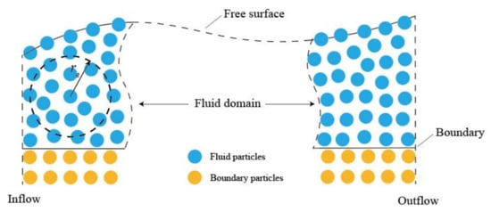
Figure 1.
Boundary conditions in MPS.
3. Improvement
In recent years, increasingly more researchers have proposed new modifications to further improve the accuracy and stability of the MPS method. In this section, the main improvements will be summarized, including operators regarding to interpolation, gradient and Laplacian operators, pressure solving, boundary conditions and regularization of particle distribution.
3.1. Discretization Operators
The interpolation, gradient and Laplacian of the field functions is fundamental and important in any numerical methods, regardless of whether they are meshless or mesh-based. In meshless methods, the kernel function plays an important role in all those discretization operators. For MPS method particularly, instead of using the kernel function as the weight function for particle interactions with it differentiated for gradient and Laplace operators as in the SPH method, the discretization of the gradient model and the Laplace also has kernel function itself involved as in Equations (14)–(16). In the sections below, we summarize the new developments for these discretization operators.
3.1.1. Different Kernel Functions
At present, the most widely used kernel function is still the original one proposed by Koshizuka [1], as in Equation (7). The main characteristic of this kernel is that when two particles are getting close to each other, the value of the function will increase to be infinity, so that the repulsive forces between the particles are also of a larger value, which helps avoid local aggregation of particles.
However, in violent flow simulations, the distance between particles can be small, which causes excessive repulsive forces between neighboring particles. This can, therefore, adversely perturb the motion of the fluid particles, which will in turn affects the accuracy and stability of the simulations. To tackle this problem, Zhang et al. [11] introduced a kernel function (Equation (17)) similar to the original one but without singularities, and this new kernel is proved to be effective in avoiding singularity at .
There exist some other forms of kernel functions. Ataie-Ashtiani et al. [29] compared six different kernel functions in terms of the numerical accuracy and stability of the MPS method for simulating the dam-break problem. In his research, the exponential, cubic spline, quartic spline [30], B spline [31] and two kernels used in MPS by Koshizuka et al. [1,28] are examined. The results show that the kernel used by Shao et al. [31] (Equation (18)) is more accurate and stable in the simulation of dam-break:
3.1.2. Gradient Model
The non-conservation of momentum and spurious pressure fluctuations have been reported to be two major drawbacks of particle methods [32]. Although the use of minimum pressure in Equation (14) is essential to avoid the so-called tensile instability issue, it violates the momentum conservation law. Various pressure gradient operators have been developed to enhance the momentum conservation and stability.
- Linear momentum conservation
In the original MPS, the pressure gradient forces between a pair of particles do not satisfy the Newton’s third law (i.e., the action must be equal to the reaction), which means the momentum will not be exactly conserved during the simulation. Thus, there are some modifications for the gradient operator to enforce the linear momentum conservation. The representative work is the one proposed by Khayyer et al. [32,33] as follows:
where
Since the original MPS method assumed that the variation of pressure between particle and neighboring particle is linear in the short distance, Equation (19) corrects the pressure gradient term by replacing in Equation (14) with and replacing with , to form an antisymmetric equation. This equation results in complete conservation for linear momentum and almost exact conservation for angular momentum. The method will be referred to as corrected MPS (CMPS).
Although conservations of linear and angular momentum are almost satisfied, Mondragon argued in [34] that this gradient operator and its corresponding pressure gradient force vector term may lead to an overestimation of interparticle pressure, which introduces unphysical fluid motion and perturbations. Moreover, the instability problem arising from the difference of the particle number densities between the fluid and the wall particles is not considered. The following modification was, therefore, made:
The above equation tackles these issues by adding the interaction term between the pressure minimum of particle and the pressure minimum of particle to the pressure gradient force term. This expression is able to generate a stable pressure gradient force for the non-uniformly distributed particles. The contribution of the average density is also added to the pressure gradient force vector term to correctly model the fluid–wall interface. It not only satisfies the conservation of momentum between particles, but also has sufficient stability.
- Pressure gradient accounting for stabilization
In the original and many modified versions of MPS, the stress instability still remains a problem. It can be classified into tensile instability, which occurs when the interparticle attractive force increases, and compressive instability, which occurs when the repulsive force decreases as the particles get closer [35].
To accurately approximate the pressure gradient and minimize the numerical perturbations in particles’ motions, Khayyer and Gotoh [35] proposed a pressure gradient corrective matrix by considering the Taylor series expansion of pressure between particle and particle . The corrected gradient model yields:
where the corrective matrix in 2D is as follows:
and
Although the above equation does not exactly satisfy the momentum conservation, the numerical errors might be less than those arising from other approximation of pressure gradient, especially where negative pressures present. However, the stability of Equation (21) is generally not guaranteed, as pointed out by Gotoh and Khayyer [20]. Thus, Duan et al. [36] introduced particle stabilizing term (PST) into Equation (21) to overcome the instability problem. The improved pressure gradient model using PST is:
where ξ is a coefficient to adjust the PST strength dynamically:
Since Equation (24) allows dynamic adjustment of the pressure gradient, the stability could be maintained without the need to set negative pressure as zero [36].
Tsuruta et al. [37] proposed a dynamically stabilized (DS) gradient operator comprising the original Taylor-series consistent gradient model and a meticulously adequate stabilizing force. It can be rewritten as:
where is the stabilizing force for the target particle from neighboring particle . The above equation can accurately provide sufficient interparticle repulsive forces to maintain a simulation stable based on the particle distribution.
For the solution of particle pressure gradient on free surface, another approach that can be taken is with virtual particles while adopting the same formula as the conventional gradient. When the virtual particle pressure is zero, the following formula (Equation (27)) can be obtained [38]:
From Equations (19)–(27), it could be regarded as a type of particle redistribution with the purpose to maintain a more regular particle distribution, which is essential to the interpolation accuracy [36,37].
In the computational gradient model, under some circumstances, the distance between particles may be zero, which leads to the failure of the computational result. To avoid the problem due to the presence of zero directional distance, a new pressure gradient calculation method [39] is given. It introduced a new directional weight function based on the radial distance, which is the one-dimensional directional distance. By introducing the new directional weight function (Equation (28)), the denominator of the gradient becomes a function of the radial distance instead of the directional distance . Therefore, the problem caused by the presence of zero in the denominator is prevented.
Equation (28) contains a new variable named ‘‘directional particle number density’’, which is shown in Equation (29). It should be noted that the newly introduced directional particle number density is not related to the physical density.
The above method provides a modified pressure gradient equation only for the problem where the particle directional distance is zero. In more recently developed MPS methods, particle collision models are also used to table similar issues.
Liu et al. [40] introduced dummy particles to stabilize the renormalized Laplacian model on free surface and to enforce the free-surface condition (Equation (30)). The applicability of the pressure gradient model (proposed by Khayyer and Gotoh [35]) is expanded by the Taylor series expansion.
It should be noted that the new gradient model with a dummy particle is only used for pressure gradient calculation and momentum is not exactly conserved.
In addition, the least squares moving particle semi-implicit (LSMPS) method is an arbitrary high-order meshfree Lagrangian approach proposed by Tamai and Koshizuka [41]. Since LSMPS can achieve high-order accuracy for arbitrary particle distribution, it is effective to apply it for gaining a more accurate pressure gradient and it will be discussed later in Section 3.1.4.
3.1.3. Laplacian Model
The original MPS method applies a simplified Laplacian operator based on the concept of diffusion. To stabilize the pressure calculation in the MPS method, applying a more accurate Laplacian model for solving the PPE is one of the challenges.
- Taking divergence of the SPH-type gradient operator
Khayyer et al. [42] pointed out that the Laplacian model can be defined as the divergence of the gradient, which is mathematically consistent. The gradient at a target particle can be expressed in the form of the SPH method [43]. By considering the original kernel (Equation (8)), the high-order Laplacian (HL) in 2D can be obtained as follows:
When Equation (31) replaced the standard Laplacian model for solving PPE, it showed enhanced performance in high strain problems and violent free surface flow simulations.
Khayyer et al. [44] extended the abovementioned 2D Laplacian model to 3D.
However, the incompleteness or inconsistency of the SPH gradient model becomes a source of problem in the HL scheme, which results in inaccuracies especially around the boundaries. Therefore, Ikari et al. [45] derived a correct higher-order Laplace model (CHL) by correcting the gradient based on the Talyor-series expansion. The corrective matrix is firstly applied for gradient of the target particle (Equation (33)) and the CHL scheme is then obtained by taking the divergence of the corrected gradient (Equation (34)):
where
and detailed derivation can be found in Refs. [42,44,45].
- Taking divergence of the MPS-type gradient operator
Ref. [46] assessed the accuracy of the original MPS and proposed a series of modified Laplacian models. Although in most cases, the original Laplacian model performs well, inaccuracies may rise where the diffusion effect dominates. For example, the original Laplacian model may lead to an overestimation of heat conduction when applied to the energy equation. Therefore, Zhang et al. [47] proposed a Laplacian model suitable for heat conduction by solving the divergence of gradient as shown in Equation (36). It enables the Poisson equation to be solved without the parameter , which could cause numerical difficulties.
Likewise, with the idea of solving the divergence of gradient, Xu and Jin [48,49] introduced an improved Laplacian model (ILM) to enhance the performance in the MPS as follows:
where
One can see the detailed derivation in [49]. The Laplacian model of ILM (Equation (37)) has shown better performance in the diffusion problems and Couette flows.
- Other Laplacian operators.
The Moving Least Square method is also applicable for the Laplacian operator. As Ng, K C et al. [46] pointed out that the Least Square approach needs five and nine elements in the base function for 2D and 3D cases, respectively. In Equation (39), fewer elements in the base function are used (three and six for 2D and 3D cases, respectively), which reduces the required number of neighbor particles:
Duan et al. [50] introduced a new Laplacian model by applying a corrected matrix to remove the errors associated with first-order partial derivatives. The corrective matrix in Khayyer and Gotoh [35] can help compute first-order derivatives accurately, but it cannot be directly used in the Laplacian model. Considering the first-derivative errors tend to be dominant compared to the second-derivative ones, a consistent corrective matrix with gradient/divergence models is applied to remove the dominant errors. Therefore, the new Laplacian model can be obtained as:
which enhances the computational accuracy without increasing the cost much.
The zero-density-variation condition and the velocity-divergence-free condition at each full time-step are applied. Hu et al. [51] and Xu et al. [52] introduced new Laplacian operators by discretizing the second-order derivative (Laplacian) directly as follows:
where .
3.1.4. Discretization by Taylor Series Expansion and Least Square Approximation Scheme
In the traditional particle methods, such as SPH and MPS, the function approximation method is a weighted average approach using a predefined kernel function, as well as the approximation of different operators. Accuracy is not satisfactory when the particle distribution is irregular. In addition, local particle-based interpolations by incomplete/inconsistent differential operator models could result in unphysical pressure oscillations [53,54]. Therefore, some researchers have proposed other function approximation schemes that use the weight function, which is essentially similar to the kernel function.
Koh et al. [55] used a new method called the consistent particle method (CPM), where the approximation of derivatives (Laplacian in particular) is obtained by using Taylor series expansion of a differentiable function at a reference particle and solving local matrix equations (Equation (42)) for every particle:
where , ( = 1, 2,…, N), , , , , ,, N is the total number of particles within the support domain of the particle , and is the weight function used in the least square solution to account for the influence of the distance.
Based on the above approach, the pressure Poisson equation and pressure gradient can be obtained by solving Equation (42), which satisfy the incompressibility of the fluid and enable stable calculation. Hence, this method is vital to moving boundaries simulations. The consistency of the algorithm gives good approximation even for irregularly distributed particles.
To improve the simulation accuracy, the discretization of different operators (velocity divergence term, velocity Laplace term and pressure gradient term) must be completed by a particle smoothing program. Hwang et al. [56] developed a novel moving particle method with embedded pressure mesh (MPPM) to provide an accurate and efficient pressure difference equation to achieve a uniform and sufficiently dense particle distribution. In this method, pressure is considered as a field variable rather than a material one moving with fluid flow, which can be approximated with a simple central difference scheme. Therefore, PPE can be written in differential form (i.e., pressure difference equation), which can be solved on grid mesh. Compared with the original particle smoothing method, the results show that the original particle smoothing procedure will yield inconsistent expressions for differential operators, but still predict quite reasonable results in incompressible flow problems, and this smoothed difference format can provide an exact solution that is as precise as the high-resolution finite volume method.
Tamai’s work could be seen as an extension and generalization of Koh’s work [55]. The principle of this so-called least squares moving particle semi-implicit (LSMPS) method is generally described as follows:
- According to Stone–Weierstrass theorem of locally compact version, the approximation of the target function can be gained by a polynomial series locally.
- Utilizing the Taylor expansion of a target point with a nearby point, the approximated polynomial function and the residual of local polynomial approximation can be obtained.
- The weighted least squares procedures are used for new spatial discretization where non-singular weight functions are highly recommended.
- The normal equations equivalent to the existing spatial discretization formulae are derived based on the weighted least squares procedure and with variable transformation according to the abovementioned Talyor series expansion with the residual considered.
- If the residual is expressed by a defined function, after minimizing functional, the normal LSMPS scheme is eventually derived.
When the improved method is applied to benchmark problems, it demonstrates a significant enhancement of stability and accuracy. Tamai et al. [57] focused on the consistency of the second-order derivative approximations for the strong-form particle methods including the LSMPS method, and the convergence of some meshless particle discretization schemes for the Laplace operator. Experiments show that utilizing the new scheme results in more accurate numerical solutions.
3.2. Pressure Solving
The fluid pressure in the MPS method is mainly obtained by solving the pressure Poisson equation, which enforces the incompressibility of the fluid. However, the weakly compressible concept is also adopted in a number of MPS developments. Since the pressure field accuracy has a large impact on the following fluid velocity and particle location update calculations, various developments have been proposed for both weakly compressible and incompressible approaches.
3.2.1. Weakly Compressible Approach
Different from solving pressure implicitly via the pressure Poisson equation in the MPS method, the pressure in the SPH method is solved explicitly by using the equation of state (EOS), which avoids dealing with large matrix when implicitly solving a set of equations for all the particles. Equation (43) is as widely used as the EoS in the SPH method [58]:
where the value of is usually taken as 7 and 1.4 for water and air, is reference density, is pressure, and is the sound speed at reference density.
As the EoS provides a direct relationship between density and pressure, pressure can be solved faster than solving Poisson’s equation at each time step. Consequently, the computational time per time step is greatly reduced by ensuring a certain accuracy of the results.
The incompressibility model in the original MPS is replaced with a weakly incompressible model in Shakibaeinia et al. [59], which uses an MPS original spatial discretization (particle interaction) formula. Therefore, the EoS is applied to solve pressure at each time step instead of the Poisson equation, which is written as:
A new Moving Particle Explicit (MPE) method [39] has been developed by combining the weakly compressible SPH (WCSPH) [58,60] and the original MPS. Similar to the MPS method, the concept is based on a weighted averaging scheme, where a directional particle number density is introduced and the spatial discretization is derived without imposing any simplifications. The procedure is similar to the WCSPH method. Considering the slight compressibility, the continuity equation and the equation of state (Equation (43)) are used to solve velocity and pressure, which makes the method fully explicit.
3.2.2. Incompressible Approach by Solving PPE
- High-order scheme in the time domain
In the work of Hu et al. [51] and Xu et al. [52], PPE with different source terms under both the zero-density-variation condition and the velocity-divergence-free condition at each full time-step are given. In the framework of fractional time-step approach, which is based on the projection algorithm, different forms of PPE are obtained. Under the condition of zero-density-variation, the PPE are given as:
where is the inverse of the particle volume. With Equation (41), the following equation is obtained:
Similarly, under the velocity-divergence-free condition, the PPE can be discretized as:
where is the normalized vector pointing from particle to and is the viscosity for the particle.
In the work of Hu et al. [51], the first prediction step is to calculate the intermediate particle velocity at the half-time step and also the full-time step, from which the intermediate particle location at full time step is obtained. Afterwards, in the second correction step, the particle location is modified to satisfy the zero-density-variation condition and particle velocity at the full time step is modified by enforcing the velocity-divergence-free condition. However, this scheme has to solve the pressure Poisson equation twice, which is more time consuming.
- New types of PPE source terms
The source term of PPE is an important factor that may lead to pressure oscillations and corresponding error accumulation. Based on the divergence of the intermediate velocity and the variation of particle number density, there are two forms of source terms in the PPE, namely the DI type and DF type. To improve the stability, some researchers applied different mixed source terms which combine DI and DF types. These new types of PPE source terms both consist of a main part and error compensation terms. Typical expression are as follows:
where , , and are the coefficient and have different values and expressions in various studies.
In summary, the first term of the right-hand side of the above equation is the expression of original PPE (i.e., DF type), the second term is the error compensation of particle number density (i.e., DI type), and the third term is the artificial compressible compensation. These types of source terms ensure smooth pressure distribution in both space and time with the fluid incompressibility maintained.
ISPH (Incompressible Smoothed Particle Hydrodynamics) applies the divergence on both sides in the correction step, and then obtains the original PPE based on the zero fluid velocity divergence for incompressible fluids. By combining the advantages of the PPE of MPS and ISPH, Tanaka et al. [61] proposed a mixed source term method, which was further improved by Lee et al. [62], where , , . Sun et al. [63] proposed a criterion for determining coefficient for the Poisson equation with mixed DI and DF source terms as follows:
Then, Tanaka et al. [61] proposed a quasi-incompressible term in Poisson’s equation to improve the stability of numerical simulation, which adds an artificial compressible compensation to the right-hand term of the PPE. In this method, the coefficients are selected as , , .
In [64], the pressure field is solved from an improved PPE. The divergence of is discretized by the high-order source (HS) formulation [42]. The mixed source term consists of both the divergence-free and constant-PND (particle number density) conditions and the artificially compressible model, which is widely applied in MPS [33,61,64,65]. Therefore, is the relaxation coefficient from 0.01 to 0.05, and is the artificial compressibility coefficient from to .
To improve the accuracy of pressure calculation, Khayyer et al. [33] replaced the source term in the PPE with the temporal varied particle number density involved. Furthermore, a higher-order source term expression (Equation (51)) is obtained by calculating the material derivative of the kernel function. Compared with the traditional source term methods, the high-order source term method can effectively suppress the pressure oscillation, but near the wall boundaries it still has the problem of local pressure oscillation.
Thus, an improved source term expression is proposed considering error compensation of the source term, as shown in Equation (52). In this formula, two error mitigation terms are added on the basis of the high-order source term, one of which represents the instantaneous change of particle number density, and the other represents the deviation of particle number density from the initial value:
where and
Though more accurate and stable pressure calculation is achieved by Equation (51), there still exist unphysical pressure oscillations in simulations of sloshing flows. Kondo et al. [66] discretized the density term in the mixed source term into a main part and two error compensation parts and smooth pressure distribution is obtained by adjusting the two compensation coefficients.
To maintain the momentum conservation for interparticle collisions, Cheng et al. [67] proposed the time-scale correction of particle-level impulses (TCPI) as a new source term for the PPE. With this approach, the non-physical pressure oscillations dramatically reduced.
where is a relaxation coefficient and the superscript is for variables after the correction for the intermediate physical quantities.
Non-physical pressure oscillations usually arise due to temporal inconsistencies in the source terms of the PPE, as well as the overestimated magnitudes of the pressure gradient force vector terms. The parameter in the Laplacian operator is mathematically to reduce the error caused by replacing the infinite Gaussian function with the truncated kernel function. When virtual particles [34] are introduced in MPS method, the parameter needs to be redefined to account for the virtual particle number density difference of the PPE. Equation (57) gives the new definition of virtual parameter , where the first term is the integrated value of the spatial variance distribution of the equation, and the second term is the proposed modification of the variance that depends on the velocity. The source term of the PPE is now modified as Equation (56):
By adding virtual particles beyond the free surface, Ref. [38] modified the PPE and the pressure gradient term. The left-hand side is divided into two terms for the actual particles and virtual particles in Equation (58), where is a scalar parameter for stabilizing the simulation and is the initial fluid density.
In order to improve the numerical stability and suppress the numerical diffusion in long-term computations, Xu and Lin [68] proposed a new two-step projection method (NTSPM), as expressed in Equation (59). is a weighting factor that vary from 0 to 1. If = 1, it maintains the same as traditional two-step projection method with the pressure at the next time step solved according to intermediate velocity only. = 0.5 is used to equally account for the pressure contribution at time steps and , which is similar to the second-order central time difference scheme for pressure. By comparing with traditional methods, the main difference is the use of in calculating the intermediate velocity, and another difference is that the solution of velocity and pressure at state F is changed from the assignment to interpolation [47,69,70,71]. Here, the state F is when the particle position is updated and , , and at time () are obtained by calculating the interpolation from , , and , respectively. In state F, the particle is only assigned to a new position, and the velocity is not updated, so the divergence of the velocity is not zero.
3.3. Boundary Conditions
The boundary conditions need to be considered to ensure the closure of the Navier–Stokes equation. Several important developments have been made with respect to free surfaces, solid boundaries and import and export boundaries. These models have been demonstrated to be effective and practical for complex geometries, which help reduce computational costs and increase stability.
3.3.1. Free Surface Identification and Conditions
In the original MPS method, the pressure of the free surface particles is assigned a value of zero. As a result, there is no repulsive force between the free surface particles, which can lead to aggregation and overlap of free surface particles, reducing the accuracy of the free surface calculation. In addition, internal particles may also be misidentified as surface particles, resulting in pressure oscillations and even failure in severe cases. There have been more advances in the accuracy of free surface detection and pressure implementation.
- Surface particle identification
- (a)
- Using the number of neighboring particles
In the original MPS method, there are many falsely identified particles inside the main fluid body when particles are not evenly distributed due to sensitive particle number density. One modification [61,62] is to use the number of neighboring particles within its support domain instead of particle number density (). In this method, the criteria for the number of neighbor particles is set as:
where is the initial number of neighbor particles. The number of neighbor particles is defined as:
where is a weight function for surface detection and is formulated as:
- (b)
- “ARC” type
Another approach is proposed by checking whether the “arc” of the particle is fully surrounded by its neighbor particles [55]. If the arc with radius is completely covered by the arcs of its adjacent particles, it will be identified as an internal particle. On the contrary, if there is a gap on the arc, it is identified a free surface particle. Compared with the particle number density method, this method can largely avoid misidentification caused by slight clustering and can judge the free surface more accurately. However, this method needs to verify the arc of each fluid particle, and the calculation is more complex. Sun et al. [8] simplified this checking progress by splitting the circle into 360 segments evenly distributed along the circle. If all these points are covered by the circles of its neighbor particles, the center particle is then regarded as an inner particle. As shown in Figure 2, particle A is a free surface particle and particle B is an inner particle.
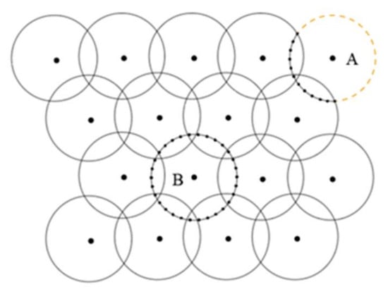
Figure 2.
“Arc” type for 2D case in Refs. [8,55].
- (c)
- Relative position vector
There are also works employ a detection method [72] based on the asymmetry distribution of neighboring particles, expressed as follows:
If the absolute value of the function at particle is greater than a threshold as , then particle is considered as a free surface particle. The method is based on the ground that the equation is equivalent to the mass gradient when multiplied by the mass of the particles which should be close to zero. In addition, this method allows a more accurate description of the particle asymmetry, which omits the calculation of the number density of intermediate particles on the free surface and speeds up the calculation.
- (d)
- Check distribution of neighboring particles
Under the original free surface identification conditions, particles inside the fluid may be identified as free surface particles. In [34], firstly, a group of possible free surface particles are identified according to Equation (64), then the internal particles are ruled out by if all neighbor particle within the support domain of particle satisfies Equation (65):
This method combines particle number density condition and effectively reduce the phenomenon of false judgment. However, the calculation process is more cumbersome and reduces the calculation efficiency.
- Free surface conditions implementation
In the original MPS method, zero pressure is applied on the identified free surface particles. However, there are also papers that solve the surface pressure based on the PPE with virtual particles added beyond the surface whose pressures are assigned as zero. In these works, the virtual (or conceptual) particles only change the particle number density of free surface particles without their positions used in the modified PPE as shown in Equation (66) [36,73]. Virtual particles also contribute to complete the support domain for surface particles when pressure gradient is calculated which significantly increase the accuracy of velocity and position update. The modified PPE is in the following the form:
The position of the virtual particle is determined based on the distribution of the surrounding particles of those density is lower than n0. The virtual particle will only participate in the Laplacian discretization of targeted particle, but not change the source term nor affect other particles. The zero pressure is imposed on virtual particle rather than targeted free surface particles [73,74,75].
3.3.2. Solid Boundary Conditions
Despite the widespread applications of the MPS method, it remains a challenge to accurately model boundaries (fixed or moving) and fluid–boundary interactions.
The methods treating solid boundaries in particle methods can mainly be divided into three categories. The most widely used approach is the ghost particles (or dummy particles) which are originally introduced by Koshizuka and Oka [76]. This treatment can effectively avoid particle penetration, but it increases computational cost and is difficult to apply for complex shaped boundaries. In this method, the solid boundary consists of one layer of wall particles and two layers of ghost (dummy) particles beyond the wall. The wall particles are positioned along the solid boundary, and the dummy particles are placed just outside of the wall particles to compensate for the deficiency in particle number density. Shakibaeinia and Jin [59] employed the ghost particles method by imposing a tangential velocity component on the fixed ghost particles while the normal velocity component is maintained zero, which makes it capable for the free-slip condition (Figure 3).
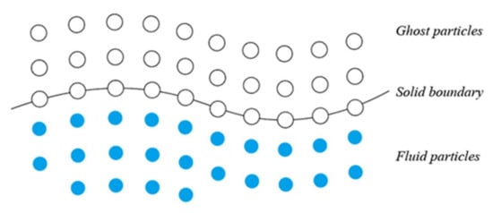
Figure 3.
Solid boundary with ghost particles in Ref. [59].
Xie et al. [77] implemented the no-slip condition by the linear interpolation of the velocity of the nearest liquid particle and solid particle so that the velocity at the mid-point between these two particles (where the solid surface is) is zero. Thus, the solid boundary is represented at the center between the solid particles and the first layer of fluid particles. Therefore, the velocity of a solid particle is modified by a fluid particle velocity as:
where is the distance between the solid particle and the solid surface and is the distance between the solid particle and fluid particle.
Later, Lee et al. [62,78] imposed moving mirror particles positioned normal to the wall boundaries instead of being fixed. Moreover, the mirror particles are updated every time step according to the fluid particles, so that the Neumann boundary condition can be strictly satisfied. To further reduce the computational effort, Park and Jeun [79] developed the temporary mirror particles, which use mirrored fluid particles to replace the initially placed mirror particles.
The boundary force approach proposed by Monaghan [58] models the fluid–wall interaction in a way similar to that of the Lennard–Jones model, which generates a force in the direction of the centerline of the two particles when a fluid boundary particle becomes a neighbor particle to inside fluid particles. However, due to the boundary force, fluid particles may experience a non-uniform normal force and a non-zero tangential force along a solid boundary. To tackle this problem, a tangential factor was used to correct the interaction force, enforcing it as normal to the boundary by involving the perpendicular distance from the boundary only [80,81]. In addition, some other methods have been introduced such as a refined radial force model [82] and the normalizing function [83,84], which imposes correction when particles go beyond the boundaries.
Although there are successes of handling solid boundaries, they increase the complexity of modeling and compromise computational accuracy. Kulasegaram [83] and Ferrand et al. [85] proposed a unified semi-analytical wall boundary condition, which depends on the local shape of a wall. Leroy et al. [86] developed the ISPH by using the unified semi-analytic boundary model under the consideration of a non-homogeneous Neumann wall boundary condition [87] for the viscous term. Manenti et al. [88] introduced a semi-analytic approach for modeling solid boundaries in SPH by considering them as continuum material with a proper distribution of velocity and pressure, which was successfully applied to sediment flow.
Fadafan and Kermani [89] proposed a simple form for curved wall boundaries using a single parameter () together with an auxiliary function. If the number of fluid particle in the vicinity of particle is more than or equal to 1, the value of criterion parameter for the wall is half the value of fluid; otherwise, it is equal to the value of fluid. This simple method reduces particle numbers and saves CPU time.
Complex wall geometries are hard to be represented in most MPS applications. Zhang et al. [90] used the triangle meshes to represent the complex wall geometries and the wall boundary conditions on the triangle mesh are implemented by the polygon wall boundary conditions (PW). In this method, the pressure at the wall boundary (Equation (68)) is derived from the Neumann boundary condition and a first-order gradient model is applied, which help improve the accuracy and stability. The result shows this method is capable of maintaining numerical stability for complex geometries.
where is the module of the distance vector from a fluid particle to the balance position and the distance from this position to the boundary is a constant value, is the module of the distance vector from particle to the solid boundary, is the wall contribution of fluid particle to the particle number density, and is the minimum pressure within support domain of particle .
Based on the least square MPS (LSMPS) scheme, Matsunaga et al. [91] proposed a new approach to easily handle no-slip and free-slip wall boundary conditions where wall geometries are represented by line segments in 2D and polygons in 3D. The wall boundary conditions are inserted into the differential operators for fluid particles near the wall. Therefore, the Neumann boundary conditions can be fully satisfied:
where and is a unit normal vector to the wall and the moving velocity of the wall.
In the study of Matsunaga et al. [92], a novel wall boundary treatment adopting analytical volume integration is presented. Without any boundary particles, the advantage of this method is that it does not require high calculation cost nor compromise accuracy. However, the applicability of the present method is limited to 2D problems.
3.3.3. Import and Export Boundary Conditions
In the numerical simulation of practical engineering problems, the boundary conditions of the inlet and outlet are ones of the most common boundary types.
A commonly used technique for the import and export boundary is to divide the import region, the flow region, and the export region in the flow field. In the import region, the velocity of the particles is set based on the import boundary conditions, and the pressure is set based on the pressure interpolation of the neighbor particles in the flow region. After the particles enter the flow region from the inlet region, the particles are driven by the interparticle interaction forces calculated from the flow field. As the particles usually move from the import to the export, new particles need to be added to the import region depending on the number of particles leave. It is relatively easier to implement the export boundary condition as it is not necessary to add new particles during the flow [93].
Although the inlet and outlet boundary treatment techniques above are simple and easy to implement, it is difficult to ensure the conservation of mass in the flow field due to the variation of the number of particles entering and leaving the flow field and may cause significant oscillations in the pressure field.
Shakibaeinia and Jin [59] introduced a particle recycling strategy for inflow and outflow boundaries by an extra type of particle called storage particles, which carry no physical values, such as position, velocity, or pressure. When particles enter the simulation domain, they are fluid particles with physical properties added depending on inflow boundary condition by Equation (71). When particles leave the simulation domain, they are changed to storage particles, and all the physical properties of particles are removed.
where is average particle distance and is velocity component in y-direction.
Hosseini and Feng [87] proposed a pressure modification algorithm by replicating the first line of fluid particles three times upstream at the entry. For those entry layers, the Neumann condition is implemented. When a particle moves out of the entry layer, it becomes an inner fluid particle. Similarly, the last layer of fluid particles is replicated and placed downstream of the exit (i.e., the exit layer) with the Dirichlet condition is satisfied.
Leroy et al. [94] imposed an open boundary condition based on the unified semi-analytical boundary conditions. Equation (72) allows particles to enter the domain through a boundary with prescribed velocity (i.e., inlet boundary), and to leave the domain through a boundary with prescribed pressure (i.e., outlet boundary):
where , , and are the velocity, temperature, and a unit normal vector, respectively, and the superscripts denote the value of a field at an open boundary with prescribed velocity/pressure.
Shibata et al. [95] developed a transparent boundary condition consisting of two columns of square cells for simulating water waves, as shown in Figure 4. The outer cell column named “A-type” is for the inflow, where particles are generated, and the inner cell column named “B-type” helps determine the position of the particles generated in the A-type cells. A new particle will be generated in A-type cell when it is vacant, but if the center position of the A-type cell is over the approximated wave surface, the particle will be placed at a distance from the neighboring particles located in the next B-type cell.
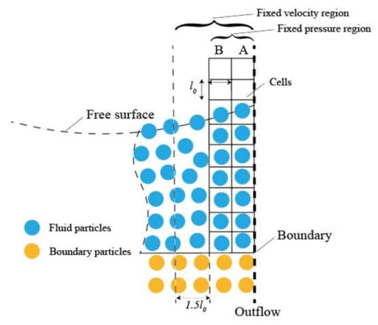
Figure 4.
The transparent boundary in Ref. [95].
By using boundary particles and modifying their physical values, Hu et al. [96] proposed three kinds of inlet/outlet boundary conditions: a pressure specified inlet/outlet condition, a velocity profile specified inlet/outlet condition, and a fully developed flow outlet condition. Compared with the finite volume method, this approach exhibits accuracy and numerical stability.
3.4. Regularization of Particle Distribution
The motion of particles may lead to non-uniform particle distributions, which consequently causes spatial discontinuities when discretizing the PPE and corresponding inaccuracies in the pressure calculation. Therefore, it is necessary to use particle regularization technique to improve the particle distribution and mitigate non-physical pressure oscillations.
3.4.1. Particle Shifting Scheme
In Lagrangian particle methods, particles moving along the streamlines may lead to particle clustering or scattering even when the Lagrangian-form N–S equations are solved accurately. Therefore, the redistribution of particles is necessary to maintain stability.
Particle shifting proposed by Xu et al. [52] shifts particle positions in the ISPH method. In this method, the expression for position shift is based on the particle convection distance and the particle size, as shown by Equation (73). Moreover, physical quantities need to be interpolated at the new position by the Taylor series according to Equation (74), where is a constant, set as 0.01–0.1, is the shifting magnitude, and is the shifting vector:
Lind et al. [97] generalized the particle shifting approach of Xu et al. [52] and imposed a shifting algorithm based on Fick’s law of diffusion as shown in Equation (75), where the concentration is expressed by the sum of the kernel function:
Apart from shifting the particle positions, the artificial pressure-like function in Monaghan [98] is applied in the calculation of the concentration gradient. Additionally, suggestions are given on choosing an appropriate diffusion coefficient.
As mentioned above in Equation (26), Tsuruta et al. [37] introduced a dynamic force in the particle motion. This dynamic force can avoid particle aggregation. Despite the overall distribution being improved, there exists a drawback that the force component between different particles can affect each other and cause a not fully uniform distribution.
Particle dispersion may occur where there is insufficient particle number density, especially around free surface. In order to reproduce the physical motions of free surface particles, Tsuruta et al. [74] defined the space potential particles (SPP) to fill the void between surface particles, as shown in Figure 5. Its location is calculated by Equation (76), where is the relative coordinate vector of the centroid of neighboring particles to particle and is the kernel function in the MPS (Equation (7)). A more realistic physical field, where repulsion and tension are balanced, is gained by applying this scheme into pressure Poisson equation and pressure gradient.

Figure 5.
The space potential particles in Ref. [74].
In Hu et al. [99], two particle redistribution models are developed. The first one is called the “spring model”, which moves particles to some place near the position obtained by Lagrangian convection. The second one is called the “static model”, which can simply move particles back to the original position and fix them.
PST (particle stabilizing term) and PS (particle shifting) are similar in terms of modifying particle distribution through modifying different fields with PST adjusting the velocity field whereas PS adjusting the position field. Another difference between the two approaches is the criteria to determine whether the adjust to take place. For PST, it relies on a local pressure difference . However, it is possible that the particle distribution is seriously distorted but remains small, for which PST fails to be triggered and it causes instability. Considering the similarity between PST and PS, Duan et al. [50] introduced the following PS for MPS:
3.4.2. Background Pressure Mesh
Some researchers also suggest that the performance of particle method can be greatly improved by combining the use of background mesh, where pressure is calculated and the particles are advanced in Lagrangian frame as the original particle method [25,100]. Hwang et al. [100] proposed a moving particle method with embedded pressure mesh (MPPM) to help obtain an accurate pressure field. Using the finite-volume method, the continuity equation can be discretized on this regularly distributed and fixed mesh. Then, considering the momentum interpolation for the collocated grid and the concept for the ALE grid, the velocities in the continuity equation can be further approximated with a simple center-difference operator. Finally, substituting these velocities into the continuity equation which is discretized on meshes, the equation for the pressure can be successfully obtained. With the aid of the inserted regular mesh, the pressure can be calculated accurately without particle smoothing procedures for the PPE and operators. After that, the velocity and position information of the particle at the next time step can be calculated by the pressure field.
Ng, K.C., et al. [101] further developed the MPPM method to the Unstructured Moving Particle Pressure Mesh (UMPPM) method, aiming to extend the MPPM solver to handle arbitrarily shaped flow boundaries. In this work, the body-fitted unstructured mesh is selected to replace the Cartesian pressure mesh employed in the original MPPM method. In addition, a consistent Laplacian model, namely the Consistent Particle Method (CPM) is incorporated in the UMPPM for the viscous stress term in an implicit form. The results shows that this new method can address the limitation of the MPPM method in handling arbitrarily shaped flow boundaries effectively.
Liu et al. [102] improved the accuracy of MPPM method and proposed the Mixed Lagrangian-Eulerian (MLE) method. In this method, the momentum equation is discretized on the moving particles, while the continuity equation is on the uniform Cartesian grid points. On the one hand, the Laplacian term on the background mesh can be approximated by using a higher-order scheme, which are then interpolated to the particles. On the other hand, with the pressure and velocity are obtained on the Eulerian mesh, spatial derivative terms such as pressure gradient, the velocity Laplacian and velocity divergence can be calculated. With this MLE method, higher accuracy is attained and convective instability can also be avoided.
Wang and Khayyer et al. [103] proposed a Background Mesh (BM) scheme to provide an accurate, smooth and spatially continuous overall source term for the PPE. With the interpolated velocities at fixed and perfectly regular neighboring nodes, the source terms are firstly calculated at background mesh nodes, which are then interpolated to the nearest neighboring particles. The background mesh is only applied for the PPE source terms to provide spatial continuity, while other terms and equations are solved in the Lagrangian framework. Hence, this scheme keeps the merits of Lagrangian mesh-free methods and allows for more stable and accurate pressure calculations.
3.4.3. Initial Particle Distribution
As the particles are discretized, fluid particles can easily move under pressure gradients, which may, therefore, lead to discontinuous changes in the particle number density distribution, which becomes more pronounced in three-dimensional simulations.
Figure 6a shows the initial particle distribution called simple cubic (SC) arrangement, where all the fluid particles are uniformly arranged. However, the filling rate of this arrangement is relatively low. Natsui et al. [104] introduced the checker-board (CB) arrangement, a uniform particle arrangement with a high filling rate. A similar approach was also attempted in the SPH method.
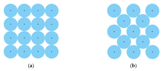
Figure 6.
Variation of particle arrangements in different initial conditions in Ref. [104]: (a) Simple Cubic (SC); (b) Checker Board (CB).
Colagrossi et al. [105] proposed a particle parking algorithm for initial particle distribution. Firstly, the free surface is treated as a solid boundary and the domain boundary is modeled by fixed particles with zero velocity. Then, the density, pressure and volumes are constant for the whole fluid domain so that the continuity equation can be neglected. Therefore, with the initial particle pressure, the hydrostatic pressure, particle position, and other physical quantities can be computed.
3.4.4. Local Particle Refinement
In the MPS method, local particle refinement techniques are mainly categorized into the multiresolution particle technique and overlapping particle technique.
Tanka et al. [106] made the first attempt on multiresolution particle technique based on the MPS method. In this method, particles with different resolutions are applied to particle interaction models and for solving the PPE. Since in the original MPS method, the whole flow field is represented by a single particle resolution, modifications for the particle interaction models for various particle resolutions are needed. Thus, Tanka et al. [106] employed particle diameters to modify the particle action model and to determine the correction factor for the kernel function. Meanwhile, in order to avoid the inaccuracy of particles number density caused by different resolutions particles, velocity divergence is fully contributed to the source term of PPE. By adopting the algorithms of the muti-resolution based on the original MPS method and also the LSMPS method, the method has been tested for a number of benchmarks (channel flows and free surface flows) and demonstrates its robustness in low computational costs.
The overlapping particle technique (OPT), proposed by Shibata et al. [107], can help avoid the direct interaction between particles with different resolutions. Similar to mesh-based methods, the whole computational domain, including the overlap domain, is filled with coarser particles and the local domain, i.e., the overlap domain, is filled with finer particles. Within one time step, firstly the coarser particles are used to solve the flow field. Then, the pressure and velocity will be transferred to the boundary of overlap domain, which will be adopted for solving the refined zone. This is a single way coupling procedure with the flow properties in at low-resolution particles transferred to the boundary of high-resolution particles, while no flow information transferred the other way round.
4. Conclusions
Initially proposed in nuclear engineering, the MPS method has already been successfully applied to many other areas, especially in marine and ocean engineering, including violent flows, wave interactions with fixed/floating and rigid/deformable structures, etc. In terms of fluid –structure interaction problems, the MPS method can accurately capture changes in free surface and deformation of structures. Additionally, it has a unique advantage in handling multiphase flow benefits from its strength in dealing with large deformation boundaries when compared to mesh-based methods.
Despite the ability to naturally track the free surface, some drawbacks exist in the MPS method, such as instability, non-physical pressure oscillation, low accuracy, etc. The MPS method has seen substantial improvements over the last 20 years and significant progress has been made in terms of stability, accuracy, boundary conditions, computational efficiency, etc.
Non-physical pressure oscillation is a common challenge in all particle-based methods, for which scholars have proposed numerous effective improvements and made significant progress for the MPS method. In particular, the gradient model, the Laplace operator, and other discretization operators have effectively improved the pressure oscillation problem of the MPS method.
In terms of implementation of boundary conditions, the MPS method benefits from its inherent advance in tracking free surface and dealing with complex boundary geometries. The improvements have been made to remedy the problems of incomplete support domain at boundaries and to improve the accuracy of surface identification. The inlet and outlet boundaries techniques with particle adding and removing schemes are also developed. All those achievements enable the MPS method to be applied to various flow dynamics and flow structure interactions in ocean engineering.
Preventing particles from aggregation during the simulation also significantly affects the accuracy and stability of the MPS method. Shifting particles when they are getting closer is one of the methods to avoid particle aggregation. Alternatively, it is effective to improve the accuracy of the pressure by using a pressure background grid, which can subsequently improve the accuracy in terms of velocity and particle position updates. Improvements have also been made for initial particle distribution to increase the filling ratio and for local particle refinement to efficiently increase the accuracy where necessary.
In summary, with all those improvements, there still exists potential regarding the accuracy, instability, and computationally expensive properties, especially for 3D simulations, when the MPS method is applied to various engineering problems. Another challenge of the particle method is the simulation of multiphase flows with large density ratios at the phase interface. As described above, various methods exist, but some of them conflict with the mass and momentum conservation, and the numerical format is not consistent across the interface. At the same time, development of turbulence models in the MPS is of significant importance for complex flow simulations, either importing as the existing sub-scale particle scale (SPS) model developed for SPH method [108,109] or proposing new formulations for the MPS method, and the CFD models in the mesh-based method can serve as references to develop robust turbulence models for the particle method.
Author Contributions
Conceptualization, Z.S., L.-Y.D., S.-Y.T., Z.-K.X., K.D. and Y.Z.; investigation, Z.S., L.-Y.D., S.-Y.T. and Z.-K.X.; resources, Z.S.; data curation, L.-Y.D., S.-Y.T. and Z.-K.X.; writing—original draft preparation, Z.S., L.-Y.D., S.-Y.T. and Z.-K.X.; writing—review and editing, K.D. and Y.Z.; supervision, Z.S.; project administration, Z.S.; funding acquisition, Z.S. All authors have read and agreed to the published version of the manuscript.
Funding
This work is supported by the National Key Research and Development Program of China (2021YFC2801701 and 2021YFC2801700), National Natural Science Foundation of China (52171295), Open Project of State Key Laboratory of Deep Sea Mineral Resources Development and Utilization Technology (SH-2020-KF-A01), Young Scholar Supporting Project of Dalian City (Grant No. 2020RQ006), and Fundamental Research Funds for the Central Universities (DUT22LK17, DUT2017TB05), to which the authors are most grateful.
Institutional Review Board Statement
Not applicable.
Informed Consent Statement
Not applicable.
Conflicts of Interest
The authors declare no conflict of interest.
Nomenclature
| a | A gradient vector |
| C | Color function value or a coefficient |
| C | Corrective matrix |
| Cp | Specific heat capacity |
| d | Number of spatial dimensions |
| F | Force |
| g | Gravity |
| G | Gaussian function |
| k | Conductivity |
| l0 | Initial particle distance |
| L | A matrix |
| m | Mass |
| n | Particle number density |
| n | A normalized vector |
| n0 | Standard value of particle number density |
| P | Pressure |
| re | Cutoff radius |
| r | Particle position vector |
| r | Distance |
| t | Time |
| T | Viscous stress tensor |
| u | Horizontal velocity |
| u | Velocity vector |
| ν | Vertical velocity |
| w(x) | Weight function |
| x | Position |
| α | Weighing factor |
| β, γ | Coefficients |
| γ | Surface tension force |
| δ | Dirac function |
| Δ | Increment |
| η | Weight coefficient |
| κ | Curvature |
| λ | Coefficient of Laplacian mode |
| μ | Dynamic viscosity |
| Π | Adjusting parameter |
| ρ | Fluid density |
| σ | Surface tension coefficient |
| ϕ | A scalar quantity |
| φ | A vector |
| Subscripts | |
| G | Gaussian function |
| , | Particle identification number |
| Supscripts | |
| DS | Dynamic stabilization |
| k | Time step number |
| * | Temporal value |
References
- Koshizuka, S.; Oka, Y. Moving-Particle Semi-Implicit Method for Fragmentation of Incompressible Fluid. Nucl. Sci. Eng. 1996, 123, 421–434. [Google Scholar] [CrossRef]
- Li, G.; Gao, J.; Wen, P.; Zhao, Q.; Wang, J.; Yan, J.; Yamaji, A. A review on MPS method developments and applications in nuclear engineering. Comput. Methods Appl. Mech. Eng. 2020, 367, 113166. [Google Scholar] [CrossRef]
- Luo, M.; Khayyer, A.; Lin, P. Particle methods in ocean and coastal engineering. Appl. Ocean Res. 2021, 114, 102734. [Google Scholar] [CrossRef]
- Hwang, S.-C.; Khayyer, A.; Gotoh, H.; Park, J.-C. Development of a fully Lagrangian MPS-based coupled method for simulation of fluid–structure interaction problems. J. Fluids Struct. 2014, 50, 497–511. [Google Scholar] [CrossRef]
- Sun, Z.; Djidjeli, K.; Xing, J. The weak coupling between MPS and BEM for wave structure interaction simulation. Eng. Anal. Bound. Elem. 2017, 82, 111–118. [Google Scholar] [CrossRef] [Green Version]
- Khayyer, A.; Tsuruta, N.; Shimizu, Y.; Gotoh, H. Multi-resolution MPS for incompressible fluid-elastic structure interactions in ocean engineering. Appl. Ocean Res. 2019, 82, 397–414. [Google Scholar] [CrossRef]
- Zhang, G.; Chen, X.; Wan, D. MPS-FEM Coupled Method for Study of Wave-Structure Interaction. J. Mar. Sci. Appl. 2019, 18, 387–399. [Google Scholar] [CrossRef] [Green Version]
- Sun, Z.; Djidjeli, K.; Xing, J.T.; Cheng, F. Coupled MPS-modal superposition method for 2D nonlinear fluid-structure in-teraction problems with free surface. J. Fluids Struct. 2016, 61, 295–323. [Google Scholar] [CrossRef] [Green Version]
- Zhang, G.; Hu, T.; Sun, Z.; Wang, S.; Shi, S.; Zhang, Z. A delta SPH-SPIM coupled method for fluid-structure interaction problems. J. Fluids Struct. 2021, 101, 103210. [Google Scholar] [CrossRef]
- Tsukamoto, M.M.; Cheng, L.-Y.; Nishimoto, K. Analytical and numerical study of the effects of an elastically-linked body on sloshing. Comput. Fluids 2011, 49, 1–21. [Google Scholar] [CrossRef]
- Zhang, Y.-X.; Wan, D.-C.; Hino, T. Comparative study of MPS method and level-set method for sloshing flows. J. Hydrodyn. 2014, 26, 577–585. [Google Scholar] [CrossRef]
- Kim, K.S.; Kim, M.H.; Park, J.-C. Development of Moving Particle Simulation Method for Multiliquid-Layer Sloshing. Math. Probl. Eng. 2014, 2014, 350165. [Google Scholar] [CrossRef] [Green Version]
- Hwang, S.-C.; Park, J.-C.; Gotoh, H.; Khayyer, A.; Kang, K.-J. Numerical simulations of sloshing flows with elastic baffles by using a particle-based fluid–structure interaction analysis method. Ocean Eng. 2016, 118, 227–241. [Google Scholar] [CrossRef]
- Zhang, Y.; Wan, D. MPS-FEM coupled method for sloshing flows in an elastic tank. Ocean Eng. 2018, 152, 416–427. [Google Scholar] [CrossRef]
- Khayyer, A.; Gotoh, H. A Multiphase Compressible–Incompressible Particle Method for Water Slamming. Int. J. Offshore Polar Eng. 2016, 26, 20–25. [Google Scholar] [CrossRef] [Green Version]
- Chaudhry, A.Z.; Shi, Y.; Pan, G. Recent developments on the water entry impact of wedges and projectiles. Ships Offshore Struct. 2022, 17, 695–714. [Google Scholar] [CrossRef]
- Sun, Z.; Jiang, Y.-C.; Zhang, G.-Y.; Zong, Z.; Xing, J.T.; Djidjeli, K. Slamming load on trimaran cross section with rigid and flexible arches. Mar. Struct. 2019, 66, 227–241. [Google Scholar] [CrossRef]
- Sun, Z.; Liu, G.-J.; Zou, L.; Zheng, H.; Djidjeli, K. Investigation of Non-Linear Ship Hydroelasticity by CFD-FEM Coupling Method. J. Mar. Sci. Eng. 2021, 9, 511. [Google Scholar] [CrossRef]
- Liu, Z.; Wang, Y.; Wang, W.; Hua, X. Numerical modeling and optimization of a winged box-type floating breakwater by Smoothed Particle Hydrodynamics. Ocean Eng. 2019, 188, 106246. [Google Scholar] [CrossRef]
- Gotoh, H.; Khayyer, A. Current achievements and future perspectives for projection-based particle methods with ap-plications in ocean engineering. J. Ocean. Eng. Mar. Energy 2016, 2, 251–278. [Google Scholar] [CrossRef] [Green Version]
- Vacondio, R.; Altomare, C.; De Leffe, M.; Hu, X.; Le Touzé, D.; Lind, S.; Marongiu, J.; Marrone, S.; Rogers, B.D.; Souto-Iglesias, A. Grand challenges for Smoothed Particle Hydrodynamics numerical schemes. Comput. Part. Mech. 2021, 8, 575–588. [Google Scholar] [CrossRef]
- Shakibaeinia, A.; Jin, Y.-C. MPS mesh-free particle method for multiphase flows. Comput. Methods Appl. Mech. Eng. 2012, 229-232, 13–26. [Google Scholar] [CrossRef]
- Sakai, M.; Mori, Y.; Sun, X.; Takabatake, K. Recent Progress on Mesh-free Particle Methods for Simulations of Multi-phase Flows: A Review. KONA Powder Part. J. 2020, 37, 132–144. [Google Scholar] [CrossRef] [Green Version]
- Liu, J.; Koshizuka, S.; Oka, Y. A hybrid particle-mesh method for viscous, incompressible, multiphase flows. J. Comput. Phys. 2005, 202, 65–93. [Google Scholar] [CrossRef] [Green Version]
- Ng, K.; Hwang, Y.; Sheu, T.; Yu, C. Moving Particle Level-Set (MPLS) method for incompressible multiphase flow computation. Comput. Phys. Commun. 2015, 196, 317–334. [Google Scholar] [CrossRef]
- Wang, J.; Zhang, X. Improved Moving Particle Semi-implicit method for multiphase flow with discontinuity. Comput. Methods Appl. Mech. Eng. 2019, 346, 312–331. [Google Scholar] [CrossRef]
- Kim, K.S.; Kim, M.-H. Simulation of the Kelvin–Helmholtz instability using a multi-liquid moving particle semi-implicit method. Ocean Eng. 2017, 130, 531–541. [Google Scholar] [CrossRef]
- Koshizuka, S.; Nobe, A.; Oka, Y. Numerical analysis of breaking waves using the moving particle semi-implicit method. Int. J. Numer. Methods Fluids 1998, 26, 751–769. [Google Scholar] [CrossRef]
- Ataie-Ashtiani, B.; Farhadi, L. A stable moving-particle semi-implicit method for free surface flows. Fluid Dyn. Res. 2006, 38, 241–256. [Google Scholar] [CrossRef]
- Belytschko, T.; Krongauz, Y.; Organ, D.; Fleming, M.; Krysl, P. Meshless methods: An overview and recent developments. Comput. Methods Appl. Mech. Eng. 1996, 139, 3–47. [Google Scholar] [CrossRef] [Green Version]
- Shao, S.; Lo, E.Y. Incompressible SPH method for simulating Newtonian and non-Newtonian flows with a free surface. Adv. Water Resour. 2003, 26, 787–800. [Google Scholar] [CrossRef]
- Khayyer, A.; Gotoh, H. Development of CMPS Method for Accurate Water-Surface Tracking in Breaking Waves. Coast. Eng. J. 2008, 50, 179–207. [Google Scholar] [CrossRef]
- Khayyer, A.; Gotoh, H. Modified Moving Particle Semi-implicit methods for the prediction of 2D wave impact pressure. Coast. Eng. 2009, 56, 419–440. [Google Scholar] [CrossRef]
- Sanchez-Mondragon, J. On the stabilization of unphysical pressure oscillations in MPS method simulations. Int. J. Numer. Methods Fluids 2016, 82, 471–492. [Google Scholar] [CrossRef]
- Khayyer, A.; Gotoh, H. Enhancement of stability and accuracy of the moving particle semi-implicit method. J. Comput. Phys. 2011, 230, 3093–3118. [Google Scholar] [CrossRef]
- Duan, G.; Chen, B.; Zhang, X.; Wang, Y. A multiphase MPS solver for modeling multi-fluid interaction with free surface and its application in oil spill. Comput. Methods Appl. Mech. Eng. 2017, 320, 133–161. [Google Scholar] [CrossRef] [Green Version]
- Tsuruta, N.; Khayyer, A.; Gotoh, H. A short note on Dynamic Stabilization of Moving Particle Semi-implicit method. Comput. Fluids 2013, 82, 158–164. [Google Scholar] [CrossRef] [Green Version]
- Shibata, K.; Masaie, I.; Kondo, M.; Murotani, K.; Koshizuka, S. Improved pressure calculation for the moving particle semi-implicit method. Comput. Part. Mech. 2015, 2, 91–108. [Google Scholar] [CrossRef] [Green Version]
- Tayebi, A.; Jin, Y.-C. Development of Moving Particle Explicit (MPE) method for incompressible flows. Comput. Fluids 2015, 117, 1–10. [Google Scholar] [CrossRef]
- Liu, X.; Morita, K.; Zhang, S. A stable moving particle semi-implicit method with renormalized Laplacian model improved for incompressible free-surface flows. Comput. Methods Appl. Mech. Eng. 2019, 356, 199–219. [Google Scholar] [CrossRef]
- Tamai, T.; Koshizuka, S. Least squares moving particle semi-implicit method. Comput. Part. Mech. 2014, 1, 277–305. [Google Scholar] [CrossRef] [Green Version]
- Khayyer, A.; Gotoh, H. A higher order Laplacian model for enhancement and stabilization of pressure calculation by the MPS method. Appl. Ocean Res. 2010, 32, 124–131. [Google Scholar] [CrossRef]
- Monaghan, J.J. Smoothed particle hydrodynamics. Annu. Rev. Astron. Astrophys. 1992, 30, 543–574. [Google Scholar] [CrossRef]
- Khayyer, A.; Gotoh, H. A 3D higher order Laplacian model for enhancement and stabilization of pressure calculation in 3D MPS-based simulations. Appl. Ocean Res. 2012, 37, 120–126. [Google Scholar] [CrossRef]
- Ikari, H.; Khayyer, A.; Gotoh, H. Corrected higher order Laplacian for enhancement of pressure calculation by projec-tion-based particle methods with applications in ocean engineering. J. Ocean. Eng. Mar. Energy 2015, 1, 361–376. [Google Scholar] [CrossRef] [Green Version]
- Ng, K.; Hwang, Y.; Sheu, T. On the accuracy assessment of Laplacian models in MPS. Comput. Phys. Commun. 2014, 185, 2412–2426. [Google Scholar] [CrossRef]
- Zhang, S.; Morita, K.; Fukuda, K.; Shirakawa, N. An improved MPS method for numerical simulations of convective heat transfer problems. Int. J. Numer. Methods Fluids 2006, 51, 31–47. [Google Scholar] [CrossRef]
- Xu, T.; Jin, Y.-C. Improvement of a projection-based particle method in free-surface flows by improved Laplacian model and stabilization techniques. Comput. Fluids 2019, 191, 104235. [Google Scholar] [CrossRef]
- Xu, T.; Jin, Y.-C. Improvements for accuracy and stability in a weakly-compressible particle method. Comput. Fluids 2016, 137, 1–14. [Google Scholar] [CrossRef]
- Duan, G.; Koshizuka, S.; Yamaji, A.; Chen, B.; Li, X.; Tamai, T. An accurate and stable multiphase moving particle semi-implicit method based on a corrective matrix for all particle interaction models. Int. J. Numer. Methods Eng. 2018, 115, 1287–1314. [Google Scholar] [CrossRef]
- Hu, X.; Adams, N. An incompressible multi-phase SPH method. J. Comput. Phys. 2007, 227, 264–278. [Google Scholar] [CrossRef]
- Xu, R.; Stansby, P.; Laurence, D. Accuracy and stability in incompressible SPH (ISPH) based on the projection method and a new approach. J. Comput. Phys. 2009, 228, 6703–6725. [Google Scholar] [CrossRef]
- Gotoh, H. Lagrangian Particle Method as Advanced Technology for Numerical Wave Flume. Int. J. Offshore Polar 2009, 19, 161–167. [Google Scholar]
- Gotoh, H.; Khayyer, A.; Ikari, H.; Arikawa, T.; Shimosako, K. On enhancement of Incompressible SPH method for simulation of violent sloshing flows. Appl. Ocean Res. 2014, 46, 104–115. [Google Scholar] [CrossRef]
- Koh, C.G.; Gao, M.; Luo, C. A new particle method for simulation of incompressible free surface flow problems. Int. J. Numer. Methods Eng. 2011, 89, 1582–1604. [Google Scholar] [CrossRef]
- Hwang, Y.-H. Smoothing Difference Scheme in a Moving Particle Method. Numer. Heat Transf. Part B Fundam. 2011, 60, 203–234. [Google Scholar] [CrossRef]
- Tamai, T.; Murotani, K.; Koshizuka, S. On the consistency and convergence of particle-based meshfree discretization schemes for the Laplace operator. Comput. Fluids 2017, 142, 79–85. [Google Scholar] [CrossRef]
- Monaghan, J. Simulating Free Surface Flows with SPH. J. Comput. Phys. 1994, 110, 399–406. [Google Scholar] [CrossRef]
- Shakibaeinia, A.; Jin, Y.-C. A weakly compressible MPS method for modeling of open-boundary free-surface flow. Int. J. Numer. Methods Fluids 2009, 63, 1208–1232. [Google Scholar] [CrossRef]
- Antuono, M.; Colagrossi, A.; Marrone, S. Numerical diffusive terms in weakly-compressible SPH schemes. Comput. Phys. Commun. 2012, 183, 2570–2580. [Google Scholar] [CrossRef]
- Tanaka, M.; Masunaga, T. Stabilization and smoothing of pressure in MPS method by Quasi-Compressibility. J. Comput. Phys. 2010, 229, 4279–4290. [Google Scholar] [CrossRef]
- Lee, B.-H.; Park, J.-C.; Kim, M.-H.; Hwang, S.-C. Step-by-step improvement of MPS method in simulating violent free-surface motions and impact-loads. Comput. Methods Appl. Mech. Eng. 2010, 200, 1113–1125. [Google Scholar] [CrossRef]
- Sun, Z.; Djidjeli, K.; Xing, J.T.; Cheng, F. Modified MPS method for the 2D fluid structure interaction problem with free surface. Comput. Fluids 2015, 122, 47–65. [Google Scholar] [CrossRef] [Green Version]
- Duan, G.; Chen, B.; Koshizuka, S.; Xiang, H. Stable multiphase moving particle semi-implicit method for incompressible interfacial flow. Comput. Methods Appl. Mech. Eng. 2017, 318, 636–666. [Google Scholar] [CrossRef] [Green Version]
- Ikeda, H.; Koshizuka, S.; Oka, Y.; Park, H.S.; Sugimoto, J. Numerical analysis of jet injection behavior for fuel-coolant in-teraction using particle method. J. Nucl. Sci. Technol. 2001, 38, 174–182. [Google Scholar] [CrossRef]
- Kondo, M.; Koshizuka, S. Improvement of stability in moving particle semi-implicit method. Int. J. Numer. Methods Fluids 2011, 65, 638–654. [Google Scholar] [CrossRef]
- Cheng, L.-Y.; Junior, R.A.A.; Favero, E.H. Improving stability of moving particle semi-implicit method by source terms based on time-scale correction of particle-level impulses. Eng. Anal. Bound. Elements 2021, 131, 118–145. [Google Scholar] [CrossRef]
- Xu, H.; Lin, P. A new two-step projection method in an ISPH model for free surface flow computations. Coast. Eng. 2017, 127, 68–79. [Google Scholar] [CrossRef]
- Zheng, X.; Ma, Q.; Duan, W. Incompressible SPH method based on Rankine source solution for violent water wave simulation. J. Comput. Phys. 2014, 276, 291–314. [Google Scholar] [CrossRef]
- Gui, Q.; Dong, P.; Shao, S. Numerical study of PPE source term errors in the incompressible SPH models. Int. J. Numer. Methods Fluids 2015, 77, 358–379. [Google Scholar] [CrossRef] [Green Version]
- Asai, M.; Aly, A.; Sonoda, Y.; Sakai, Y. A Stabilized Incompressible SPH Method by Relaxing the Density Invariance Condition. J. Appl. Math. 2012, 2012, 139583. [Google Scholar] [CrossRef]
- Tang, Z.-Y.; Zhang, Y.-L.; Wan, D.-C. Numerical simulation of 3-D free surface flows by overlapping MPS. J. Hydrodyn. 2016, 28, 306–312. [Google Scholar] [CrossRef]
- Chen, X.; Xi, G.; Sun, Z.-G. Improving stability of MPS method by a computational scheme based on conceptual particles. Comput. Methods Appl. Mech. Eng. 2014, 278, 254–271. [Google Scholar] [CrossRef]
- Tsuruta, N.; Khayyer, A.; Gotoh, H. Space potential particles to enhance the stability of projection-based particle methods. Int. J. Comput. Fluid Dyn. 2014, 29, 100–119. [Google Scholar] [CrossRef]
- Nair, P.; Tomar, G. An improved free surface modeling for incompressible SPH. Comput. Fluids 2014, 102, 304–314. [Google Scholar] [CrossRef]
- Koshizuka, S. A particle method for incompressible viscous flow with fluid fragmentation. Comput. Fluid Dyn. J. 1995, 4, 29. [Google Scholar]
- Xie, H.; Koshizuka, S.; Oka, Y. Modelling of a single drop impact onto liquid film using particle method. Int. J. Numer. Methods Fluids 2004, 45, 1009–1023. [Google Scholar] [CrossRef]
- Lee, B.-H.; Park, J.-C.; Kim, M.-H.; Jung, S.-J.; Ryu, M.-C.; Kim, Y.-S. Numerical simulation of impact loads using a particle method. Ocean Eng. 2010, 37, 164–173. [Google Scholar] [CrossRef]
- Park, S.; Jeun, G. Coupling of rigid body dynamics and moving particle semi-implicit method for simulating isothermal multi-phase fluid interactions. Comput. Methods Appl. Mech. Eng. 2011, 200, 130–140. [Google Scholar] [CrossRef]
- Monaghan, J.J.; Kos, A. Solitary waves on a Cretan beach. J. Waterw. Port Coast. Ocean Eng. Asce 1999, 125, 145–154. [Google Scholar] [CrossRef]
- Monaghan, J.J.; Kos, A.; Issa, N. Fluid Motion Generated by Impact. J. Waterw. Port Coast. Ocean. Eng. 2003, 129, 250–259. [Google Scholar] [CrossRef]
- Monaghan, J.; Kajtar, J. SPH particle boundary forces for arbitrary boundaries. Comput. Phys. Commun. 2009, 180, 1811–1820. [Google Scholar] [CrossRef]
- Kulasegaram, S.; Bonet, J.; Lewis, R.W.; Profit, M. A variational formulation based contact algorithm for rigid boundaries in two-dimensional SPH applications. Comput. Mech. 2004, 33, 316–325. [Google Scholar] [CrossRef]
- Feldman, J.; Bonet, J. Dynamic refinement and boundary contact forces in SPH with applications in fluid flow problems. Int. J. Numer. Methods Eng. 2007, 72, 295–324. [Google Scholar] [CrossRef]
- Ferrand, M.; Laurence, D.; Rogers, B.; Violeau, D.; Kassiotis, C. Unified semi-analytical wall boundary conditions for inviscid, laminar or turbulent flows in the meshless SPH method. Int. J. Numer. Methods Fluids 2012, 71, 446–472. [Google Scholar] [CrossRef] [Green Version]
- Leroy, A.; Violeau, D.; Ferrand, M.; Kassiotis, C. Unified semi-analytical wall boundary conditions applied to 2-D incom-pressible SPH. J. Comput. Phys. 2014, 261, 106–129. [Google Scholar] [CrossRef] [Green Version]
- Hosseini, S.M.; Feng, J.J. Pressure boundary conditions for computing incompressible flows with SPH. J. Comput. Phys. 2011, 230, 7473–7487. [Google Scholar] [CrossRef]
- Manenti, S.; Sibilla, S.; Gallati, M.; Agate, G.; Guandalini, R. SPH Simulation of Sediment Flushing Induced by a Rapid Water Flow. J. Hydraul. Eng. 2012, 138, 272–284. [Google Scholar] [CrossRef]
- Arami Fadafan, M.; Hessami Kermani, M. Moving particle semi-implicit method with improved pressures stability properties. J. Hydroinform 2018, 20, 1268–1285. [Google Scholar] [CrossRef]
- Zhang, T.; Koshizuka, S.; Xuan, P.; Li, J.; Gong, C. Enhancement of stabilization of MPS to arbitrary geometries with a generic wall boundary condition. Comput. Fluids 2018, 178, 88–112. [Google Scholar] [CrossRef]
- Matsunaga, T.; Södersten, A.; Shibata, K.; Koshizuka, S. Improved treatment of wall boundary conditions for a particle method with consistent spatial discretization. Comput. Methods Appl. Mech. Eng. 2020, 358, 112624. [Google Scholar] [CrossRef]
- Matsunaga, T.; Yuhashi, N.; Shibata, K.; Koshizuka, S. A wall boundary treatment using analytical volume integrations in a particle method. Int. J. Numer. Methods Eng. 2020, 121, 4101–4133. [Google Scholar] [CrossRef]
- Lastiwka, M.; Basa, M.; Quinlan, N.J. Permeable and non-reflecting boundary conditions in SPH. Int. J. Numer. Methods Fluids 2008, 61, 709–724. [Google Scholar] [CrossRef] [Green Version]
- Leroy, A.; Violeau, D.; Ferrand, M.; Fratter, L.; Joly, A. A new open boundary formulation for incompressible SPH. Comput. Math. Appl. 2016, 72, 2417–2432. [Google Scholar] [CrossRef] [Green Version]
- Shibata, K.; Koshizuka, S.; Sakai, M.; Tanizawa, K. Transparent boundary condition for simulating nonlinear water waves by a particle method. Ocean Eng. 2011, 38, 1839–1848. [Google Scholar] [CrossRef]
- Hu, F.; Wang, Z.; Tamai, T.; Koshizuka, S. Consistent inlet and outlet boundary conditions for particle methods. Int. J. Numer. Methods Fluids 2019, 92, 1–19. [Google Scholar] [CrossRef]
- Lind, S.; Xu, R.; Stansby, P.; Rogers, B. Incompressible smoothed particle hydrodynamics for free-surface flows: A generalised diffusion-based algorithm for stability and validations for impulsive flows and propagating waves. J. Comput. Phys. 2012, 231, 1499–1523. [Google Scholar] [CrossRef]
- Monaghan, J. SPH without a Tensile Instability. J. Comput. Phys. 2000, 159, 290–311. [Google Scholar] [CrossRef]
- Hu, F.; Matsunaga, T.; Tamai, T.; Koshizuka, S. An ALE particle method using upwind interpolation. Comput. Fluids 2017, 145, 21–36. [Google Scholar] [CrossRef]
- Hwang, Y.-H. A Moving Particle Method with Embedded Pressure Mesh (MPPM) for Incompressible Flow Calculations. Numer. Heat Transf. Part B Fundam. 2011, 60, 370–398. [Google Scholar] [CrossRef]
- Ng, K.C.; Sheu, T.; Hwang, Y. Unstructured Moving Particle Pressure Mesh (UMPPM) method for incompressible isothermal and non-isothermal flow computation. Comput. Methods Appl. Mech. Eng. 2016, 305, 703–738. [Google Scholar] [CrossRef]
- Liu, K.-S.; Sheu, T.W.-H.; Hwang, Y.-H.; Ng, K.-C. High-order particle method for solving incompressible Navier–Stokes equations within a mixed Lagrangian–Eulerian framework. Comput. Methods Appl. Mech. Eng. 2017, 325, 77–101. [Google Scholar] [CrossRef]
- Wang, L.; Khayyer, A.; Gotoh, H.; Jiang, Q.; Zhang, C. Enhancement of pressure calculation in projection-based particle methods by incorporation of background mesh scheme. Appl. Ocean Res. 2019, 86, 320–339. [Google Scholar] [CrossRef]
- Natsui, S.; Takai, H.; Kumagai, T.; Kikuchi, T.; Suzuki, R.O. Stable mesh-free moving particle semi-implicit method for direct analysis of gas–liquid two-phase flow. Chem. Eng. Sci. 2014, 111, 286–298. [Google Scholar] [CrossRef] [Green Version]
- Colagrossi, A.; Bouscasse, B.; Antuono, M.; Marrone, S. Particle packing algorithm for SPH schemes. Comput. Phys. Commun. 2012, 183, 1641–1653. [Google Scholar] [CrossRef] [Green Version]
- Tanaka, M.; Cardoso, R.; Bahai, H. Multi-resolution MPS method. J. Comput. Phys. 2018, 359, 106–136. [Google Scholar] [CrossRef]
- Shibata, K.; Koshizuka, S.; Matsunaga, T.; Masaie, I. The overlapping particle technique for multi-resolution simulation of particle methods. Comput. Methods Appl. Mech. Eng. 2017, 325, 434–462. [Google Scholar] [CrossRef]
- Christensen, E.D.; Deigaard, R. Large eddy simulation of breaking waves. Coast. Eng. 2001, 42, 53–86. [Google Scholar] [CrossRef]
- Gotoh, H. Sub-particle-scale turbulence model for the MPS method-Lagrangian flow model for hydraulic engineering. Comput. Fluid Dyn. J. 2001, 9, 339–347. [Google Scholar]


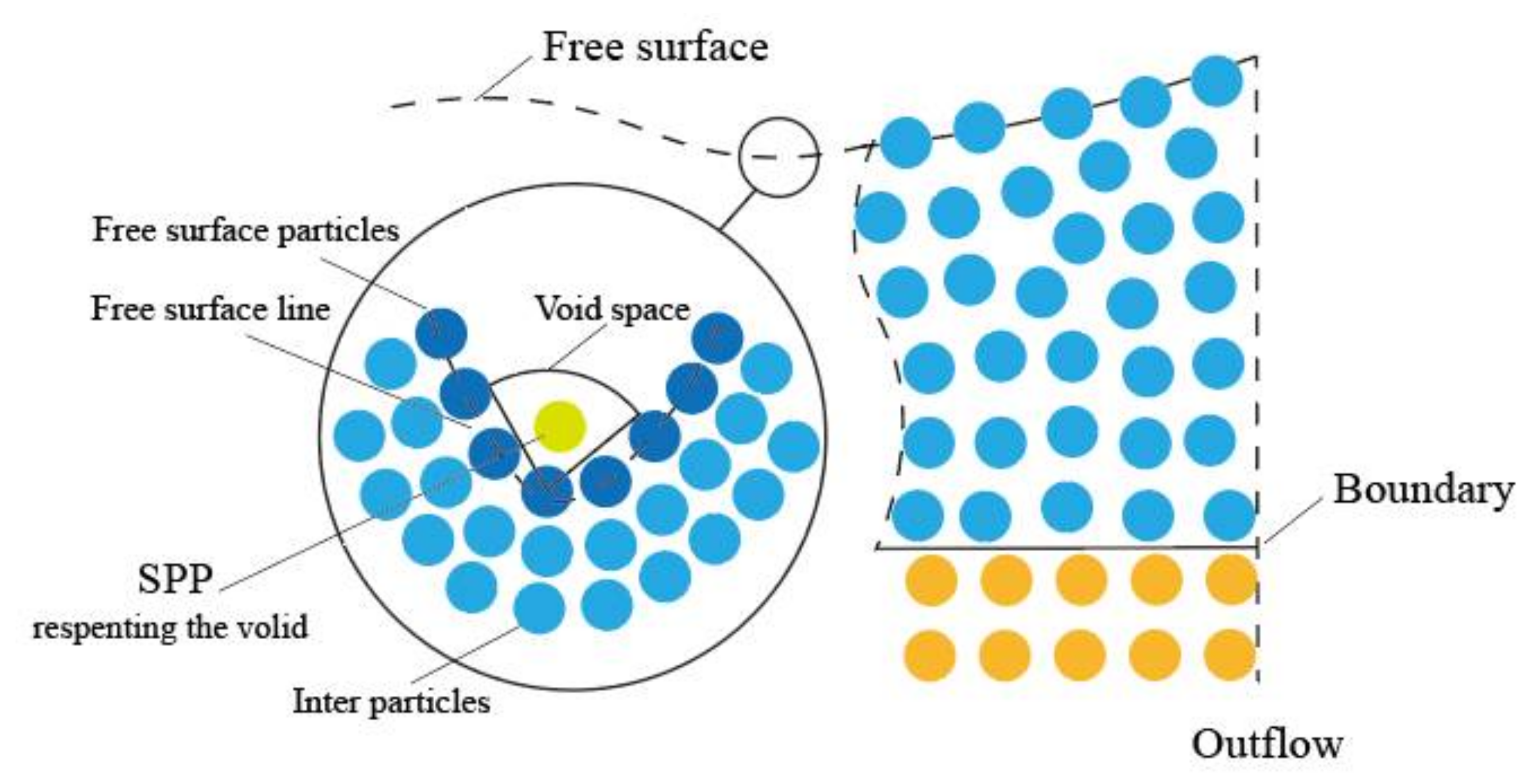

Publisher’s Note: MDPI stays neutral with regard to jurisdictional claims in published maps and institutional affiliations. |
© 2022 by the authors. Licensee MDPI, Basel, Switzerland. This article is an open access article distributed under the terms and conditions of the Creative Commons Attribution (CC BY) license (https://creativecommons.org/licenses/by/4.0/).