Methodology to Assess the Technoeconomic Impacts of the EU Fit for 55 Legislation Package in Relation to Shipping

Abstract

The recent inclusion of shipping in the Fit for 55 legislation package will have large knock-on effects on the industry and consequently on end consumers. The present paper presents an innovative top-down methodology, the MSF455 model, which estimates the new vessel Operational Expenditure (OPEX) as per the provisions of the Fit for 55 package and various scenarios based on carbon tax, penalty allowances, maritime fuel tax and effect. The methodology is presented and tested against six scenarios that are based on Det Norske Veritas’s (DNV) fuel maritime projections. The model illustrates that the distinction between intra-EU and extra-EU penalty allowance creates a large disparity and thus reduction in the competitiveness of goods (produced and transported).

1. Introduction

Maritime transport is important for the trade, and therefore, economies of countries, which makes it a very popular transportation mode. However, shipping companies as well as port operators, as reviewed by Elmi et al. [1] and Bastug et al. [2], are facing many challenges, including disruptions in terms of port congestion, weather conditions, the recent COVID-19 pandemic, and port competitiveness to name a few. The recently proposed “Fit for 55” package adds an additional challenge to shipping, which has an important international dimension as European member states and the European Commission have endorsed it in order to be in line with the Paris Agreement (COP21);p however, it is still under debate. The European Union (EU) wants to be carbon neutral by 2050 and also wants to curb emissions by 55–60% by 2030 to be in line with the 1990 baseline. On 12 December 2019, the European Council and the European Commission established the European Green Deal, which is the key strategy for climate neutrality. Subsequently, on 14 July 2021, the European Commission adopted the “Fit for 55” legislation package aiming to reduce greenhouse gas emissions (GHG) by 55% by 2030 compared to the 1990 baseline [3]. It is noteworthy that many aspects of the “Fit for 55” legislation packages include shipping. Stakeholders in shipping, on the other hand, such as the International Maritime Organization (IMO), are currently discussing the 2050 deep decarbonization targets. The current stance by the IMO is to reduce by at least 50% the GHG emissions compared to 2008 baseline, irrespective of maritime trade growth [4,5].

The main objectives of the “Fit for 55” package can be summarized as [6]: (1) Guarantee environmental integrity and solidarity, (2) strengthen the EU Emissions Trading System (ETS), which now includes shipping, (3) add policies to help with carbon taxation and ensure the implementation of carbon prices (although these are still under debate), and (4) introduce carbon pricing and respective taxation to positively influence end consumers. The relevant Fit for 55 legislation measures that directly affect shipping are: (1) EU ETS, (2) FuelEU Maritime, (3) Revised Energy Taxation Directive (ETD), (4) Revised Renewable Energy Directive (RED) II, (5) EU Maritime Monitoring, Reporting, and Verification (MRV) Regulation, (6) Alternative Fuel Instructive Directive (AFID), and (7) Carbon Border Adjustment Mechanism (CBAM). There are limited studies that investigated the impact of the Fit for 55 legislation package on the shipping industry.

Therefore, an innovative top-down approach and algorithm has been developed to estimate effect of OPEX as part of the measures imposed by “Fit for 55”, which are a CO₂ penalty (inclusion of shipping in EU ETS), fuel maritime tax, effect of imports at intra- and extra-EU level and projections of fuel costs of conventional fossil fuels and alternative green fuels (such as hydrogen, ammonia, methanol, biogas, and bioethanol) as well as bridging fuels such as Liquefied Natural Gas (LNG) and Liquefied Petroleum Gas (LPG). Apart from the reduced GHG emissions, LNG can reduce the amount of SOx emissions, which is particularly important for Sulphur Emission Control Areas (SECA) [7]. The most popular alternative fuels in shipping are examined. Different scenarios will be investigated to determine the effect of OPEX on a per vessel basis and its ability to transport goods and products to EU ports. Note that OPEX includes operating costs of a vessel such as wages, stores, repair and maintenance, and cost of fuel to name a few [8]. The structure of the paper is to provide an oversight of the “Fit for 55” in relation to shipping and size of gross weight handled by EU ports (Section 2). The methodology of the proposed algorithm to estimate the new OPEX by considering the Fit for 55 provisions (Section 3) is presented. A detailed results and discussion in relation to various scenarios is presented in Section 4 to illustrate the universal nature of the proposed methodology considering all provisions of the “Fit for 55”. Finally, the main conclusions and future work is discussed in Section 5.

2. Background

2.1. Importance of Vessel Operating Expenditure (OPEX)

Stopford [9] (p. 544) defined OPEX as the operational costs of a vessel, which include the “day-to-day” costs of operating and maintaining a vessel. These can be administration, crew wages and expenses, fuel costs, maintenance and repairs, lubricants, insurance, stores, and spares to name a few. In addition, some of the aforementioned items may have more economies scales more than others. For example, administration, stores, and wages do not significantly increase, whereas insurance and maintenance may increase with vessel size, which is related to the transport capacity of a vessel [9] (p. 544). The percentage of fuel cost to OPEX is the most significant cost, which is more significant than crew wages [10,11]. Therefore, in this respect, and similarly to other industries, shipping is affected by the volatility of fuel prices [10].

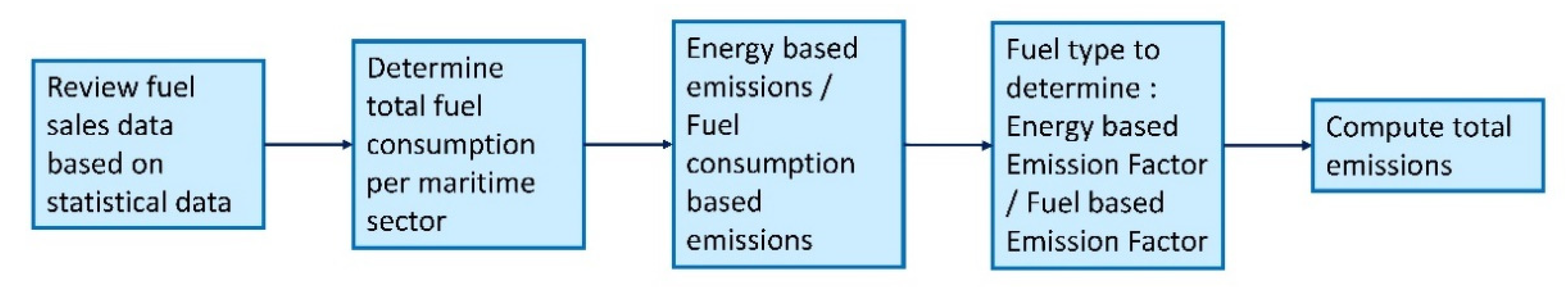
2.2. Various Approaches to Determine Emissions from Shipping

Common models to determine emissions are either in a macro-economic scope (top-down) or an engineering scope (bottom-up). Typically, a top-down approach focuses on market interactions within the whole economy and has little technological detail, while a bottom-up approach focuses on the sustainability of individual energy technologies and their relative costs. For example, the 4th IMO GHG study report recommends using yearly fuel sales statistics [12]. Methodologies for the assessment of ship emissions span from a full top-down to a full bottom-up approach [13].

Bottom-up approaches estimate emissions from shipping by utilizing Autonomous Identification System (AIS) data, where vessel characteristics are provided by a vessel characteristics provider, which are installed propulsive power, installed auxiliary power, reference speed, reference draught, and fuel types to name a few, as well as weather conditions. Note that AIS data track individual ship movements and operational modes, which are based in Very High Frequency (VHF) radio transmissions (either satellite or terrestrial transmissions) and fleet activity [12,14,15]. More details regarding the bottom-up methodology can be found in the 4th IMO GHG study report [12].

The top-down (fuel-based) approach is based on the combination of data on marine fuel sales (quantities and types) or cargo statistics [16] and fuel-related emission factors [17,18]. The major limitation of top-down approaches is the inability to track ship movements in real time, which can lead to uncertainties and inconsistencies in the calculation of emissions [17,19]. The fuel-based approach is commonly used by several countries to prepare domestic and international emission inventories [20]. This approach is used when it is not possible to obtain refined data traffic information; nonetheless, an energy-based approach can be used to estimate GHG emissions [12]. Figure 1 describes the general top-down methodology.

Other methodologies combine the top-down and bottom-up approaches to form hybrid methodologies. For example, a bottom-up approach is used to estimate the total emissions with a top-down approach for geographic characterization. On the other hand, AIS data (as a bottom-up approach) can be used to determine the geographic characterization of vessels combined with a top-down approach to determine total emissions.

In this work, a top-down approach is used, but rather than looking at fuel sales statistics, fuel consumption is estimated and linked to the OPEX of a particular vessel. OPEX values and their corresponding percentage in fuel costs have been obtained from the available literature and are provided in

Table 1. OPEX with corresponding percentage of fuel cost to OPEX. Data processed from [21,22,23]. * Interpolated data by assuming a linear relationship.

Ship Type	DWT/TEU	OPEX ($)	% Fuel Cost to OPEX
Bulker (in DWT)	Mini—Handysize (3000–40,000)	21,497	47%
	Hadymax & Supramax (40,000–60,000) *	24,930	45%
	Panamax (60,000–80,000)	28,363	43%
Container (in TEU)	Small feeder (500–700)	16,470	54%
	Feeder (1000–2000)	26,456	54%
	Feedermax (2000–3000) *	35,398	50%
	Panamax (5000–6000)	53,283	46%
	Post-Panamax (8000–9000)	68,776	42%
	Post-Panamax (10,000–12,000)	84,217	44%
Pure car carrier (in DWT)	0–10,000	68,776	42%
	10,000–20,000	84,217	44%
	20,000–30,000	100,000	45%
	30,000–40,000	116,000	46%
Ro-Ro (in DWT)	1000–6000	60,000	66%
Tanker (in DWT)	General Purpose Tanker (10,000–25,000) *	27,000	30%
	Medium Range Tanker (25,000–45,000)	30,953	30%
	Large Range 1; LR1 (45,000–80,000)	36,636	30%
	Large Range 2; LR2 (80,000–160,000)	53,838	36%

. These values were used in the MSF455 model, but can equally be modified according to end-user, technological, and/or market developments.

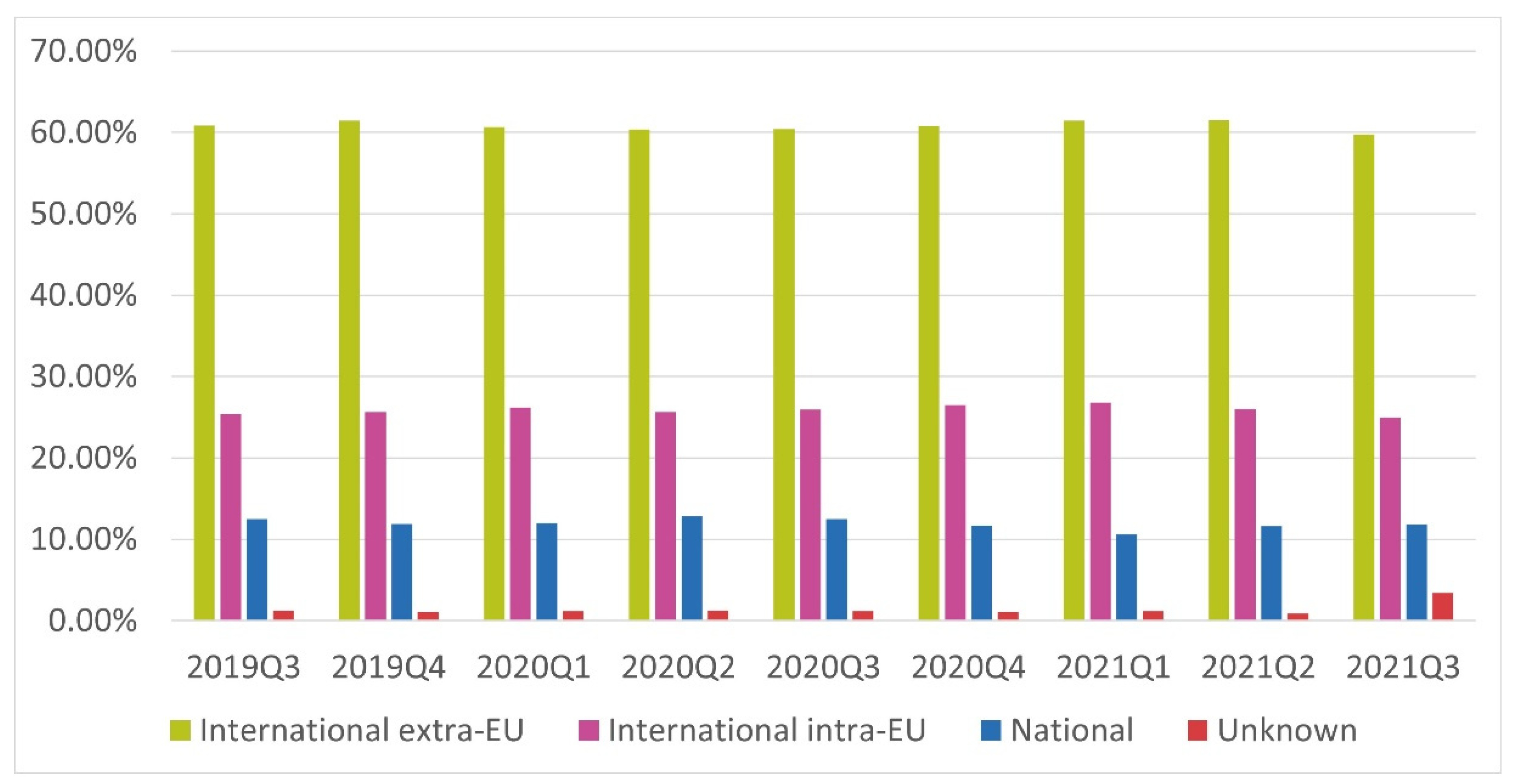
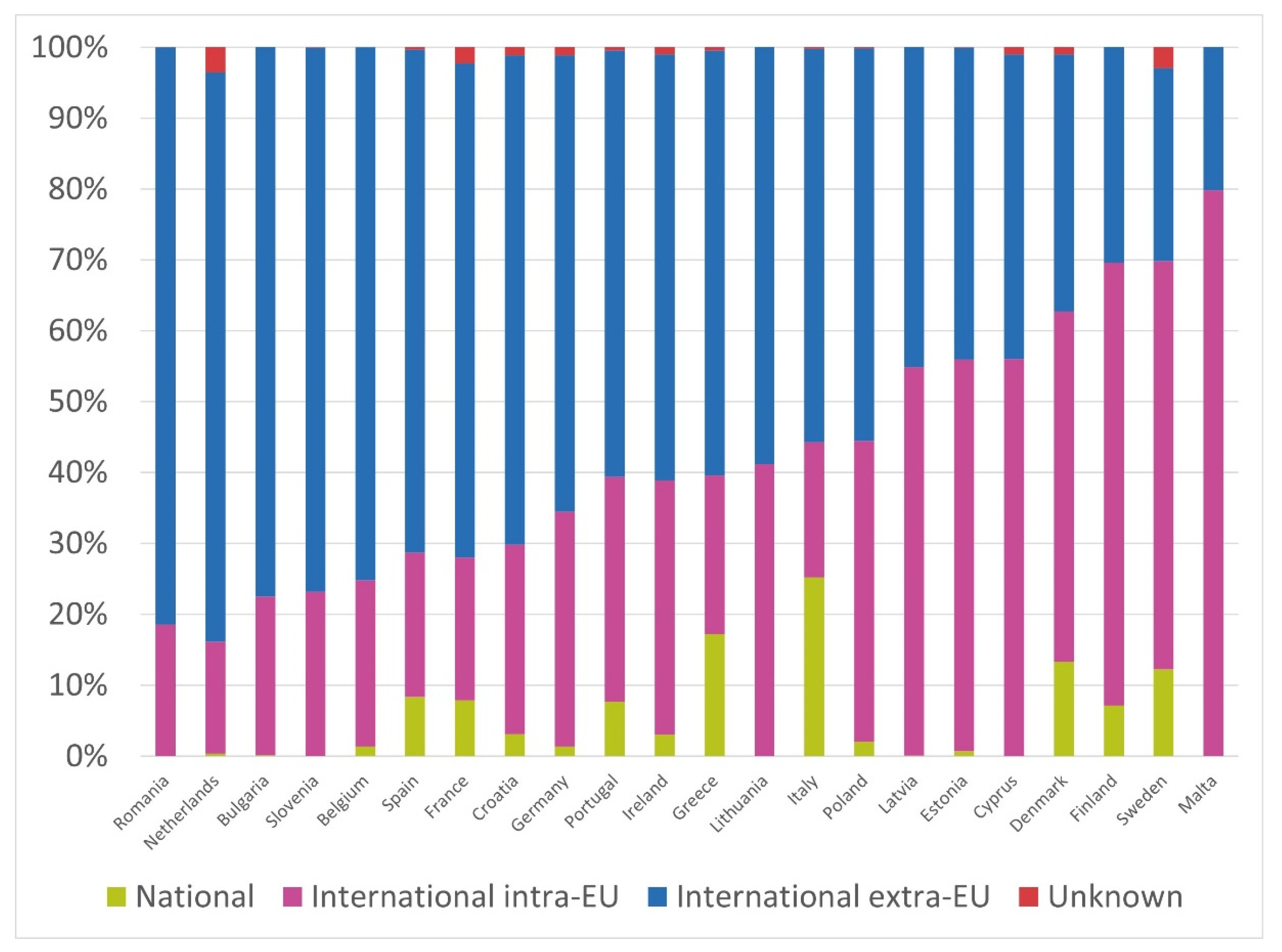
2.3. Intra-EU Versus Extra-EU Imports/Exports Handled by EU Ports

According to Eurostat [24], ~60% of the goods handled by main EU ports are international extra-EU compared to ~25% as international intra-EU (see Figure 2). CBAM sets a factor γ = 1.0 for intra-EU imports/exports, and γ = 0.5 for extra-EU imports/exports to be imposed on a pre-agreed CO₂ EUR/tonne tariff. However, the distinction between intra-EU and extra-EU ports constitutes that those goods produced and transported within the EU (intra-EU) will be less competitive as opposed to similar goods produced and transported outside the EU (extra-EU). This is also evidenced by looking at seaborne transport of freight between main ports in the reporting country and their partner ports.

Figure 3 illustrates the seaborne transport by freight between main ports in the reporting country and their partner ports grouped by main geographical areas in 2020 [25] and highlights the large disparity on a per EU country considering the effect between intra-EU and extra-EU imports/exports. Note that countries with long shorelines or with a large number of islands, such as Italy, Greece, and Norway, have a high national seaborne transport. Countries with high intra-EU imports/exports, such as Malta, Cyprus, Finland, Sweden, Estonia, Latvia, and Denmark, have high intra-EU imports/exports because their main partners are within the EU. On the other hand, countries such as Romania, the Netherlands, Bulgaria, Slovenia, Belgium, Spain, France, and Croatia have high extra-EU import/export percentages due to their geographic position [25].

2.4. Market Based Measures

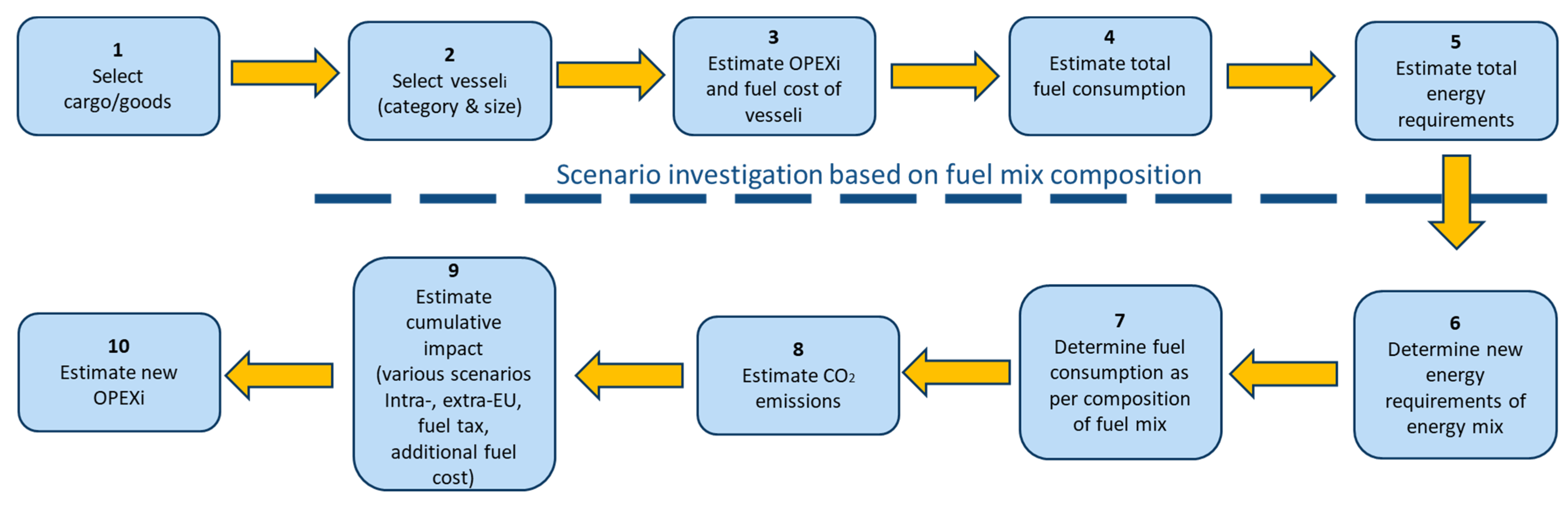
The shipping industry is regulated by the International Maritime Organization (IMO); hence, for any relevant measures and regulations, the impact on shipping will also need to be considered. Market-based measures (MBMs) is not a new concept in shipping, as it has been under debate since 2006 in the Marine Environment Protection Committee (see MEPC56 [26]), with little progression up until MEPC65 [27]. Similar to the Fit for 55 package, the MBMs are based on economic indicators and/or tax levies [28].

An overview of MBMs proposal is reviewed and well explained by Psaraftis et. al. [29]. It is noteworthy that progress on MBMs was halted due to disagreement on the direction of relevant stakeholders [28]. On the other hand, under the umbrella of the European Green Deal [29,30], shipping will be included under the EU ETS, imposing a CO₂ EUR/tonne tariff. An agreement between EU member states on the CO₂ EUR/tonne tariff up until 2030 is yet to be finalized and is currently under debate.

We believe that MBMs will act as an incentive for all relevant stakeholders such as governments, industry, and research institutions to offer technological solutions via innovative new and radical technologies or apply existing technologies to address the current climate change challenges in shipping that will be in line with existing and upcoming measures, policies, and legislations.

3. Methodology

Figure 4 depicts the MSF455 algorithm, which assesses OPEX based on CO₂ penalties (predicted and current), fuel mixture, cost of fuel (predicted and current), percentage of taxation of maritime bunker fuels (currently non-taxable), and estimated impact on final value (percentage increase) on products arriving at EU ports considering intra- and extra-EU imports.

• Step 1: Select the cargo/goods to be transported, i.e., imported/exported based on value i, where subscript i indicates vessel type.
• Step 2: Based on the category of goods transported, identify the appropriate vessel (e.g., bulker for food, beverages, durable and semi durable items, RoRo for cars and equipment, container for a variety of goods, and tanker for fuels and lubricants) based on vessel_i.
• Step 3: Estimate the OPEX_i of vessel_i. The OPEX is estimated from various sources [21,22,23]. However, the algorithm can adjust to varying OPEX values accordingly to market trends.
• Step 4: Estimate fuel consumption via:

$$F{C}_i=\frac{OPE{X}_i\ast f}{C_{2022}}$$

(1)

where FC_i is the fuel consumption of the fuel mix in kg per vessel_i, f is the % of fuel cost to OPEX_i, and C₂₀₂₂ is the fuel cost per barrel of oil equivalent (boe) for 2022. See

Table 2. International oil fuel prices assumptions based on the REF2020 scenario [31]. Values are linearly interpolated on a per-year basis.

In USD/boe	2020	2022	2023	2024	2025	2026	2027	2028	2029	2030
Oil	39.8	47.84	51.86	55.88	59.90	63.94	67.98	72.02	76.06	80.10

for USD/boe based on the REF2020 scenario [31]. It should be noted that the REF2020 scenario was used to develop the Fit for 55 package. However, the current oil prices are not in agreement with the REF2020 scenario because of the geopolitical situation in Europe (current Ukraine war) and the effects of the COVID-19 pandemic.

Step 5: Estimate the total energy requirements of vessel_i:

$$F{E}_i=F{C}_i\ast LH{V}_{HFO}$$

(2)

where $F{E}_i$ is the total energy requirements per vessel and $LH{V}_{HFO}$ is the Latent Heating Value of HFO (40 MJ/kg).

• Step 6: The new energy requirements are determined based on the new energy composition; these are user input requirements:

$$F{E}_{ij}=F{E}_i{\eta }_{ij}{\alpha }_{ij}$$

(3)

where subscript j indicates fuel type and ${\eta }_{ij}$ is the change in total energy requirements due to switching to a different fuel (change in combustion efficiency). In this work, alternative fuels are assumed to improve combustion efficiencies, with efficiencies of 98%, as opposed to their fossil fuel counterparts, although the change in improvement depends on several factors, such as fuel composition, type of engine, and type of injection to name a few. ${\alpha }_{ij}$ is the percentage of fuel j of vessel i.

• Step 7: Determine fuel mass i of fuel mix based on new energy requirements of vessel i:

$$F{C}_{ij}=F{E}_{ij}/LH{V}_j$$

(4)

where FC_ij is the fuel consumption of vessel i and fuel type j. LHV_j is the latent heat value of fuel type j.

• Step 8: Estimate total CO₂ emissions of new fuel mix of vessel i:

$$C{O}_{2,i}={\displaystyle \sum }_j\left(F{C}_{ij}\ast E{F}_j\right)$$

(5)

where EF_j is the fuel-based emission factor of fuel j. Note that emission factor for other GHG, such as methane, can be included in the methodology from the 4th IMO GHG study [11].

• Step 9: Estimate the cumulative impact based on scenarios for CO₂ tax, intra- and extra-EU, fuel tax, and additional fuel cost up to 2050:

$$taxplu{s}_{ik}=C{O}_{2}ta{x}_{ik}+fuelta{x}_{ik}+additionalfuelcos{t}_{ik}$$

(6)

where $taxplu{s}_{ik}$ is the added tax per year k on vessel i. It is composed of $C{O}_{2}ta{x}_{ik}$ which is the CO₂ penalty defined as:

$$C{O}_{2}ta{x}_{ik}=\gamma {\delta }_k{\epsilon }_{k}C{O}_{2,i}$$

(7)

where γ = 1.0 for intra-EU imports/exports, γ = 0.5 for extra-EU imports/exports, ${\delta }_k$ is the CO₂ penalty in EUR/tonne for year k, and ${\epsilon }_k$ is the carbon penalty allowance as per CBAM until 2026 (see

Table 3. Penalty allowance until 2026 as predicted by the Carbon Border Adjustment Mechanism.

Year	2023	2024	2025	2026	2027	2028	2029	2030
ε (%)	20%	45%	70%	100%	100%	100%	100%	100%

).

$fuelta{x}_{ik}$ is the fuel tax on maritime bunker fuel defined as:

$$fuelta{x}_{ik}={\displaystyle \sum }_j{\theta }_{kj}\ast F{E}_{ij}\ast C_{kj}$$

(8)

where θ_kj is the maritime tax for year k and fuel type j and C_kj is the cost of fuel j for year k per MJ. Note that θ_kj is only applied to intra-EU routes as it is expected vessel route optimization will be involve avoiding ports with potential maritime tax implications.

$additionalfuelcos{t}_{ik}$ is the additional fuel cost of fuel j based on projects and reference year (2022):

$$additionalfuelcos{t}_{ik}={\displaystyle \sum }_{j}F{E}_{ij}\left(C_{jk}-C_{j2022}\right)$$

(9)

• Step 10: Estimate the cumulative impact based on scenarios for CO₂ tax, intra- and extra-EU, fuel tax, and additional fuel cost up to 2030:

$${\pi }_{ik}=taxplu{s}_{ik}/OPE{X}_i$$

(10)

3.1. Fuel Parameters

Table 4. Fuel parameters that were used in the scenarios of this work.

Fuel Mix	HFO	MGO	Green H2	Green NH3	Green Methanol	Biogas	LNG	Advanced Biodiesel
Latent Heat Value (MJ/kg)	40.00	43.00	120.00	18.60	19.90	50.00	50.00	38.00
Emission factor (-)	3.114	3.206	0.000	0.000	0.000	0.000	2.755	0.000
Change in energy requirements (${\eta }_{ij}$) (%)	100.00	100.00	98.00	98.00	98.00	98.00	98.00	98.00

lists possible fuel parameters, which includes alternative green fuels, such as hydrogen, ammonia, biogas, methanol, and advanced biodiesel, bridging fuels, such as LNG, and the conventional fossil fuels that are currently used in shipping, such as heavy fuel oil (HFO) and marine gasoil (MGO).

3.2. Scenarios Based on Fuel Mix, Fuel Tax, CO₂ Penalty, and Cost of Fuel until 2030

The scenarios presented in

Table 5. Scenario A: BAU DNV fuel maritime mix at 2018 and Scenario B: DNV fuel maritime mix at 2030, fuel mix obtained from [32,33]. ** Very small contribution, and therefore, considered zero. Note that “electricity from grid” is ignored in the energy mix; hence, mix is readjusted. Scenarios F1 and F2 refer to fuel tax scenarios based on the relevant fuel maritime mix.

Fuel Mix	HFO	MGO	Green H2	Green NH3	Green Methanol	Biogas	LNG	Advanced Biodiesel
Scenario A—BAU
Composition (%)	77.81	19.76	0.00	0.00	0.00	0.00	2.43	0.00
Fuel tax (%)	0.00	0.00	0.00	0.00	0.00	0.00	0.00	0.00
Scenario AF1
Composition (%)	77.81	19.76	0.00	0.00	0.00	0.00	2.43	0.00
Fuel tax (%)	10.00	10.00	0.00	0.00	0.00	0.00	0.00	0.00
Scenario AF2
Composition (%)	77.81	19.76	0.00	0.00	0.00	0.00	2.43	0.00
Fuel tax (%)	20.00	20.00	0.00	0.00	0.00	0.00	0.00	0.00
Scenario B
Composition (%)	17.32	44.29	0.00	0.56	0.00	0.00 **	35.95	1.88
Fuel tax (%)	0.00	0.00	0.00	0.00	0.00	0.00	0.00	0.00
Scenario BF1
Composition (%)	17.32	44.29	0.00	0.56	0.00	0.00 **	35.95	1.88
Fuel tax (%)	10.00	10.00	0.00	0.00	0.00	0.00	0.00	0.00
Scenario BF2
Composition (%)	17.32	44.29	0.00	0.56	0.00	0.00 **	35.95	1.88
Fuel tax (%)	20.00	20.00	0.00	0.00	0.00	0.00	0.00	0.00

are based on the DNV projections regarding the maritime fuel mix up to 2030 [32]. Note that the purpose is not to evaluate the scenarios and their validity but assess the implementation of the algorithm and methodology of MSF455. This is because the methodology will be heavily dependent on input parameters that depend on market conditions, the final decision on Fit for 55, the advancement and maturity of technologies, availability, supply, and demand of fuels, and even specific allowances on a per-country basis.

Table 5 lists six different scenarios: scenario A is the Business as Usual (BAU) scenario, where the maritime fuel mix of 2018 as presented by the Energy Transition Outlook by DNV [32] is assumed to be the same up until 2030. Scenarios AF1 and AF2 apply a fuel tax on HFO and MGO with BAU fuel composition. Scenario B is a what-if scenario with the fuel maritime mix at 2030 as projected by DNV [32] applied to 2023 and onwards. Note that fuel composition in the presented scenarios is considered constant in time; however, the MSF455 model can also accept fuel composition as temporal functions. This will allow additional flexibility to end-users who may want to investigate the impact of fuel maritime mix variation in time, as for example presented by DNV [32]. Scenarios BF1 and BF2 apply a fuel maritime tax on HFO and MGO on scenario B.

Table 6. CO₂ penalty and fuel cost scenarios with projections up to 2030 (and beyond) as per the proposed Fit for 55 legislation package. A linear distribution has been used on a per year basis. In this work, values of EUR/metric quantity have been obtained from the available literature and converted to EUR/MJ. Where projections were needed, and unavailable linear relationships were assumed. Fuel costs were obtained from the following references [31,34,35,36,37]. For biodiesel the cost fluctuates based on location and feedstock end price, but was assumed to be as reported in [37] with a constant price up to 2030.

Year	2022	2023	2024	2025	2026	2027	2028	2029	2030
δ (EUR/tonne)	-	42.50	50.71	58.93	67.14	75.36	83.57	91.70	100.00
HFO (EUR/MJ)	0.008	0.009	0.010	0.010	0.011	0.012	0.012	0.013	0.014
MGO (EUR/MJ)	0.008	0.009	0.010	0.010	0.011	0.012	0.012	0.013	0.014
Green H2 (EUR/MJ)	0.031	0.030	0.029	0.028	0.027	0.026	0.025	0.024	0.023
Green NH3 (EUR/MJ)	0.031	0.030	0.029	0.028	0.027	0.026	0.025	0.024	0.023
Green Methanol (EUR/MJ)	0.042	0.039	0.037	0.034	0.032	0.030	0.029	0.026	0.022
Biogas (EUR/MJ)	0.018	0.016	0.014	0.012	0.011	0.009	0.007	0.005	0.004
LNG (EUR/MJ)	0.004	0.009	0.013	0.018	0.022	0.026	0.031	0.035	0.040
Advanced biodiesel (EUR/MJ)	0.026	0.026	0.026	0.026	0.026	0.026	0.026	0.026	0.026

imposes various carbon penalties, δ (EUR/tonne) and an estimated cost of fuel (EUR/MJ) as gathered from the available literature [31,34,35,36,37]. Note that these are input and can be modified as required depending on penalty allowance, final decision of carbon penalties, technological maturity, and availability of alternative fuels, which can affect the estimated cost of fuel.

4. Results and Discussion

The presented methodology was applied and presented to the Ministry of Finance and Ministry of Energy, Commerce, and Industry of the Republic of Cyprus under an agreed Memorandum of Understanding [38]. The methodology was applied to the case of Cyprus and various scenarios related to the energy balance (as given by Eurostat [39]) of the country were investigated in relation to the effect of the “Fit for 55” package. This section will demonstrate the MSF455 methodology based on the aforementioned six scenarios. The MSF455 methodology evaluates the effect of OPEX on a per-vessel basis depending on the Fit for 55 provisions. However, it does not link the effect of changing OPEX to supply and demand and Gross Domestic Product (GDP) on a per-EU member state basis, as similarly done by the PRIMES-Maritime transport model, which uses a bottom-up methodology [40,41]. Note that both MSF455 and the PRIMES-Maritime transport model project the energy consumption, and thus, fuel consumption on a per-vessel basis, which enable the estimation of GHG emissions. In addition, the effect on basic commodities, such as imported fuel, will be examined for the Cyprus case study.

Transport & Environment [42] examined the impact of FuelEU Maritime, EU ETS and other relevant legislations with scenarios that include the uptake of e-fuels, including ambitious and less ambitious energy efficiency measures. Based on their scenarios, they have concluded that green ammonia “appears to be the cheapest fuel to decarbonise EU-related shipping”. In the same study, it is suggested that green liquid hydrogen will catch up by 2050. The International Monetary Fund (IMF) has performed various scenarios on carbon tax, such as “$75 per tonne of CO₂ in 2030 ($240 per tonne of bunker fuel), and $150 per tonne in 2040” to act as an incentive to reduce maritime emissions [43]. In their study, the IMF suggests that carbon taxes are a promising way to achieve emissions reductions in a promising way.

However, such studies do not mention the impact on intra- and extra-EU routes with relevance to three additional costs, herein called taxplus (Equation (6)), which are fuel maritime tax, additional fuel cost, and CO₂ penalties. These are further elaborated in the next subsections.

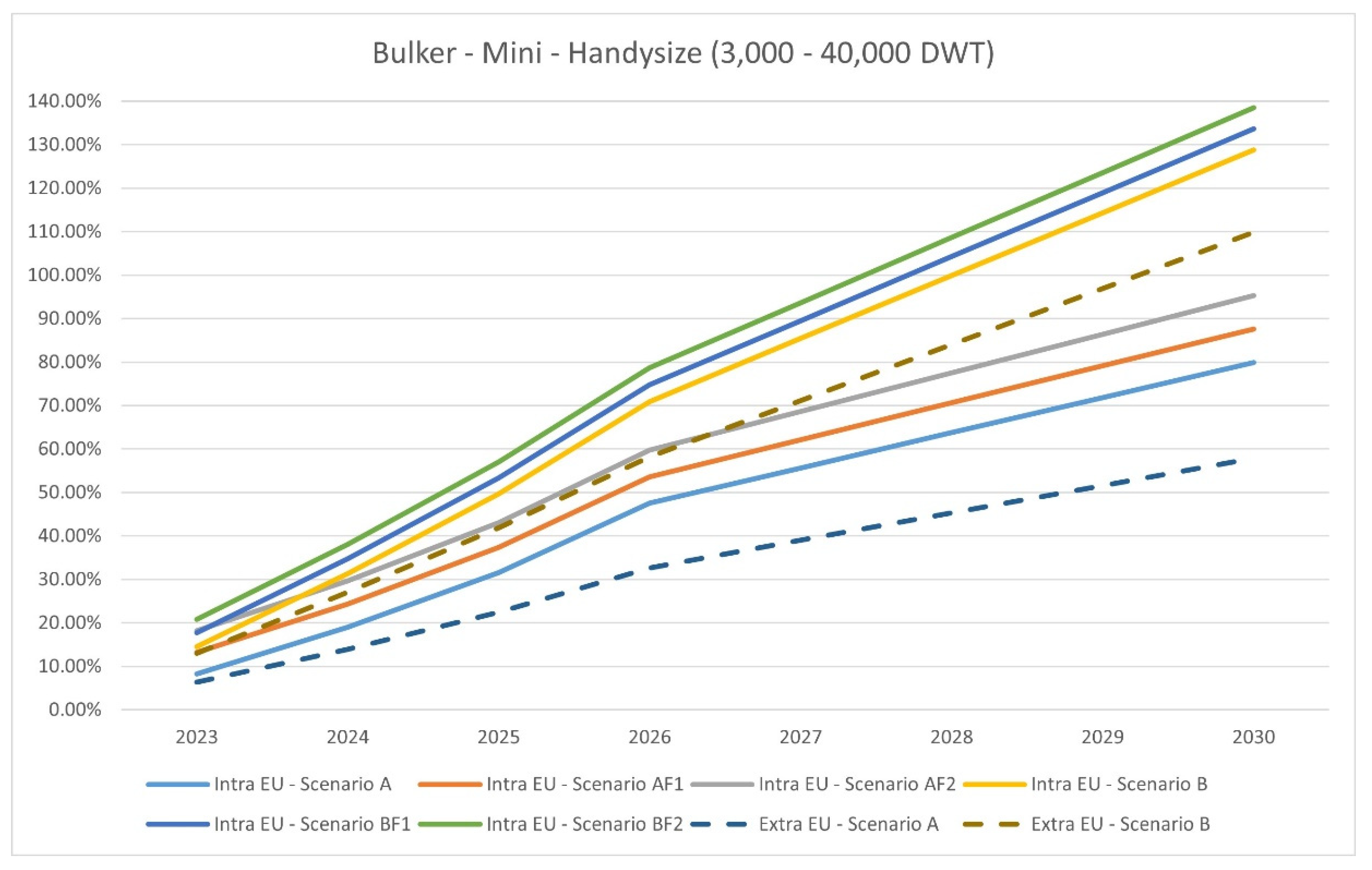
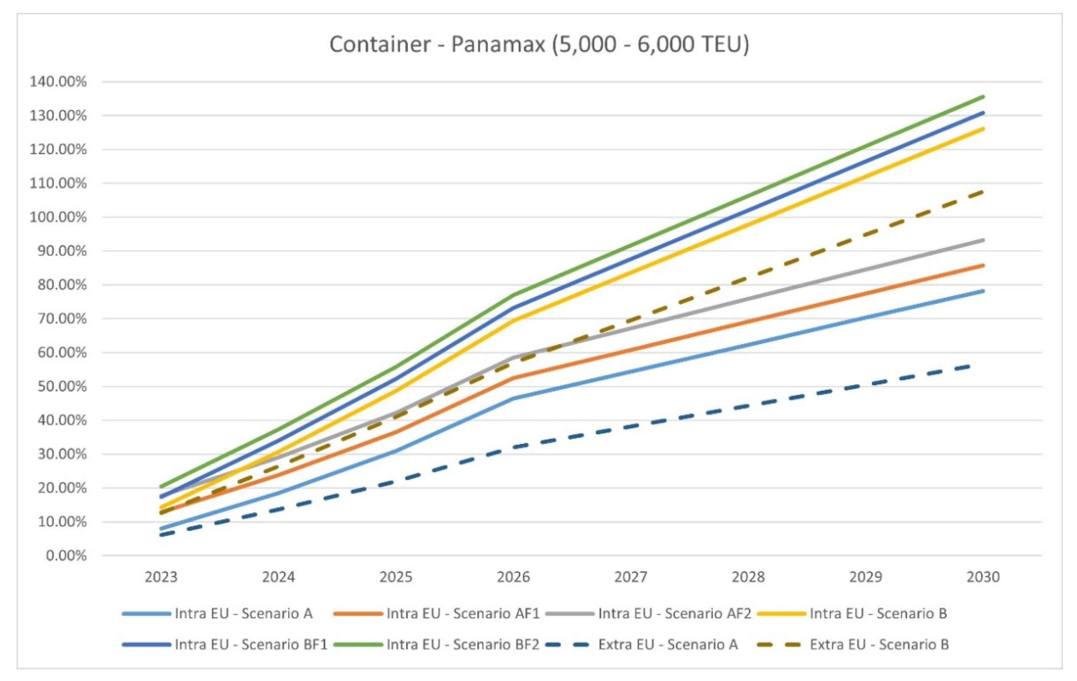
4.1. Effect of OPEX Due to Intra-EU and Extra-EU and Fuel Maritime Tax

Figure 5 presents the effect on OPEX of bulker vessels of size Mini-Handysize (size range 3000–40,000 DWT) on the various scenarios. Figure 6 presents the effect on OPEX of container vessels of size Panamax (size range 5000–6000 TEU) on the various scenarios. Figure 7 presents the effect on OPEX of tanker vessels of Large Range 1; LR1 (size range 45,000–80,000 DWT) on the various scenarios. The figures also compare intra-EU and extra-EU scenarios. The Revised ETD proposes a minimum of EUR0.90/GJ tax on bunker fuels for intra-EU routes in 2023 [44], thus making them less competitive compared to extra-EU routes. However, currently fuel maritime tax is exempted and currently under debate if it is to be included in the Fit for 55 legislation package [45].

It is notable, and as illustrated by Figure 5, Figure 6 and Figure 7, that in any fuel tax scenario, the effect on OPEX of extra-EU imports/exports is significantly less than the corresponding intra-EU scenario. This highlights the earlier point that the Fit for 55 provisions would constitute that goods transported within EU ports are less competitive than goods transported from/to non-EU ports.

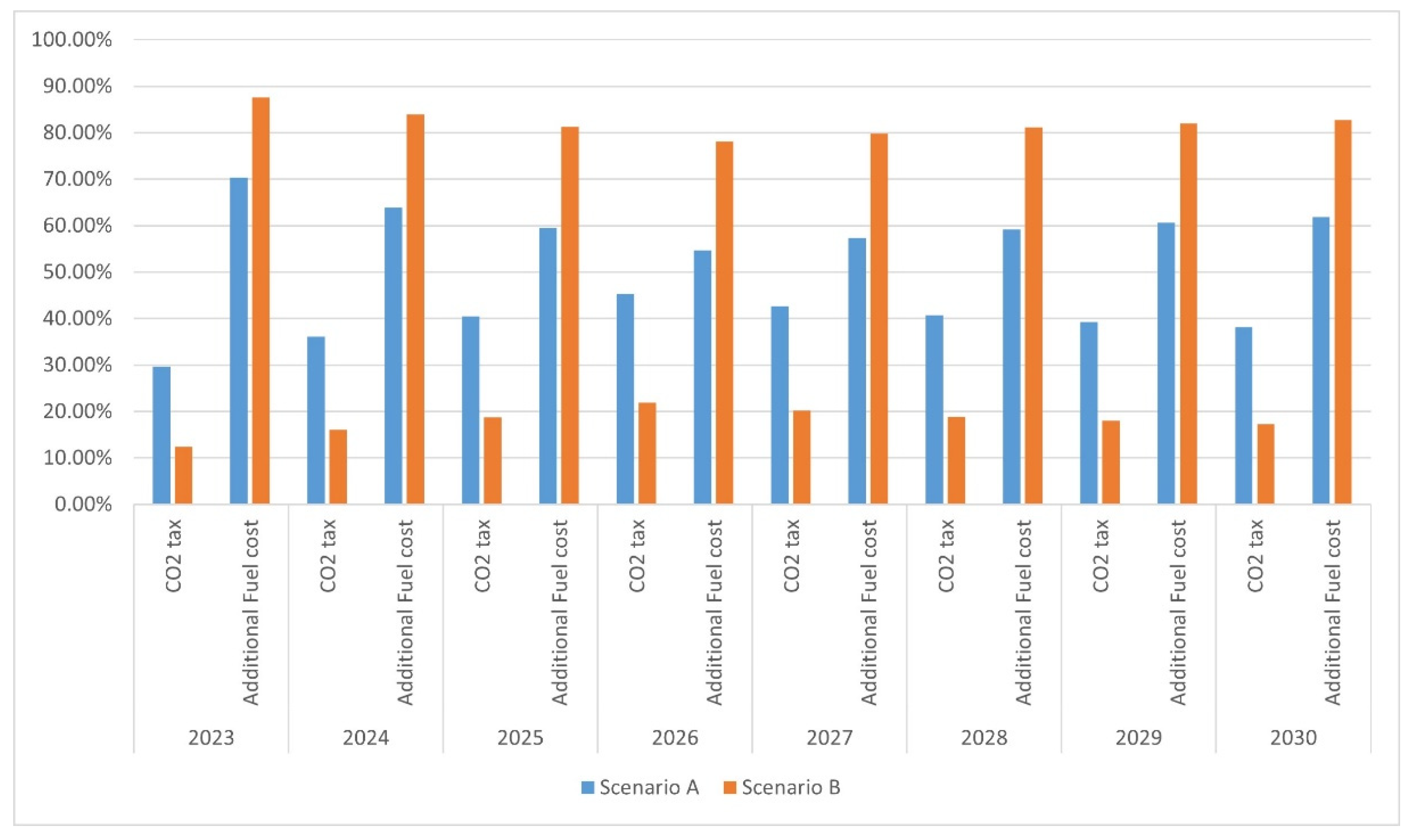
4.2. Breakdown of Taxplus

Taxplus is divided into CO₂ tax (EUR/tonne), additional fuel cost, and fuel tax, as defined by Equations (6)–(9). Note that for extra-EU routes, taxplus is not influenced by fuel tax, as it is envisioned that the vessel route will be optimized in such a way to avoid fuel tax, i.e., refueling or bunkering at non-EU ports. Thus, scenarios AF1, AF2, BF1, and BF2 are irrelevant for extra-EU routes.

Figure 8 shows the breakdown of taxplus for intra-EU routes based on the presented scenarios of Table 5. Figure 9 shows the breakdown of taxplus for extra-EU routes based on scenarios A and B presented in Table 5. The model predicts that irrespective of intra- versus extra-EU, the most important parameter that affects the new OPEX of a vessel is the additional fuel cost. However, as the CO₂ penalty is still under debate, this proportion will change if higher tariffs than those presented in Table 6 are assumed. Of course, the assumptions on the fuel cost presented in Table 6 will have a significant impact.

5. Conclusions and Future Work

In this study, an innovative top-down methodology, the MSF455 model, was presented. The methodology of the proposed model estimates the new OPEX of a vessel by taking into account the Fit for 55 provisions based on several scenarios. In this work, the scenarios have been obtained from DNV’s Energy Transition Outlook of the current maritime fuel mix (2018) as business as usual and projected maritime fuel mix by 2030. Fuel tax, cost of fuel, and CO₂ penalties were based on hypothetical scenarios, since these are still under debate. The methodology presented can be used to evaluate any possible scenario under debate by the relevant stakeholders.

The model has limitations, because it is not related to a macro-economic model; therefore, it is planned to be extended to include the effect on GDP and other economy-related KPIs per EU member state and the effect on supply and demand due to different vessel OPEX values. It is expected that the estimated increase in OPEX will significantly affect (1) the overall demand for goods and (2) the competitiveness of the EU Member States’ economies. It is also expected that the Fit for 55 provisions will not equally affect the EU citizens’ and the EU countries’ economies. It should be noted that the methodology and algorithm can be applied to any EU country to include shipping transportation at EU ports and could be further extended to include intermodal transportation. The proposed methodology can be also utilized in order to detect weaknesses and vulnerabilities and assess the impact of a variety (and mix) of measures to be taken.

References

1. Elmi, Z.; Singh, P.; Meriga, V.K.; Goniewicz, K.; Borowska-Stefańska, M.; Wiśniewski, S.; Dulebenets, M.A. Uncertainties in Liner Shipping and Ship Schedule Recovery: A State-of-the-Art Review. J. Mar. Sci. Eng. 2022, 10, 563. [Google Scholar] [CrossRef]
2. Baştuğ, S.; Haralambides, H.; Esmer, S.; Eminoğlu, E. Port competitiveness: Do container terminal operators and liner shipping companies see eye to eye? Mar. Policy 2021, 135, 104866. [Google Scholar] [CrossRef]
3. European Commission. 2030 Climate & Energy Framework. 2021. Available online: https://ec.europa.eu/clima/eu-action/climate-strategies-targets/2030-climate-energy-framework_en (accessed on 14 June 2022).
4. IMO. UN Body Adopts Climate Change Strategy for Shipping. 13 April 2018. Available online: https://www.imo.org/en/MediaCentre/PressBriefings/Pages/06GHGinitialstrategy.aspx (accessed on 14 June 2022).
5. ECSA. Position Paper: A Green Deal for the European Shipping Industry; European Community Shipowners’ Association: Brussels, Belgium, 2020. [Google Scholar]
6. KPMG. The European Green Deal & Fit for 55. 2022. Available online: https://home.kpmg/xx/en/home/insights/2021/11/the-european-green-deal-and-fit-for-55.html (accessed on 14 June 2022).
7. Sharma, N.R.; Dimitrios, D.; Olcer, A.I.; Nikitakos, N. LNG a clean fuel—The underlying potential to improve thermal efficiency. J. Mar. Eng. Technol. 2022, 21, 111–124. [Google Scholar] [CrossRef]
8. Tsitsoni, D. Revenue and Operating Cost Analysis in the Tanker Sector. Master’s Thesis, Department of Maritime Studies, University of Piraeus, Piraeus, Greece, 2021. [Google Scholar]
9. Stopford, M. Maritime Economics, 3rd ed.; Routledge: London, UK, 2009. [Google Scholar]
10. Bialystocki, N.; Konovessis, D. On the estimation of ship’s fuel consumption and speed curve: A statistical approach. J. Ocean Eng. Sci. 2016, 1, 157–166. [Google Scholar] [CrossRef] [Green Version]
11. Wijnolst, N.; Wergeland, T.; Levander, K. Shipping Innovation; IOS Press: Amsterdam, The Netherlands, 2009. [Google Scholar]
12. Faber, J.; Hanayama, S.; Zhang, S.; Pereda, P.; Comer, B.; Hauerhof, E.; van der Loeff, W.S.; Zhang, H.; Kosaka, M.; Adachi, J.-M.; et al. Fourth IMO Greenhouse Gas Study; International Maritime Organization: London, UK, 2020. [Google Scholar]
13. Toscano, D.; Murena, F. Atmospheric ship emissions in ports: A review. Correlation with data of ship traffic. Atmos. Environ. X 2019, 4, 100050. [Google Scholar] [CrossRef]
14. Tichavska, M.; Tovar, B. Port-city exhaust emission model: An application to cruise and ferry operations in Las Palmas Port. Transp. Res. Part A Policy Pract. 2015, 78, 347–360. [Google Scholar] [CrossRef]
15. Jalkanen, J.-P.; Brink, A.; Kalli, J.; Pettersson, H.; Kukkonen, J.; Stipa, T. A modelling system for the exhaust emissions of marine traffic and its application in the Baltic Sea area. Atmos. Chem. Phys. 2009, 9, 9209–9223. [Google Scholar] [CrossRef] [Green Version]
16. Schrooten, L.; De Vlieger, I.; Panis, L.I.; Chiffi, C.; Pastori, E. Emissions of maritime transport: A European reference system. Sci. Total Environ. 2009, 408, 318–323. [Google Scholar] [CrossRef] [PubMed]
17. Song, S.K.; Shon, Z.-H. Current and future emission estimates of exhaust gases and particles from shipping at the largest port in Korea. Environ. Sci. Pollut. Res. 2014, 21, 6612–6622. [Google Scholar] [CrossRef] [PubMed]
18. Nunes, R.A.O.; Alvim-Ferraz, M.C.M.; Martins, F.G.; Sousa, S.I.V. The activity-based methodology to assess ship emissions—A review. Environ. Pollut. 2017, 231, 87–103. [Google Scholar] [CrossRef]
19. Woo, D.; Im, N. Spatial Analysis of the Ship Gas Emission Inventory in the Port of Busan Using Bottom-Up Approach Based on AIS Data. J. Mar. Sci. Eng. 2021, 9, 1457. [Google Scholar] [CrossRef]
20. European Environmental Agency. Environmental Pressures from European Consumption and Production: A Study in Integrated Environmental and Economic Analysis; Technical report for Publications Office of the European Union: Luxembourg, 2013.
21. Bernacki, D. Assessing the Link between Vessel Size and Maritime Supply Chain Sustainable Performance. Energies 2021, 14, 2979. [Google Scholar] [CrossRef]
22. European Commission. European Commission DG Environment COMPASS. The COMPetiveness of EuropeAn Short-Sea Freight Shipping Compared with Road and Rail Transport; Final Report; European Commission: Brussels, Belgium, 2010.
23. Bilen, Ü.; Kramer, H.; Monden, R.; Scott, D.; Bonazountas, M.; Stamatis, S.; Palla, V.; Yrjänäinen, A.; Kahva, E. Holistic Optimisation of Ship Design and Operation for Life Cycle. D.1.1 Market Analysis. HOLISHIP Horizon 2020-689074; HOLISHIP: Hamburg, Germany, 2018. [Google Scholar]
24. EuroStat. Maritime Transport of Goods—Quarterly Data. March 2022. Available online: https://ec.europa.eu/eurostat/statistics-explained/index.php?title=Maritime_transport_of_goods_-_quarterly_data&oldid=560323#Gross_weight_of_goods_handled_in_the_main_EU_ports_increased_by_7.5_.25_in_the_third_quarter_of_2021_compared_to_the_same_quarter_ (accessed on 14 June 2022).
25. EuroStat. Maritime Freight and Vessel Statistics. December 2021. Available online: https://ec.europa.eu/eurostat/statistics-explained/index.php?title=Maritime_freight_and_vessels_statistics (accessed on 14 June 2022).
26. IMO. Market-Based Measures. 2019. Available online: https://www.imo.org/en/OurWork/Environment/Pages/Market-Based-Measures.aspx#:~:text=MBMs%20place%20a%20price%20on,in%2Dsector%20reductions)%3B%20and (accessed on 2 June 2022).
27. Tanaka, H.; Okada, A. Effects of market-based measures on a shipping company: Using an optimal control approach for long-term modeling. Res. Transp. Econ. 2019, 73, 63–71. [Google Scholar] [CrossRef]
28. Mallouppas, G.; Yfantis, E.A. Decarbonization in Shipping Industry: A Review of Research, Technology Development, and Innovation Proposals. J. Mar. Sci. Eng. 2021, 9, 415. [Google Scholar] [CrossRef]
29. Psaraftis, H.N.; Zis, T.; Lagouvardou, S. A comparative evaluation of market based measures for shipping decarbonization. Marit. Transp. Res. 2021, 2, 100019. [Google Scholar] [CrossRef]
30. EU. Communication from the Commission to the European Parliament, the European Council, the Council, the European Economic and Social Committee and the Committee of the Regions; European Commission: Brussels, Belgium, 2019.
31. European Commission. EU Reference Scenario 2020. Available online: https://energy.ec.europa.eu/data-and-analysis/energy-modelling/eu-reference-scenario-2020_en (accessed on 10 March 2022).
32. DNV-GL. Energy Transition Outlook, Maritime Forecast; DNV-GL: Baerum, Norway, 2019. [Google Scholar]
33. Mallouppas, G.; Ioannou, C.; Yfantis, E.A. A Review of the Latest Trends in the Use of Green Ammonia as an Energy Carrier in Maritime Industry. Energies 2022, 15, 1453. [Google Scholar] [CrossRef]
34. Schorn, F.; Breuer, J.L.; Samsun, R.C.; Schnorbus, T.; Heuser, B.; Peters, R.; Stolten, D. Methanol as a Renewable Energy Carrier: An Assessment of Production and Transportation Costs for Selected Global Locations. Adv. Appl. Energy 2021, 3, 100050. [Google Scholar] [CrossRef]
35. Fasihi, M.; Weiss, R.; Savolainen, J.; Breyer, C. Global potential of green ammonia based on hybrid PV-wind power plants. Appl. Energy 2021, 294, 116170. [Google Scholar] [CrossRef]
36. Statista. Annual Liquefied Natural Gas (LNG) Price per Million British Thermal Unit in Japan from 2013 to 2020 with a Forecast Until 2035. 2022. Available online: https://www.statista.com/statistics/252789/lng-prices/ (accessed on 14 June 2022).
37. IRENA. A Pathway to Decarbonise the Shipping Sector by 2050; IRENA: Abu Dhabi, United Arab Emirates, 2021.
38. Yfantis, E.A.; Mallouppas, G.; Ktoris, A.; Ioannou, C. Fit for 55—Impact on Cypriot Shipping Industry. Preliminary Report—Assessment of the New Measures and Their Effect on the Shipping Industry and the Relevant Cyprus Economy Sectors; Submitted to the Ministry of Energy Commerce and Industry; CMMI: Larnaka, Cyprus, 2022. [Google Scholar]
39. EuroStat. Energy Balances. European Commission. 2022. Available online: https://ec.europa.eu/eurostat/web/energy/data/ (accessed on 1 February 2022).
40. E3MLab. PRIMES Model; Detailed Model Description; National Technical University of Athens: Athens, Greece, 2018; Available online: https://e3modelling.com/wp-content/uploads/2018/10/The-PRIMES-MODEL-2018.pdf (accessed on 11 March 2022).
41. European Commission. Proposal for a Regulation of the European Parliament and of the Impact Assessment Part 2; European Commission: Brussels, Belgium, 2021.
42. Transport & Environment. Decarbonising European Shipping. Technological, Operational and Legislative Roadmap; Transport & Environment: Brussels, Belgium, 2021. [Google Scholar]
43. IMF. IMF Working Paper. Carbon Taxation for International Maritime Fuels: Assessing the Options (WP/18/203); International Monetary Fund: Washington, DC, USA, 2018. [Google Scholar]
44. Lloyd’s List. EU Proposes Tax on All Shipping Emissions and to Limit Polluting Fuels. 14 July 2021. Available online: https://lloydslist.maritimeintelligence.informa.com/LL1137545/EU-proposes-tax-on-all-shipping-emissions-and-to-limit-polluting-fuels (accessed on 16 June 2022).
45. IBIA. Fuel EU Maritime, EU ETS and Bunker Tax Proposals Raise Many Questions. 2 August 2021. Available online: https://ibia.net/2021/08/02/ibia-has-studied-the-european-commissions-fit-for-55-package-of-proposals/ (accessed on 16 June 2022).
Figure 1. Flowchart that describes the top-down methodology. Emissions are estimated by statistical data of total fuel sales.
Jmse 10 01006 g001
Figure 2. Percentage of imports/exports handled by EU ports as extra-EU, intra-EU, and national by type of transport per quarter, EU, 2019Q3–2021Q3. Data processed from Eurostat [24].
Jmse 10 01006 g002
Figure 3. Seaborne transport of freight between main ports in the reporting country and their partner ports grouped by main geographical areas, 2020. Data processed from Eurostat [25].
Jmse 10 01006 g003
Figure 4. MSF455 assesses new OPEX, cumulative impact, and estimation of effect on the market demand based on various scenarios and projections of products arriving at EU ports.
Jmse 10 01006 g004
Figure 5. Effect of different scenarios on the OPEX of mini-handysize bulk carriers (3000–40,000 DWT).
Jmse 10 01006 g005
Figure 6. Effect of different scenarios on the OPEX of Panamax containers (5000–6000 TEU).
Jmse 10 01006 g006
Figure 7. Effect of different scenarios on the OPEX of Large Range 1 tankers; LR1 (45,000–80,000 DWT).
Jmse 10 01006 g007
Figure 8. Breakdown of taxplus projections from 2023 to 2030 based on scenarios A, AF1, AF2, B, BF1, and BF2 for intra-EU imports/exports.
Jmse 10 01006 g008
Figure 9. Breakdown of taxplus projections from 2023 to 2030 based on scenarios A and B for extra-EU imports/exports. Note that fuel tax is not applicable to extra-EU imports/exports, as the vessel will optimize its route for minimum cost; thus, taxation on fuel will be avoided.
Jmse 10 01006 g009