Dynamic Analysis on Pile Group Supported Offshore Wind Turbine under Wind and Wave Load

Abstract

With growing demand for renewable wind energy, the number of offshore wind turbines increased rapidly in recent years. This paper uses the improved Tajimi model and transfer matrix method to analyze the dynamic response of pile group supported offshore wind turbine under wind and wave load. The vibration equation of the structure is established by tower discretization. The calculation result is compared with the numerical simulation result. The horizontal displacement of the structure under loads with different frequencies can be obtained. The wind speed and the foundation impedance are found important to the structure displacement. The pile–pile interaction factor depends on the pile spacing, the pile embedment ratio, and the incidence angle.

1. Introduction

New energy development and utilization have become the main focus of all human beings with the consumption of traditional energy. As one kind of renewable and clean energy, wind energy is developing rapidly. With abundant energy reserves and the farmland-free characteristic, offshore wind energy source has better development prospect rather than onshore wind energy. Offshore wind turbine (OWT) developed rapidly in China. From 2014–2018, the installed offshore wind turbine in China increased average of 60.5% per year.

OWTs are mainly under wind load and wave load [1], sometimes even earthquake load [2]. The structure of OWT can be divided into two parts, the tower above the seawater and the foundation partially submerged in the seawater, and partially embedded in the soil. The tower is under wind load, whereas the foundation is under wave load and soil reaction [3]. OWT is a slender structure, which means its dynamic response will be significantly influenced by the load frequency. In OWT design, it is needed to calculate the OWT structure natural frequency to prevent it falls within the frequency ranges of main loads [4]. As shown in Figure 1, the peak frequency of the wind load is usually within 0.01 Hz. The peak frequency of the wave load is 0.08 Hz~0.2 Hz. Definitions of 1P frequency and 3P frequency are presented below:

(1)

The barycenter of blades and the turbine might slightly shift from the rotating shaft, which will produce eccentric force, and its frequency is equal to the frequency of the turbine rotation frequency. This frequency is called the 1P frequency [5,6,7]. Since an OWT has different rotation speeds, the 1P frequency is not a single frequency but a frequency range, which is related to the highest and lowest value of the rotation speed.

(2)

Rotating blades will produce the air turbulence load. Once a blade runs across a certain location, a turbulence load will be created. This load is usually called 2P or 3P load. Most OWTs are three-blade structures, and the model used in this paper is the same, so it is a 3P frequency.

As shown in Figure 1, in OWT design, three different design methods are considered, which are “soft-soft”, “soft-stiff”, and “stiff-stiff” methods. Most installed OWTs adopted “soft-stiff” design method. Therefore, it is needed to analyze the dynamic response of OWT under different frequencies.

Previous research mainly focused on the study of monopile-supported OWTs. The numerical method is used to analyze the overall dynamic structure response, including the finite element method [8] (FEM) and boundary element method (BEM). Kjørlaug [9] used SAP2000 to analyze the acceleration and structure natural frequency of OWT under lateral and vertical earthquake loads. Corciulo [10] used the OpenSees simulation platform to investigate the dynamic response of OWT under wind and wave load. Zuo [11] used ABAQUS to establish the model of OWT including blades and analyzed the dynamic response of OWT under operating and steady conditions. Galvin [12] used the FEM-BEM method and analyzed the dynamic response of OWT under earthquake load.

Another analysis method is the analytical method. The OWT structure can be divided into the superstructure and the foundation to investigate its dynamic response [13]. As for the foundation, the P-y curve method is used in early research [14,15]. This method is still widely used [6,16]. Andersen [17] simplified the pile–soil interaction as the equivalent coupled spring model and obtained the structure natural frequency. Adhikari and Bhattacharya [18,19] established the foundation model with elastic supports based on the Euler–Bernoulli beam, used horizontal and rotation springs to simulate the foundation reaction, and validated the result with the experimental result [20].

The foundation of OWT is partially embedded in the soil, and the dynamic equation of different pile parts is different. By using the transfer matrix method [21,22,23], the dynamic response of different pile parts can be connected. Wang [24] analyzed the onshore wind turbine structure natural frequency using the transfer matrix method. Huang [25] analyzed the dynamic response of the pile group supported OWT using the transfer matrix method.

This paper used the Morison equation to calculate the wave load applied to the pile, and calculates the pile–soil interaction using an improved Tajimi soil model [26,27]. By using the transfer matrix method, the dynamic response of the pile group embedded in the soil and submerged in the seawater are connected, and the overall pile group impedance is obtained. The stable forced vibration equation of the multiple-degree-of-freedom OWT system is established by discretizing the tower into multiple segments. By substituting the pile group impedance into the equation, the dynamic response of OWT under different load frequencies is obtained. For the pile group, the pile–pile interaction factor is calculated, which considers the influence of the passive pile on the active pile. The calculated result is compared with the FEM result to validate the correctness of the proposed calculation method.

2. Proposed Calculation Method

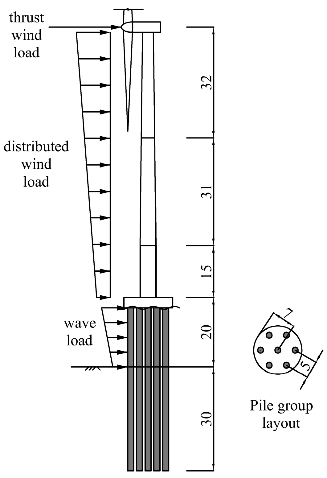
2.1. Model Establishment

As shown in Figure 2, the pile group supported 3.6 MW offshore wind turbine can be divided into two parts. The first part is the pile group foundation, which is partially embedded in the soil and partially submerged in the seawater. The second part is the superstructure, which is under distributed and thrust wind load.

2.2. Pile Submerged in the Seawater

The pile diameter of the pile group is relatively small compared with the wavelength ($D/L_{wl}\le 0.2$). Therefore, the wave load applied to the pile can be calculated by the Morison equation. For linear waves, at height z of the cylinder, the horizontal wave load $q_G(z)$ can be calculated according to Equation (1) [28]:

$$\begin{array}{c}{q}_G(z)=\frac{1}{2}{C}_D{\rho }_{w}D{\left(\frac{\pi H_w}{T}\frac{\cosh (K{Z}_w)}{\sinh (K{L}_w)}\right)}^2\cos \theta |\cos \theta |dz+\\ C_M\frac{\pi D^2}{4}\frac{2{\pi }^2{H}_w}{T^2}\frac{\cosh (K{Z}_w)}{\sinh (K{L}_w)}\sin \theta dz\end{array}$$

(1)

where $C_{\mathrm{D}}$ is the drag coefficient, $C_M$ is the inertia coefficient, $\theta =-\omega t$, ${\rho }_w$ is the density of the seawater, $D$ is the pile diameter, $H_w$ is the wave height, $T$ is the wave period, and $K=\frac{2\pi }{L_{wl}}$, where $L_{wl}$ is the wavelength. This paper mainly discusses the dynamic response of the pile under different frequencies; therefore, it is needed to calculate the maximum horizontal wave load applied to the whole pile body. The wave load applied to the whole pile body can be calculated according to Equation (2) [28]:

$$\begin{array}{l}{F}_T={\displaystyle {\int }_0^{L_w}{q}_G(z)=F_{HD}}\cos \theta |\cos \theta |+F_{HI}\sin \theta \\ F_{HD}=C_{\mathrm{D}}\frac{\gamma D{H}_w{}^2}{2}{K}_1,F_{HI}=C_M\frac{\gamma \pi D^2{H}_w}{8}{K}_2\end{array}$$

(2)

where $K_1=\frac{2K{L}_w+\sinh 2K{L}_w}{8\sinh 2K{L}_w}$ and $K_2=\tanh K{L}_w$. As shown in Equation (2), the value of $\theta$ to determine the maximum of $F_{HD}$ and $F_{HI}$ is not the same. Therefore, it is needed to determine the value of $\theta$ when the total wave force is the largest. According to the calculation, the maximum total wave force depends on the value of $F_{HD}$ and $F_{HI}$.

(1)

When $F_{HI}\ge 2F_{HD}$, the maximum total wave force happens when $\theta =\pi /2$, and the maximum total wave force $F_{T\max }$ equals $F_{HI}$.

(2)

When $F_{HI}<2F_{HD}$, the maximum total wave force happens when $\theta =\arcsin (F_{HI}/F_{HD})$, $F_{\max }=F_{HD}\left(1+\frac{1}{4}{\left(\frac{F_{HI}}{F_{HD}}\right)}^2\right)$.

In engineering, $F_{HI}<2F_{HD}$ is rarely seen. Therefore, in this paper, we consider $F_{HI}\ge 2F_{HD}$, which means $F_{T\max }=F_{HI}$. Then, we can calculate the wave load applied to the cylinder at height z when the maximum total wave load happens [28]:

$$q_G(z)=C_M\frac{\pi D^2}{4}\frac{2{\pi }^2{H}_w}{T^2}\frac{\cosh (K{Z}_w)}{\sinh (K{L}_w)}$$

(3)

Equation (3) is used for single piles in the seawater. However, the wave load applied to the pile group can be complex due to the pile–pile interaction and pile–cap interaction. According to the research [29], considering the pile–pile interaction, this paper considers the wave load applied to each pile within the pile group as 0.8 times the wave load applied to the single pile, and Equation (3) can be modified as:

$$q_G(z)=0.8C_M\frac{\pi D^2}{4}\frac{2{\pi }^2{H}_w}{T^2}\frac{\cosh (K{Z}_w)}{\sinh (K{L}_w)}$$

(4)

Based on the water–soil interface, the local coordinate system is established, and the $z$ axis is towards the seabed. The pile submerged in the seawater can be divided into n parts, and the length of each part is $h_i$. According to dynamic equilibrium conditions, the dynamic equation of each pile section can be obtained:

$$\frac{d^4{w}_i^{a1}}{d{z}^4}+4{\gamma }^4{w}_i^{a1}(z)=\frac{q_G(z)}{E_p{I}_p}$$

(5)

where $w$ is the lateral displacement of the pile section, superscript $a1$ denotes the first part of the active pile, and $\gamma ={(\frac{-m_p{\omega }^2}{4E_p{I}_p})}^{1/4}$, where $\omega$ is the load frequency, $m_p$ is the unit mass of the pile body, $E_p$ is the modulus of elasticity of the pile, and $I_p$ is the cross-section inertia moment of the pile. The solution of Equation (5) is the superposition of general solution and particular solution, as shown in Equation (6):

$$w_i^{a1}(z)=e^{(-1+i)\gamma z}{A}_{1i}^{a1}+e^{(-1-i)\gamma z}{A}_{2i}^{a1}+e^{(1-i)\gamma z}{A}_{3i}^{a1}+e^{(1+i)\gamma z}{A}_{4i}^{a1}+{q^{\prime }}_G(z)$$

(6)

where ${q^{\prime }}_G=a_p{q}_G,a_p=\frac{1}{E_p{I}_p(K^4+4{\gamma }^4)}$, $A_{1i}^{a1}$, $A_{2i}^{a1}$, $A_{3i}^{a1}$, $A_{4i}^{a1}$ are undetermined coefficients, which can be obtained according to boundary conditions.

According to differential relations, we can obtain the lateral displacement $w$, rotation angle $\theta$, bending moment $M$, and shearing force $Q$ of the pile section. For simplicity, we define $M=\overline{M}/E_p{I}_p$ and $Q=\overline{Q}/E_p{I}_p$ to represent the equivalent bending moment and shearing force. Written in matrix form:

$$\left\{\begin{array}{c}{w}_i^{a1}\\ {\varphi }_i^{a1}\\ M_i^{a1}\\ Q_i^{a1}\\ 1\end{array}\right\}=\left\{t_i^{a1}\right\}\left\{\begin{array}{c}{A}_{1i}^{a1}\\ A_{2i}^{a1}\\ A_{3i}^{a1}\\ A_{4i}^{a1}\\ 1\end{array}\right\}$$

(7)

where the matrix $\left\{t_i^{a1}\right\}$ is shown in Appendix A.

Equation (7) can be used to calculate each pile section of the pile body. The transfer matrix between the pile top and pile tip of each pile section can then be obtained, as shown in Equation (8):

$$\{\begin{array}{c}{w}^{a1}(h_i)\\ {\varphi }^{a1}(h_i)\\ M^{a1}(h_i)\\ Q^{a1}(h_i)\\ 1\end{array}\}=\left\{t_i^{a1}(h_i)\right\}{\left\{t_i^{a1}(0)\right\}}^{-1}\{\begin{array}{c}{w}^{a1}(0)\\ {\varphi }^{a1}(0)\\ M^{a1}(0)\\ Q^{a1}(0)\\ 1\end{array}\}$$

(8)

Let $\{T_i^{a1}\}=\left\{t_i^{a1}(h_i)\right\}{\left\{t_i^{a1}(0)\right\}}^{-1}$ and $T^{a1}=T_n^{a1}\cdots T_i^{a1}\cdots T_2^{a1}{T}_1^{a1}$; the transfer matrix between the pile tip (water–soil interface) and the pile top (water–air interface) can then be obtained, as shown in Equation (9):

$$\{\begin{array}{c}{w}^{a1}(L_w)\\ {\varphi }^{a1}(L_w)\\ M^{a1}(L_w)\\ Q^{a1}(L_w)\\ 1\end{array}\}=\{T^{a1}\}\{\begin{array}{c}{w}^{a1}(0)\\ {\varphi }^{a1}(0)\\ M^{a1}(0)\\ Q^{a1}(0)\\ 1\end{array}\}$$

(9)

Thus, we obtain the transfer matrix of the active pile submerged in the seawater. The solution can also be used for the passive pile and the active pile under the influence of the passive pile. Let $\{T^{p1}\}=\{T^{a1}\}=\{{\overline{T}}^{a1}\}$, written in matrix form:

$$\begin{array}{l}\{\begin{array}{c}{w}^{p1}(L_w)\\ {\varphi }^{p1}(L_w)\\ M^{p1}(L_w)\\ Q^{p1}(L_w)\\ 1\end{array}\}=\{T^{p1}\}\{\begin{array}{c}{w}^{p1}(0)\\ {\varphi }^{p1}(0)\\ M^{p1}(0)\\ Q^{p1}(0)\\ 1\end{array}\}\\ \{\begin{array}{c}{\overline{w}}^{a1}(L_w)\\ {\overline{\varphi }}^{a1}(L_w)\\ {\overline{M}}^{a1}(L_w)\\ {\overline{Q}}^{a1}(L_w)\\ 1\end{array}\}=\{{\overline{T}}^{a1}\}\{\begin{array}{c}{\overline{w}}^{a1}(0)\\ {\overline{\varphi }}^{a1}(0)\\ {\overline{M}}^{a1}(0)\\ {\overline{Q}}^{a1}(0)\\ 1\end{array}\}\end{array}$$

(10)

where $w^{p1}$ is the lateral displacement of the passive pile and ${\overline{w}}^{a1}$ is the lateral displacement of the active pile under the influence of the passive pile.

2.3. Pile Embedded in the Soil

2.3.1. Pile–Soil Interaction

The pile embedded in the soil is under lateral reaction of the soil. To investigate the influence of the soil cut-off frequency, this paper adopts the soil model proposed by Anoyatis [26]. This model uses the improved Tajimi soil model, considers the soil as a three-dimensional continuum, and considers the influence of soil vertical displacement on the lateral soil displacement. The proposed dynamic Winkler modulus can reflect the vibration of spring coefficient and damping coefficient around the soil cut-off frequency. The proposed calculation method is shown in the equation below:

$$\begin{array}{l}{k}^{\ast }=\pi G_s^{\ast }s\left[s+4\frac{Y_1{}^{\prime }(s)}{Y_0{}^{\prime }(s)}\right]\\ s=\frac{1}{2({\eta }_s)\chi }\sqrt{a_{cutoff}^2-\frac{a_0^2}{1+2i{\beta }_s}}\end{array}$$

(11)

where $G_s^{\ast }=G_s(1+2i{\beta }_s)$, ${\beta }_s$ is the soil material damping, valued 0.05 in this paper, ${Y^{\prime }}_1(s)$ and ${Y^{\prime }}_0(s)$ are the first and zero order modified Bessel function of the second kind, ${\eta }_s=\sqrt{2-{\nu }_s/1-{\nu }_s}$, where ${\upsilon }_s$ is Poisson’s ratio, $a_{\mathit{cutoff}}=(\pi /2){(L/D)}^{-1}$, where $L$ is the pile length, and $\chi$ is the dimensional coefficient, valued according to Poisson’s ratio, valued 3 in this paper.

As shown in Figure 3, the dynamic response of the pile embedded in the soil can be divided into four steps:

(1)

The horizonal displacement of the active pile under the pile top dynamic load;

(2)

The passive pile is influenced by the incident wave from the active pile displacement after the soil attenuation;

(3)

The horizontal displacement of the passive pile;

(4)

The active pile is influenced by the secondary wave from the passive pile displacement after soil attenuation.

2.3.2. Active Pile Displacement

The dynamic equation of the active pile under horizontal dynamic load can be written as:

$$\frac{d^4{w}_i^{a2}}{d{z}^4}+4{\gamma }^4{w}_i^{a2}(z)=0$$

(12)

where $\gamma ={(\frac{k+i\omega c-m_p{\omega }^2}{4E_p{I}_p})}^{1/4}$, $k=\mathrm{Re}(k^{*})$, $wc=\mathrm{IM}(k^{*})$, and $w_i^{a2}$ means the lateral displacement of the active pile embedded in the soil. The solution of Equation (12) is written below:

$$w_i^{a2}(z)=e^{(-1+i)\gamma z}{A}_{a2}+e^{(-1-i)\gamma z}{B}_{a2}+e^{(1-i)\gamma z}{C}_{a2}+e^{(1+i)\gamma z}{D}_{a2}$$

(13)

where $A_{a2}$, $B_{a2}$, $C_{a2}$, $D_{a2}$ are undetermined coefficients, which can be determined according to boundary conditions.

Similarly, according to differential relations, we can obtain the lateral displacement, rotation angle, bending moment, and shearing force of the active pile embedded in the soil. Written in matrix form:

$$\left\{\begin{array}{c}{w}_i^{a2}\\ {\varphi }_i^{a2}\\ M_i^{a2}\\ Q_i^{a2}\\ 1\end{array}\right\}=\left\{t_i^{a2}\right\}\left\{\begin{array}{c}{A}_{a2}\\ B_{a2}\\ C_{a2}\\ D_{a2}\\ 1\end{array}\right\}$$

(14)

where the matrix $\left\{t_i^{a2}\right\}$ is shown in Appendix A. The transfer matrix between the pile top and pile tip of each pile section is shown in Equation (15):

$$\{\begin{array}{c}{w}_i^{a2}(h_i)\\ {\varphi }_i^{a2}(h_i)\\ M_i^{a2}(h_i)\\ Q_i^{a2}(h_i)\\ 1\end{array}\}=\left\{t_i^{a2}(h_i)\right\}{\left\{t_i^{a2}(0)\right\}}^{-1}\{\begin{array}{c}{w}_i^{a2}(0)\\ w_i^{a2}(0)\\ M_i^{a2}(0)\\ Q_i^{a2}(0)\\ 1\end{array}\}$$

(15)

Let $\{T_i^{a2}\}=\left\{t_i^{a2}(h_i)\right\}{\left\{t_i^{a2}(0)\right\}}^{-1}$ and $T^{a2}=T_n^{a2}\cdots T_i^{a2}\cdots T_2^{a2}{T}_1^{a2}$; the transfer matrix between the active pile tip and top (soil-water surface) can be obtained:

$$\{\begin{array}{c}{w}^{a2}(H)\\ {\varphi }^{a2}(H)\\ M^{a2}(H)\\ Q^{a2}(H)\\ 1\end{array}\}=\{T^{a2}\}\{\begin{array}{c}{w}^{a2}(0)\\ {\varphi }^{a2}(0)\\ M^{a2}(0)\\ Q^{a2}(0)\\ 1\end{array}\}$$

(16)

2.3.3. Soil Attenuation Function and Soil Displacement

For the soil S m away from the active pile, its attenuation function and soil displacement can be calculated according to the following equation:

$$U_p(S,z)=\psi w^{a2}(z)=\left[\psi (S,0^{°})\cos {\theta }^2+\psi (S,{90}^{°})\sin {\theta }^2\right]w^{a2}(z)$$

(17)

where

$$\psi (S,0^{°})=\sqrt{\frac{R}{S}}\exp (\frac{-\beta \omega (R-S)}{V_{La}})\exp (\frac{-i\omega (R-S)}{V_{La}})$$

(18)

$$\psi (S,{90}^{°})=\sqrt{\frac{R}{S}}\exp (\frac{-\beta \omega (R-S)}{V_s})\exp (\frac{-i\omega (R-S)}{V_s})$$

(19)

where $R$ is the radius of the pile, $S$ is the distance between the active pile and passive pile, $\beta$ is the soil damping, $V_{La}$ and $V_s$ are the shear wave velocity and Lysmer’s simulation velocity [30], $V_{La}=\frac{3.4}{\pi (1-v)}{V}_s$, and $\theta$ is the angle of incidence, which will influence the pile–pile interaction factor, as shown in Figure 4.

The soil displacement around the passive pile after the soil attenuation can then be obtained. In pile groups, $\theta$ can be different between different piles, which will be considered when calculating the overall impedance of the pile group.

2.3.4. Passive Pile Displacement

The displacement of the passive pile due to the soil displacement can be calculated according to the following equation:

$$\frac{d^4{w}_i^{p2}}{d{z}^4}+4{\gamma }^4{w}_i^{p2}(z)-\frac{(k+i\omega c)}{E_p{I}_p}{U}_p(S,z)=0$$

(20)

Substitute Equation (17) into Equation (20), the solution can be obtained:

$$\begin{array}{ll}{w}_i^{p2}(z)=& e^{(-1+i)\gamma z}{A}_{p2}+e^{(-1-i)\gamma z}{B}_{p2}+e^{(1-i)\gamma z}{C}_{p2}+e^{(1+i)\gamma z}{D}_{p2}+\\ & \frac{(k+i\omega c)\psi z}{E_p{I}_p}[(1-i)e^{(-1+i)\gamma z}{A}_{a2}+(1+i)e^{(-1-i)\gamma z}{B}_{a2}+\\ & (-1+i)e^{(1-i)\gamma z}{C}_{a2}+(-1-i)e^{(1+i)\gamma z}{D}_{a2}]\end{array}$$

(21)

where $A_{p2}$, $B_{p2}$, $C_{p2}$, $D_{p2}$ are undetermined coefficients.

Written in matrix form:

$$\left\{\begin{array}{c}{w}_i^{p2}\\ {\varphi }_i^{p2}\\ M_i^{p2}\\ Q_i^{p2}\\ 1\end{array}\right\}=\left\{t_i^{a2}\right\}\left\{\begin{array}{c}{A}_{p2}\\ B_{p2}\\ C_{p2}\\ D_{p2}\\ 1\end{array}\right\}+\left\{t_i^{p2}\right\}\left\{\begin{array}{c}{A}_{a2}\\ B_{a2}\\ C_{a2}\\ D_{a2}\\ 1\end{array}\right\}$$

(22)

where the matrix $\left\{t_i^{p2}\right\}$ is shown in Appendix A. The transfer matrix between passive pile segment tip and top can be obtained after the following calculation:

$$\left\{\begin{array}{c}{w}_i^{p2}(h_i)\\ {\varphi }_i^{p2}(h_i)\\ M_i^{p2}(h_i)\\ Q_i^{p2}(h_i)\\ 1\end{array}\right\}=T_{i1}^{p2}\left\{\begin{array}{c}{w}_i^{p2}(0)\\ {\varphi }_i^{p2}(0)\\ M_i^{p2}(0)\\ Q_i^{p2}(0)\\ 1\end{array}\right\}+T_{i2}^{p2}\{\begin{array}{c}{w}_i^{a2}(0)\\ w_i^{a2}(0)\\ M_i^{a2}(0)\\ Q_i^{a2}(0)\\ 1\end{array}\}$$

(23)

where

$$\begin{array}{l}{T}_{i1}^{p2}=t_i^{a2}(h_i){\left(t_i^{a2}(0)\right)}^{-1}\\ T_{i2}^{p2}=\left(t_i^{p2}(h_i)-t_i^{a2}(h_i){\left(t_i^{a2}(0)\right)}^{-1}{t}_i^{p2}(0)\right){\left(t_i^{a2}(0)\right)}^{-1}\end{array}$$

(24)

The transfer matrix between the passive pile tip and top (soil-water surface) can then be obtained:

$$\left\{\begin{array}{c}{w}_{}^{p2}(H)\\ {\varphi }_{}^{p2}(H)\\ M_{}^{p2}(H)\\ Q_{}^{p2}(H)\\ 1\end{array}\right\}=T_1^{p2}\left\{\begin{array}{c}{w}_{}^{p2}(0)\\ {\varphi }_{}^{p2}(0)\\ M_{}^{p2}(0)\\ Q_{}^{p2}(0)\\ 1\end{array}\right\}+T_2^{p2}\{\begin{array}{c}{w}_{}^{a2}(0)\\ w_{}^{a2}(0)\\ M_{}^{a2}(0)\\ Q_{}^{a2}(0)\\ 1\end{array}\}$$

(25)

where $T_1^{p2}=T_{n1}^{p2}\cdots T_{i1}^{p2}\cdots T_{21}^{p2}{T}_{11}^{p2}$, $T_2^{p2}=T_{n2}^{p2}\cdots T_{i2}^{p2}\cdots T_{22}^{p2}{T}_{12}^{p2}$.

2.3.5. Active Pile Displacement Due to Secondary Wave

The passive pile displacement will produce secondary wave, which will influence the active pile displacement. The soil displacement around the active pile can be calculated according to the following equation:

$$U_a(S,z)=\psi w^{p2}(z)=\left[\psi (S,0^{°})\cos {\theta }^2+\psi (S,{90}^{°})\sin {\theta }^2\right]w^{p2}(z)$$

(26)

The dynamic equation can be written as:

$$\frac{d^4{\overline{w}}_i^{a2}}{d{z}^4}+4{\gamma }^4{\overline{w}}_i^{a2}(z)-\frac{(k+i\omega c)}{E_p{I}_p}{U}_a(S,z)=0$$

(27)

where ${\overline{w}}^{a2}$ is the lateral displacement of the active pile under the influence of the passive pile. The solution to Equation (27) is:

$$\begin{array}{ll}{\overline{w}}_i^{a2}(z)=& e^{(-1+i)\gamma z}{\overline{A}}_{a2}+e^{(-1-i)\gamma z}{\overline{B}}_{a2}+e^{(1-i)\gamma z}{\overline{C}}_{a2}+e^{(1+i)\gamma z}{\overline{D}}_{a2}+\\ & \frac{(k+i\omega c)\psi z}{16E_p{I}_p{\gamma }^3}[(1-i)e^{(-1+i)\gamma z}{A}_{p2}+(1+i)e^{(-1-i)\gamma z}{B}_{p2}+\\ & (-1+i)e^{(1-i)\gamma z}{C}_{p2}+(-1-i)e^{(1+i)\gamma z}{D}_{p2}]+\\ & \frac{(k+i\omega c)\psi z^2}{512E_p{I}_p{\gamma }^6}[{(1-i)}^2{e}^{(-1+i)\gamma z}{A}_{a2}+{(1+i)}^2{e}^{(-1-i)\gamma z}{B}_{a2}+\\ & {(-1+i)}^2{e}^{(1-i)\gamma z}{C}_{a2}+{(-1-i)}^2{e}^{(1+i)\gamma z}{D}_{a2}]\end{array}$$

(28)

where ${\overline{A}}_{a2}$, ${\overline{B}}_{a2}$, ${\overline{C}}_{a2}$, ${\overline{D}}_{a2}$ are undetermined coefficients.

Written in matrix form:

$$\begin{array}{l}\left\{\begin{array}{c}{\overline{w}}_i^{a2}\\ {\overline{\varphi }}_i^{a2}\\ {\overline{M}}_i^{a2}\\ {\overline{Q}}_i^{a2}\\ 1\end{array}\right\}=\left\{t_i^{a2}\right\}\left\{\begin{array}{c}{\overline{A}}_{a2}\\ {\overline{B}}_{a2}\\ {\overline{C}}_{a2}\\ {\overline{D}}_{a2}\\ 1\end{array}\right\}+\frac{1}{16{\gamma }^3}\left\{t_i^{p2}\right\}\left\{\begin{array}{c}{A}_{p2}\\ B_{p2}\\ C_{p2}\\ D_{p2}\\ 1\end{array}\right\}+\\ \left(\left\{{\overline{t}}_i^{a2}\right\}+\frac{3i}{1024{\gamma }^7}\left\{\begin{array}{cccc}{(1-i)}^2& 0& 0& 0\\ 0& {(1+i)}^2& 0& 0\\ 0& 0& {(-1+i)}^2& 0\\ 0& 0& 0& {(-1-i)}^2\end{array}\right\}\left\{t_i^{p2}\right\}\right)\left\{\begin{array}{c}{A}_{a2}\\ B_{a2}\\ C_{a2}\\ D_{a2}\\ 1\end{array}\right\}\end{array}$$

(29)

where the matrix $\left\{{\overline{t}}_i^{a2}\right\}$ is shown in Appendix A.

Let:

$$\begin{array}{l}\left\{t_i^1\right\}=\left\{t_i^{a2}\right\}\\ \left\{t_i^2\right\}=\frac{1}{16{\gamma }^3}\left\{t_i^{p2}\right\}\\ \left\{t_i^3\right\}=\left\{{\overline{t}}_i^{a2}\right\}+\frac{3i}{1024{\gamma }^7}\left\{\begin{array}{cccc}{(1-i)}^2& 0& 0& 0\\ 0& {(1+i)}^2& 0& 0\\ 0& 0& {(-1+i)}^2& 0\\ 0& 0& 0& {(-1-i)}^2\end{array}\right\}\left\{t_i^{p2}\right\}\end{array}$$

(30)

Equation (29) can be simplified:

$$\left\{\begin{array}{c}{\overline{w}}_i^{a2}\\ {\overline{\varphi }}_i^{a2}\\ {\overline{M}}_i^{a2}\\ {\overline{Q}}_i^{a2}\\ 1\end{array}\right\}=\left\{t_i^1\right\}\left\{\begin{array}{c}{\overline{A}}_{a2}\\ {\overline{B}}_{a2}\\ {\overline{C}}_{a2}\\ {\overline{D}}_{a2}\\ 1\end{array}\right\}+\left\{t_i^2\right\}\left\{\begin{array}{c}{A}_{p2}\\ B_{p2}\\ C_{p2}\\ D_{p2}\\ 1\end{array}\right\}+\left\{t_i^3\right\}\left\{\begin{array}{c}{A}_{a2}\\ B_{a2}\\ C_{a2}\\ D_{a2}\\ 1\end{array}\right\}$$

(31)

The transfer matrix between active pile segment tip and top can then be obtained:

$$\left\{\begin{array}{c}{\overline{w}}_i^{a2}(h_i)\\ {\overline{\varphi }}_i^{a2}(h_i)\\ {\overline{M}}_i^{a2}(h_i)\\ {\overline{Q}}_i^{a2}(h_i)\\ 1\end{array}\right\}=T_{i1}\left\{\begin{array}{c}{\overline{w}}_i^{a2}(0)\\ {\overline{\varphi }}_i^{a2}(0)\\ {\overline{M}}_i^{a2}(0)\\ {\overline{Q}}_i^{a2}(0)\\ 1\end{array}\right\}+T_{i2}\{\begin{array}{c}{w}_i^{p2}(0)\\ w_i^{p2}(0)\\ M_i^{p2}(0)\\ Q_i^{p2}(0)\\ 1\end{array}\}+T_{i3}\{\begin{array}{c}{w}_i^{a2}(0)\\ w_i^{a2}(0)\\ M_i^{a2}(0)\\ Q_i^{a2}(0)\\ 1\end{array}\}$$

(32)

where

$$\begin{array}{ll}{T}_{i1}=& t_i^1(h_i){\left(t_i^1(0)\right)}^{-1}\\ T_{i2}=& \left(t_i^2(h_i)-t_i^1(h_i){\left(t_i^1(0)\right)}^{-1}{t}_i^2(0)\right){\left(t_i^{a2}(0)\right)}^{-1}\\ T_{i3}=& -\left(t_i^2(h_i)-t_i^1(h_i){\left(t_i^1(0)\right)}^{-1}{t}_i^2(0)\right){\left(t_i^{a2}(0)\right)}^{-1}{t}_i^{p2}(0){\left(t_i^{a2}(0)\right)}^{-1}+\\ & \left(t_i^3(h)-t_i^1(h){\left(t_i^1(0)\right)}^{-1}{t}_i^3(0)\right){\left(t_i^{a2}(0)\right)}^{-1}\end{array}$$

(33)

The transfer matrix between the active pile tip and top (soil–water surface) due to the secondary wave can then be obtained:

$$\left\{\begin{array}{c}{\overline{w}}_{}^{a2}(H)\\ {\overline{\varphi }}_{}^{a2}(H)\\ {\overline{M}}_{}^{a2}(H)\\ {\overline{Q}}_{}^{a2}(H)\\ 1\end{array}\right\}=T_1\left\{\begin{array}{c}{\overline{w}}_{}^{a2}(0)\\ {\overline{\varphi }}_{}^{a2}(0)\\ {\overline{M}}_{}^{a2}(0)\\ {\overline{Q}}_{}^{a2}(0)\\ 1\end{array}\right\}+T_2\{\begin{array}{c}{w}_{}^{p2}(0)\\ w_{}^{p2}(0)\\ M_{}^{p2}(0)\\ Q_{}^{p2}(0)\\ 1\end{array}\}+T_3\{\begin{array}{c}{w}_{}^{a2}(0)\\ w_{}^{a2}(0)\\ M_{}^{a2}(0)\\ Q_{}^{a2}(0)\\ 1\end{array}\}$$

(34)

where $T_1=T_{n1}\cdots T_{i1}\cdots T_{21}{T}_{11}$, $T_2=T_{n2}\cdots T_{i2}\cdots T_{22}{T}_{12}$, $T_3=T_{n3}\cdots T_{i3}\cdots T_{23}{T}_{13}$.

2.4. Overall Dynamic Response of the Pile Group

The transfer matrix of pile submerged in the seawater and pile embedded in the soil are obtained in Section 2.3 and Section 2.4. According to the continuity condition at the water–soil interface, the dynamic response of these two pile parts can be connected, and the overall dynamic response of the pile can be obtained.

2.4.1. Active Pile

For the active pile, the continuity condition is:

$$\{\begin{array}{c}{w}^{a2}(0)\\ {\varphi }^{a2}(0)\\ M^{a2}(0)\\ Q^{a2}(0)\\ 1\end{array}\}=\{\begin{array}{c}{w}^{a1}(L_w)\\ {\varphi }^{a1}(L_w)\\ M^{a1}(L_w)\\ Q^{a1}(L_w)\\ 1\end{array}\}$$

(35)

Substituting Equations (10) and (35) into Equation (16), the overall transfer matrix can be obtained:

$$\{\begin{array}{c}{w}^a(L)\\ {\varphi }^a(L)\\ M^a(L)\\ Q^a(L)\\ 1\end{array}\}=\{T^{a2}\}\{T^{a1}\}\{\begin{array}{c}{w}^a(0)\\ {\varphi }^a(0)\\ M^a(0)\\ Q^a(0)\\ 1\end{array}\}$$

(36)

Substituting boundary conditions:

$$\begin{array}{l}{M_{z=0}=\frac{d^{2}w(z)}{d{z}^2}|}_{z=0}=0\\ {Q_{z=0}=\frac{d^{3}w(z)}{d{z}^3}|}_{z=0}=0\\ {w_{z=L}=w(z)|}_{z=L}=0\\ {{\theta }_{z=L}=\frac{dw(z)}{dz}|}_{z=L}=0\end{array}$$

(37)

Equation (36) can then be solved, and the displacement, rotation angle, bending moment and the shearing force of the active pile top can be obtained; the value of single pile swaying impedance $K_{hh}^{*}$, rocking impedance $K_{rr}^{*}$, swaying-rocking impedance $K_{hr}^{*}$, and rocking-swaying impedance $K_{rh}^{*}$ can then be obtained.

2.4.2. Passive Pile

For the passive pile, the continuity condition is:

$$\{\begin{array}{c}{w}^{p2}(0)\\ {\varphi }^{p2}(0)\\ M^{p2}(0)\\ Q^{p2}(0)\\ 1\end{array}\}=\{\begin{array}{c}{w}^{p1}(L_w)\\ {\varphi }^{p1}(L_w)\\ M^{p1}(L_w)\\ Q^{p1}(L_w)\\ 1\end{array}\}$$

(38)

Substituting Equations (10), (11) and (38) into Equation (25), the overall transfer matrix can be obtained:

$$\left\{\begin{array}{c}{w}_{}^p(L)\\ {\varphi }_{}^p(L)\\ M_{}^p(L)\\ Q_{}^p(L)\\ 1\end{array}\right\}=\left\{T_1^{p2}\right\}\left\{T^{p1}\right\}\{\begin{array}{c}{w}^p(0)\\ {\varphi }^p(0)\\ M^p(0)\\ Q^p(0)\\ 1\end{array}\}+\left\{T_2^{p2}\right\}\left\{T^{a1}\right\}\{\begin{array}{c}{w}^a(0)\\ {\varphi }^a(0)\\ M^a(0)\\ Q^a(0)\\ 1\end{array}\}$$

(39)

Substituting the solution to Equation (36) and boundary conditions (37), the equation can then be solved, and the displacement, rotation angle, bending moment, and the shearing force of the passive pile top can be obtained.

2.4.3. Active Pile under Secondary Wave

For the active pile under secondary wave:

$$\{\begin{array}{c}{\overline{w}}^{a2}(0)\\ {\overline{\varphi }}^{a2}(0)\\ {\overline{M}}^{a2}(0)\\ {\overline{Q}}^{a2}(0)\\ 1\end{array}\}=\{\begin{array}{c}{\overline{w}}^{a1}(L_w)\\ {\overline{\varphi }}^{a1}(L_w)\\ {\overline{M}}^{a1}(L_w)\\ {\overline{Q}}^{a1}(L_w)\\ 1\end{array}\}$$

(40)

Substituting Equations (10), (11) and (40) into Equation (34), the overall transfer matrix can be obtained:

$$\left\{\begin{array}{c}{\overline{w}}_{}^a(L)\\ {\overline{\varphi }}_{}^a(L)\\ {\overline{M}}_{}^a(L)\\ {\overline{Q}}_{}^a(L)\\ 1\end{array}\right\}=T_1\{{\overline{T}}^{a1}\}\left\{\begin{array}{c}{\overline{w}}_{}^a(0)\\ {\overline{\varphi }}_{}^a(0)\\ {\overline{M}}_{}^a(0)\\ {\overline{Q}}_{}^a(0)\\ 1\end{array}\right\}+T_2\{T^{p1}\}\{\begin{array}{c}{w}^p(0)\\ {\varphi }^p(0)\\ M^p(0)\\ Q^p(0)\\ 1\end{array}\}+T_3\{T^{a1}\}\{\begin{array}{c}{w}^a(0)\\ {\varphi }^a(0)\\ M^a(0)\\ Q^a(0)\\ 1\end{array}\}$$

(41)

Substituting the solutions to Equations (36) and (39), and boundary conditions (37), the equation can be solved. The displacement, rotation angle, bending moment, and the shearing force of the active pile top under the secondary wave can be obtained.

2.4.4. Pile–Pile Interaction and Pile Group Dynamic Response

The pile–pile interaction factor is defined as [31]:

$${\alpha }^G=\frac{w^p}{w^a}$$

(42)

where $w_a$ is the displacement of the active pile and $w_p$ is the displacement of the passive pile. To reflect the influence of the passive pile to the active pile, the definition of the pile–pile interaction factor is modified as [32]:

$$\begin{array}{l}{\alpha }^G=\frac{w^p}{w^a-{\overline{w}}^a}=\frac{w^p}{(1-\kappa )w^a}\\ \kappa =\frac{{\overline{w}}^a}{w^a}\end{array}$$

(43)

where ${\overline{w}}_a$ is the displacement of active pile under secondary wave.

Suppose the number of piles of the pile group is n, the cap is rigid, and the mass of the cap is ignored. Under the lateral harmonic load $P{e}^{i\omega t}$, the lateral displacement of the pile group $w^G$ can be considered equal to the displacement of each pile $w^i$, which means $w^1=w^i=w^G$. In the pile group, each pile plays the role of both active pile and passive pile, so the single pile displacement can be calculated:

$$w^i=(1-{\displaystyle \sum _{j=1,j\ne i}^n{\kappa }_{ij}})w^i+{\displaystyle \sum _{j=1,j\ne i}^n{\alpha }_{ij}^G}{w}^j$$

(44)

The dynamic equation of the pile group can be written in matrix form:

$$\frac{1}{K_{hh}^{*}}[\begin{array}{cccc}1-{\displaystyle \sum _{j=1,j\ne 1}^n{\kappa }_{1j}}& {\alpha }_{12}^G& \cdots & {\alpha }_{1n}^G\\ {\alpha }_{21}^G& 1-{\displaystyle \sum _{j=1,j\ne 2}^n{\kappa }_{2j}}& \cdots & {\alpha }_{2n}^G\\ ⋮& ⋮& ⋮& ⋮\\ {\alpha }_{n1}^G& {\alpha }_{n2}^G& \cdots & 1-{\displaystyle \sum _{j=1,j\ne n}^n{\kappa }_{nj}}\end{array}]\{\begin{array}{c}{P}_1\\ P_2\\ ⋮\\ P_n\end{array}\}=\{\begin{array}{c}{w}^1\\ w^2\\ ⋮\\ w^n\end{array}\}$$

(45)

where $K_{hh}^{*}$ is the single pile impedance, which can be obtained by solving the Equation (36), $P_j$ is the load distributed to pile $j$, and $a_{ij}^G$ is the interaction factor between pile $i$ and $j$, $i\ne j$. The load applied to the pile group is the sum of the load applied to each pile:

$$P={\displaystyle \sum _{j=1}^n{P}_j}$$

(46)

Then, Equation (45) can be solved, and the horizontal pile group impedance can be calculated:

$$K_G^{*}=P/w_G=K_G+i{C}_G$$

(47)

According to the previous research [31], the swaying interaction factor, the sway-rocking interaction factor, and the rock-swaying interaction factor between piles can be ignored. Therefore, $K_{rr}^{*}$, $K_{hr}^{*}$ $K_{rh}^{*}$ are the sum of single pile calculation results. The pile group impedance matrix can then be obtained:

$$K^{*}=\{\begin{array}{cc}{K}_G^{*}& K_{hr}^{*}\\ K_{rh}^{*}& K_{rr}^{*}\end{array}\}$$

(48)

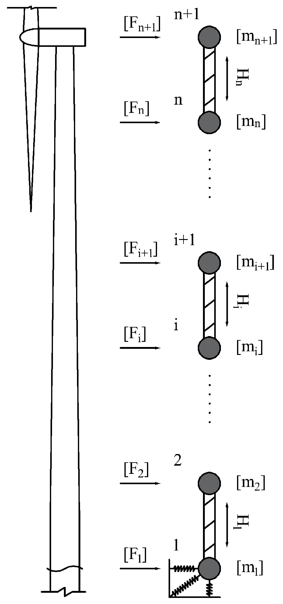
2.5. Superstructure Dynamic Response

2.5.1. Distributed Wind Load

The distributed wind load $F_d(z)$ can be calculated according to the equation below [33]:

$$F_d(z)=1/2{\rho }_a{C}_D{D}_T(z)V^2(z)$$

(49)

where ${\rho }_d$ is the density of the air, valued 1.225 kg/m³ in this paper, $C_{\mathrm{D}}$ is the drag coefficient, valued according to the Reynolds number and structure surface roughness, i.e., 1.2 in this paper, $V$ (m/s) is the average wind speed, and $D_T$ (m) is the tower diameter, the value of which changes with increasing tower height.

The wind profile [34] can be calculated according to the following equation:

$$V(z)=V_a{(\frac{z}{H_a})}^{{\alpha }_w}$$

(50)

where $V_a$ is the wind speed at height $H_a$ and ${\alpha }_w$ is the power law coefficient, valued 0.12 in open seas with waves.

2.5.2. Thrust Wind Load

The wind load applied to the blades and turbine will produce lateral load, which can be considered as the concentrated load $F_b$, calculated according to Equation (51) [35]:

$$F_b=1/2{\rho }_a\pi R_T^2{V}_T^2{C}_T({\lambda }_s)$$

(51)

where $V_T$ is the wind speed at the tower top, $R_T$ is the blade radius, and $C_T$ is the thrust coefficient, which is related to the tip speed ratio ${\lambda }_s$, as shown in Figure 5.

2.5.3. Tower Dynamic Response

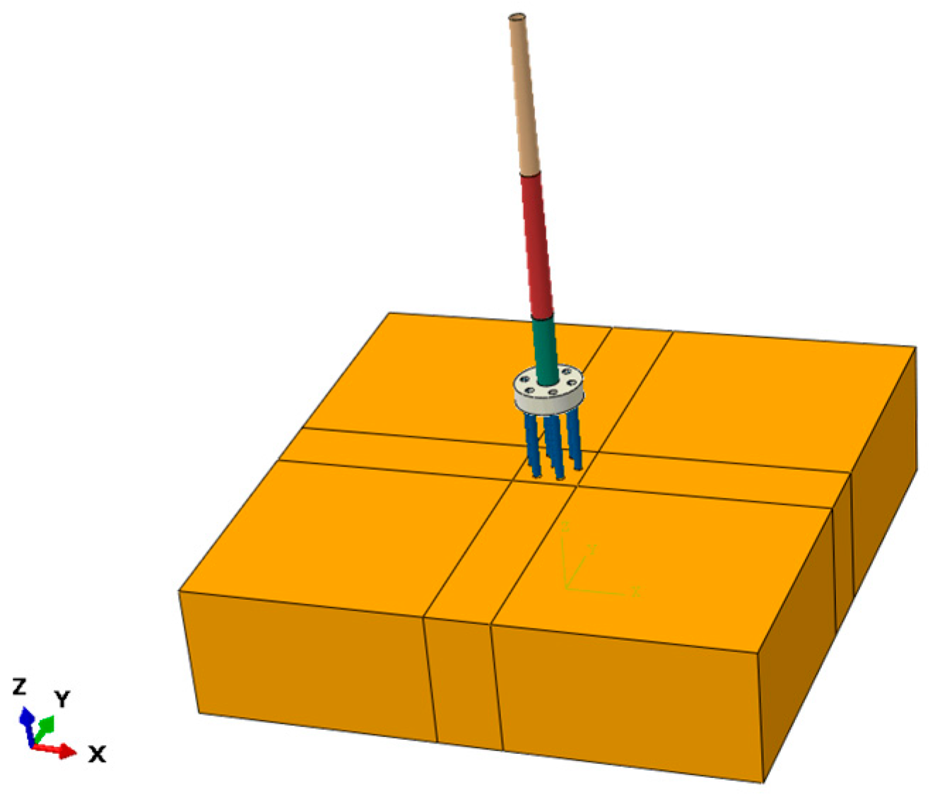
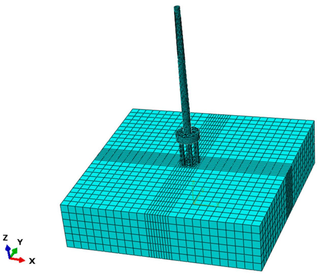
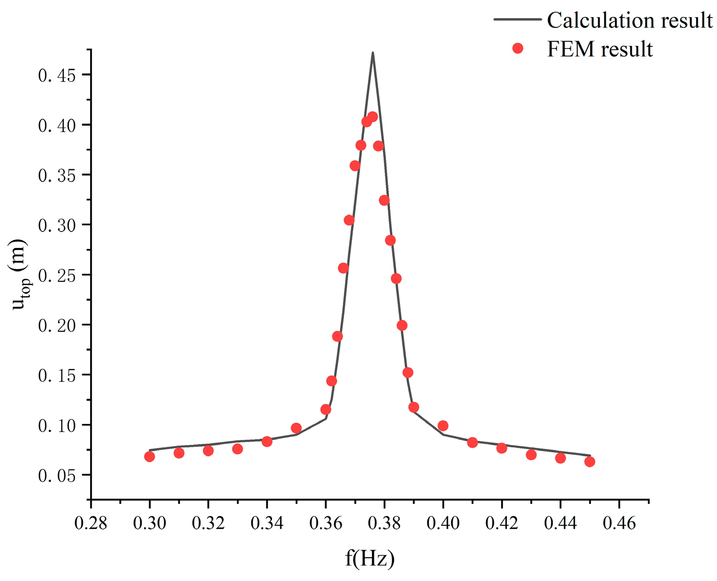
The tower can be divided into n segments, numbered 1~$n$ from the bottom to the top. As shown in Figure 6, for the $i$ ($i=1,2\cdots n$)th segment, the number of its bottom point is $i$, and the number of its top point is $i+1$. Consider each segment as equal cross-section beam, where $H_i$ is the length of the $i$th segment. $H_i$ is valued differently between segments to account for the varied cross-section geometry. The mass of each segment is concentrated to the bottom point, and the $2\times 2$ mass matrix of each segment can be obtained, including the mass and moment of inertia. The mass of blades is considered as the concentrated mass point $m_{n+1}$ at the tower top. Similarly, the distributed loads applied to each segment are concentrated to the bottom point, and the load matrix of each segment can be obtained, including the force and bending moment. The load matrix at the tower top includes the thrust wind force.

The swaying-rocking equation of this system with 2($n$+1) degrees of freedom can be written in matrix form [25]:

$$\left[\begin{array}{ccccccc}{\overline{K}}_{11}& {\overline{K}}_{12}& & & & & \\ {\overline{K}}_{21}& {\overline{K}}_{22}& {\overline{K}}_{23}& & & & \\ & \ddots & \ddots & \ddots & & & \\ & & {\overline{K}}_{i,j-1}& {\overline{K}}_{i,j}& {\overline{K}}_{i,j+1}& & \\ & & & \ddots & \ddots & \ddots & \\ & & & & {\overline{K}}_{n,n-1}& {\overline{K}}_{n,n}& {\overline{K}}_{n,n+1}\\ & & & & & {\overline{K}}_{n+1,n}& {\overline{K}}_{n+1,n+1}\end{array}\right]\left\{\begin{array}{c}{u}_1\\ u_2\\ ⋮\\ u_i\\ ⋮\\ u_n\\ u_{n+1}\end{array}\right\}=\left\{\begin{array}{c}{F}_1\\ F_2\\ ⋮\\ F_i\\ ⋮\\ F_n\\ F_{n+1}\end{array}\right\}$$

(52)

where $u_i$ is the point displacement matrix, including the horizontal displacement and rotation angle. The stiffness in Equation (52) can be calculated according to equations below.

For the first line:

$${\overline{K}}_{11}=K_{11}+K^{*}-{\omega }^2{m}_1$$

(53)

$${\overline{K}}_{12}=K_{12}$$

(54)

For the second to $n$th line:

$${\overline{K}}_{i,i-1}=K_{i,i-1}$$

(55)

$${\overline{K}}_{i,i}=K_{i,i}-{\omega }^2{m}_i$$

(56)

$${\overline{K}}_{i,i+1}=K_{i,i+1}$$

(57)

For $n+1$th line:

$${\overline{K}}_{n+1,n}=K_{n+1,n}$$

(58)

$${\overline{K}}_{n+1,n+1}=K_{n+1,n+1}-{\omega }^2{m}_{n+1}$$

(59)

where

$$K_{i,i-1}=\left[\begin{array}{cc}-12E_p{I}_{i-1}/H_{i-1}^3& -6E_p{I}_{i-1}/H_{i-1}^2\\ 6E_p{I}_{i-1}/H_{i-1}^2& 2E_p{I}_{i-1}/H_{i-1}\end{array}\right]$$

(60)

$$K_{i,i}=\left[\begin{array}{cc}12E_p{I}_i/H_i^3& 6E_p{I}_i/H_i^2\\ 6E_p{I}_i/H_i^2& 4E_p{I}_i/H_i\end{array}\right]+\left[\begin{array}{cc}12E_p{I}_{i-1}/H_{i-1}^3& -6E_p{I}_{i-1}/H_{i-1}^2\\ -6E_p{I}_{i-1}/H_{i-1}^2& 4E_p{I}_{i-1}/H_{i-1}\end{array}\right]$$

(61)

$$K_{i,j+1}=\left[\begin{array}{cc}-12E_p{I}_i/H_i^3& 6E_p{I}_i/H_i^2\\ -6E_p{I}_i/H_i^2& 2E_p{I}_i/H_i\end{array}\right]$$

(62)

When $i=1$, Equation (60) is invalid, and the second part of Equation (61) should be removed. When $i=n+1$, Equation (57) is invalid, and the first part of Equation (61) should be removed. Substitute the foundation impedance matrix $K^{*}$ into Equation (53), the equation can then be solved, and the displacement of the tower can be obtained.

3. Validation

The calculation result is compared with the FEM result to validate the correctness of the proposed calculation model. ABAQUS simulation software is used in this paper. A pile group supported OWT [25] is used for validation. The total mass of blades and turbine is 177.1 ton, and the tower is divided into three segments, as shown in

Table 1. Tower parameters.

Tower Parts	Length (m)	Bottom Diameter	Top Diameter	Tower Wall Thickness
Upper segment	32	3.9	3.1	50
Middle segment	31	4.5	3.9	50
Bottom segment	15	4.5	4.5	50

. The pile group consists of seven piles, as shown in Figure 2. The pile diameter is 1.7 m and the pile wall thickness is 30 mm. The elastic modulus of the steel is 210 GPa and the density of the steel is 7800 kg/m³. The pile length embedded in the soil is 30 m nad the pile length submerged in the seawater is 20 m. The elastic modulus of the soil is 40 MPa, the Poisson’s ratio of the soil is 0.3, and the density of the soil is 1800 kg/m³. As shown in Figure 7, the offshore wind turbine model is established.

Since the overall displacement of the offshore wind turbine is relatively small, linear modal analysis is used to calculate its structure natural frequency. The deformation of soil foundation is also small during the dynamic analysis; therefore, the change of soil foundation stiffness is not considered, and the small strain linear elastic model is used for the soil.

For the tower, the eight-node S8R shell element is used. The tower is divided into three parts, as shown in Table 1. For each part, the tower diameter changes linearly with increasing height. To prevent the separation between tower parts, a bonding constraint is added between the interfaces, including the interface between the bottom tower part and the cap. The blades are simplified as the concentrated force applied to the tower top. The pile foundation is modeled as solid element to better simulate the pile–soil interaction. For the side face of the soil, the lateral displacement is constrained; for the bottom side of the soil, displacements of all directions are constrained. The pile–soil interaction is set as small sliding, penalty contact, while the coefficient is set as 0.4.

The dead weight is applied to the model according to parameters presented in Table 1, and the wave load is also applied to the structure. Here, we use FORTRAN to write a subroutine to accurately input wave load according to Equation (4). The offshore wind turbine is fine meshed. As for the soil, the soil around the pile is refined, as shown in Figure 8.

After establishing the FEM model, the modal analysis is performed, and the first 10 structure natural frequencies are obtained. Here, we focus on the first lateral structure natural frequency. Then, we applied a 10 kN horizontal harmonic thrust wind load to the tower top, and the tower top displacement and load frequency curve can be obtained.

As shown in Figure 9, the FEM result and the calculating result are in good agreement, with only some differences being observed for the maximum tower displacement, which validates the correctness of the calculating result. The structure natural frequency can also be obtained from Figure 9, which falls within the “soft-stiff” design frequency range.

4. Parametric Analysis

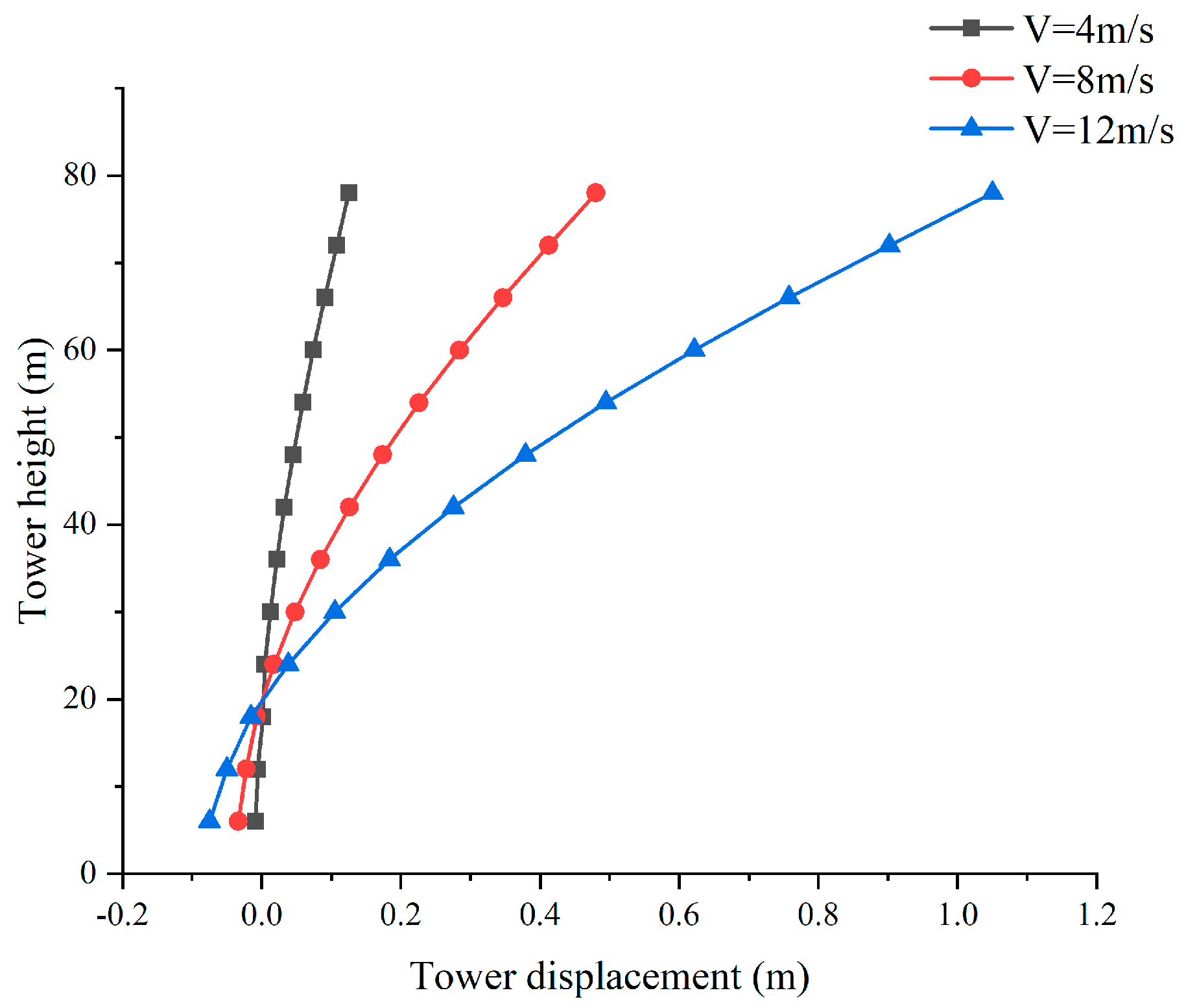
4.1. Tower Displacement

The tower displacement under different wind speeds is studied. The wind speed at sea level is 4 m/s, 8 m/s, and 12 m/s, respectively. The percentage of the thrust wind load is 96.31%, and the percentage of the distributed wind load is 3.69%. As shown in Figure 10, the tower displacement is largely influenced by the wind speed. When the wind speed is 4 m/s, the increasing rate of tower displacement is relatively small. When the wind speed is 8 m/s, the increasing rate rises to a certain degree. When the wind speed is 12 m/s, the increasing rate is significantly larger than the increasing rate when the wind speed is 4 m/s.

The influence of the foundation impedance on the tower displacement is also studied. Define ${\alpha }_K={K^{\prime }}^{*}/K^{*}$, where ${K^{\prime }}^{*}$ is the modified foundation impedance matrix and ${\alpha }_K$ is valued from 0.1~2 to analyze the influence of the foundation impedance on the maximum tower displacement. As shown in Figure 11, when the foundation impedance is relatively small, the tower displacement is large. With increasing foundation impedance, the tower displacement decreases rapidly. Additionally, with increasing foundation impedance, the tower displacement decreasing speed slows. When the foundation impedance reaches 2.0 its original impedance, the tower displacement remains almost unchanged.

4.2. Pile–Pile Interaction Factor

The regressive solution (the pile is considered completely embedded in the soil) of the proposed calculation model is compared with the solution of Kaynia [36]. In this section, parameters below are used for calculation: the ratio of elastic modulus of the pile to elastic modulus of the soil $E_p/E_s=1000$, the ratio of the pile length to the pile diameter $L/D=20$, and Poisson’s ratio is 0.4. The ratio of the density of the pile to the density of the soil ${\rho }_p/{\rho }_s=1.3$, while the damping ratio ${\beta }_s=0.05$. The pile spacing $S=2D$, the pile embedment ratio $L_w/L=0.3$. The dimensionless frequency $a_0=\omega D/V_s$ is used for analysis. Here, we consider the influence of three parameters on the pile–pile interaction factor: pile spacing, pile embedment ratio, and the angle of incidence $\theta$.

As shown in Figure 12, when the pile spacing $S/D=10$, the calculating result of this paper and the result from the literature are in good agreement, which validates the correctness of the calculation method. When the pile spacing $S/D=5$, some differences can be observed compared with the results from the literature. Furthermore, when $S/D=2$, the difference becomes more significant, especially in low frequencies. This is because when the pile spacing decreases, the influence of the passive pile on the active pile is more significant, which changes the horizontal displacement of the active pile. This analysis demonstrates that when the pile spacing is small, the influence of the passive pile on the active pile is important and cannot be ignored.

The influence of the pile embedded ratio is studied. As shown in Figure 13, when the pile is completely embedded, the pile–pile interaction factor decreases with increasing load frequency, and the value remains positive. When $L_w/L=0.1$, the pile–pile interaction factor $\alpha$ at all frequencies largely decreases. When $L_w/L=0.2$, $\alpha$ changes obviously. With increasing load frequency, $\alpha$ decreases rapidly when closing to a certain frequency and rises after reaching the lowest point. When $L_w/L=0.3$, the curve moves from a mainly middle-high frequency to a middle-low frequency. This analysis demonstrates that $\alpha$ is sensitive to the pile embedment ratio. When the pile embedment ratio is relatively small, the change of $\alpha$ with increasing frequency is simple; when the pile embedment ratio is relatively large, the change of $\alpha$ becomes complex.

The influence of different incidences angle $\theta$ is studied, i.e., $0^{°}$, ${45}^{°}$, and ${90}^{°}$, respectively. As shown in Figure 14, when $\theta =0^{°}$, the curve fluctuates significantly, the minimum value of $\alpha$ is the smallest among three angles, and the maximum value of $\alpha$ is the largest among three angles. When $\theta ={90}^{°}$, the value of $\alpha$ is slightly smaller than that of $\theta =0^{°}$. When $\theta ={45}^{°}$, the change of $\alpha$ is moderate, and no significant fluctuation is observed.

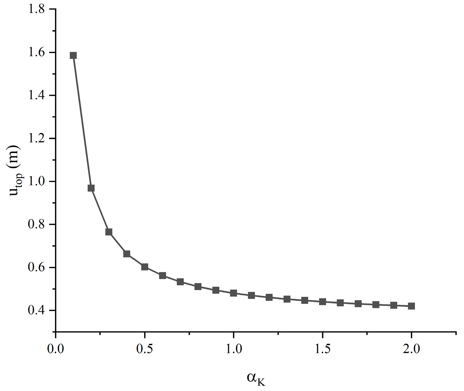
4.3. Dynamic Foundation Impedance

As shown in Figure 15, with increasing load frequency, the change of horizonal foundation impedance is not obvious. When the load frequency is around soil cut-off frequency, the horizontal foundation impedance slightly decreases. The foundation impedance is very sensitive to the pile length submerged in the seawater. With an increasing pile embedment ratio, the foundation impedance decreases significantly.

Meanwhile, the wave load can influence the foundation impedance to a certain degree. As shown in Figure 16, when the wave load is relatively small (wavelength $L_{wl}=75\mathrm{m}$, wave height $H_w=4\mathrm{m}$), the influence of wave load on the foundation impedance is not significant. When the wave load is relatively large (wavelength $L_{wl}=120\mathrm{m}$, wave height $H_w=8\mathrm{m}$), the influence of wave load on the foundation impedance is significant.

5. Conclusions

This paper establishes the model of pile group supported OWT under wind and wave load; the main findings are presented below:

(1)

With increasing wind speed, the tower displacement increases significantly. The influence of foundation impedance on the tower displacement is more significant when the foundation impedance is relatively small.

(2)

The pile–pile interaction factor depends largely on the pile spacing. When the pile spacing is large, the influence of the passive pile on the active pile can be ignored; when the pile spacing is small, a secondary wave effect should be considered for the pile–pile interaction factor.

(3)

When the pile embedded ratio is large, the pile–pile interaction is more obvious. When the incidence angle is $45°$, the pile–pile interaction is less significant compared with that of $0°$ and $90°$.

(4)

The foundation impedance decreases significantly with an increasing pile embedment ratio.

(5)

The influence of wave load on the foundation impedance is more obvious when the wave load is large.

References

1. Feyzollahzadeh, M.; Mahmoodi, M.; Yadavar-Nikravesh, S.; Jamali, J. Wind load response of offshore wind turbine tow-ers with fixed monopile platform. J. Wind Eng. Ind. Aerodyn. 2016, 158, 122–138. [Google Scholar] [CrossRef]
2. Zheng, X.Y.; Li, H.; Rong, W.; Li, W. Joint earthquake and wave action on the monopile wind turbine foundation: An experimental study. Mar. Struct. 2015, 44, 125–141. [Google Scholar] [CrossRef] [Green Version]
3. Gupta, B.K.; Basu, D. Offshore wind turbine monopile foundations: Design perspectives. Ocean Eng. 2020, 213, 107514. [Google Scholar] [CrossRef]
4. Bhattacharya, S. Challenges in Design of Foundations for Offshore Wind Turbines. Eng. Technol. Ref. 2014, 1, 922. [Google Scholar] [CrossRef]
5. Lombardi, D.; Bhattacharya, S.; Wood, D.M. Dynamic soil–structure interaction of monopile supported wind turbines in cohesive soil. Soil Dyn. Earthq. Eng. 2013, 49, 165–180. [Google Scholar] [CrossRef]
6. Damgaard, M.; Bayat, M.; Andersen, L.; Ibsen, L. Assessment of the dynamic behaviour of saturated soil subjected to cyclic loading from offshore monopile wind turbine foundations. Comput. Geotech. 2014, 61, 116–126. [Google Scholar] [CrossRef]
7. Bouzid, D.A.; Bhattacharya, S.; Otsmane, L. Assessment of natural frequency of installed offshore wind turbines using nonlinear finite element model considering soil-monopile interaction. J. Rock Mech. Geotech. Eng. 2018, 10, 333–346. [Google Scholar] [CrossRef]
8. Alkhoury, P.; Soubra, A.H.; Rey, V.; Aït-Ahmed, M. A full three-dimensional model for the estimation of the natural fre-quencies of an offshore wind turbine in sand. Wind Energy 2021, 24, 699–719. [Google Scholar] [CrossRef]
9. Kjørlaug, R.A.; Kaynia, A.M. Vertical earthquake response of megawatt-sized wind turbine with soil-structure interaction effects. Earthq. Eng. Struct. Dyn. 2015, 44, 2341–2358. [Google Scholar] [CrossRef]
10. Corciulo, S.; Zanoli, O.; Pisanò, F. Transient response of offshore wind turbines on monopiles in sand: Role of cyclic hy-dro–mechanical soil behaviour. Comput. Geotech. 2017, 83, 221–238. [Google Scholar] [CrossRef] [Green Version]
11. Zuo, H.; Bi, K.; Hao, H. Dynamic analyses of operating offshore wind turbines including soil-structure interaction. Eng. Struct. 2018, 157, 42–62. [Google Scholar] [CrossRef]
12. Galvín, P.; Romero, A.; Solís, M.; Domínguez, J. Dynamic characterisation of wind turbine towers account for a monopile foundation and different soil conditions. Struct. Infrastruct. Eng. 2017, 13, 942–954. [Google Scholar] [CrossRef]
13. Kausel, E. Early history of soil–structure interaction. Soil Dyn. Earthq. Eng. 2010, 30, 822–832. [Google Scholar] [CrossRef] [Green Version]
14. Reese, L.C. Non-dimensional solutions for laterally loaded piles with soil modulus assumed proportional to depth. In Proceedings of the 8th Texas Conference on Soil Mechanics and Foundation Engineering, Austin, TX, USA, 14–15 September 1956. [Google Scholar]
15. McClelland, B.; Focht, J. Soil modulus for laterally loaded piles. J. Soil Mech. Found. Div. 1956, 82, 1081-1–1081-22. [Google Scholar] [CrossRef]
16. Darvishi-Alamouti, S.; Bahaari, M.R.; Moradi, M. Natural frequency of offshore wind turbines on rigid and flexible monopiles in cohesionless soils with linear stiffness distribution. Appl. Ocean Res. 2017, 68, 91–102. [Google Scholar] [CrossRef]
17. Andersen, L.V.; Vahdatirad, M.; Sichani, M.T.; Sørensen, J.D. Natural frequencies of wind turbines on monopile founda-tions in clayey soils—A probabilistic approach. Comput. Geotech. 2012, 43, 1–11. [Google Scholar] [CrossRef]
18. Adhikari, S.; Bhattacharya, S. Vibrations of wind-turbines considering soil-structure interaction. Wind Struct. Int. J. 2011, 14, 85–112. [Google Scholar] [CrossRef] [Green Version]
19. Adhikari, S.; Bhattacharya, S. Dynamic Analysis of Wind Turbine Towers on Flexible Foundations. Shock Vib. 2012, 19, 37–56. [Google Scholar] [CrossRef]
20. Bhattacharya, S.; Adhikari, S. Experimental validation of soil–structure interaction of offshore wind turbines. Soil Dyn. Earthq. Eng. 2011, 31, 805–816. [Google Scholar] [CrossRef]
21. Nogami, T.; Paulson, S.K. Transfer matrix approach for nonlinear pile group response analysis. Int. J. Numer. Anal. Methods Geomech. 1985, 9, 299–316. [Google Scholar] [CrossRef]
22. Zhang, L.; Gong, X.-N.; Yang, Z.-X.; Yu, J.-L. Elastoplastic solutions for single piles under combined vertical and lateral loads. J. Cent. South Univ. Technol. 2011, 18, 216–222. [Google Scholar] [CrossRef]
23. Zhang, L.; Zhao, M.; Zou, X. Behavior of Laterally Loaded Piles in Multilayered Soils. Int. J. Géoméch. 2015, 15, 06014017. [Google Scholar] [CrossRef]
24. Wang, M.; Wang, Z.; Zhao, H. Analysis of Wind-Turbine Steel Tower by Transfer Matrix. In Proceedings of the 2009 International Conference on Energy and Environment Technology, Guilin, China, 16–18 October 2009. [Google Scholar]
25. Huang, M.; Zhong, R. Coupled horizontal-rocking vibration pf partially embedded pile groups and its effect on resonance of offshore wind turbine structures. Chinsese J. Geotech. Eng. 2014, 36, 286–294. [Google Scholar]
26. Anoyatis, G.; Mylonakis, G.; Lemnitzer, A. Soil reaction to lateral harmonic pile motion. Soil Dyn. Earthq. Eng. 2016, 87, 164–179. [Google Scholar] [CrossRef] [Green Version]
27. Anoyatis, G.; Lemnitzer, A. Dynamic pile impedances for laterally–loaded piles using improved Tajimi and Winkler for-mulations. Soil Dyn. Earthq. Eng. 2017, 92, 279–297. [Google Scholar] [CrossRef] [Green Version]
28. Shuqing, W.; Bingchen, L. Wave Mechanics for Ocean Engineering; China Ocean University Press: Qingdao, China, 2013. (In Chinese) [Google Scholar]
29. Xin-xin, L.; Da-peng, S.; Xue-jiao, X.; Hao, W.; Yu-cheng, L. Experimental study of irregular wave force loads on high rise pile platform. J. Waterw. Harb. 2013, 34, 277–284. (In Chinese) [Google Scholar]
30. Dobry, R.; Gazetas, G. Dynamic Response of Arbitrarily Shaped Foundations. J. Geotech. Eng. 1986, 112, 109–135. [Google Scholar] [CrossRef]
31. Mylonakis, G.; Gazetas, G. Lateral Vibration and Internal Forces of Grouped Piles in Layered Soil. J. Geotech. Geoenvironmental Eng. 1999, 125, 16–25. [Google Scholar] [CrossRef]
32. Luan, L.; Zheng, C.; Kouretzis, G.; Ding, X. Dynamic analysis of pile groups subjected to horizontal loads considering coupled pile-to-pile interaction. Comput. Geotech. 2020, 117, 103276. [Google Scholar] [CrossRef]
33. Van Binh, L.; Ishihara, T.; Van Phuc, P.; Fujino, Y. A peak factor for non-Gaussian response analysis of wind turbine tower. J. Wind Eng. Ind. Aerodyn. 2008, 96, 2217–2227. [Google Scholar] [CrossRef]
34. Veritas, N. Environmental Conditions and Environmental Loads; Det Norske Veritas Oslo: Høvik, Norway, 2000. [Google Scholar]
35. Jara, F.A.V. Model Testing of Foundations for Offshore Wind Turbines; Oxford University: Oxford, UK, 2006. [Google Scholar]
36. Kaynia, A.M. Dynamic Stiffness and Seismic Response of Pile Groups; Massachusetts Institute of Technology: Cambridge, MA, USA, 1982. [Google Scholar]
Figure 1. Frequency spectrum of the dynamic loads [4].
Jmse 10 01024 g001
Figure 2. Pile group supported 3.6 MW offshore wind turbine.
Jmse 10 01024 g002
Figure 3. Pile–pile interaction.
Jmse 10 01024 g003
Figure 4. Pile–pile interaction.
Jmse 10 01024 g004
Figure 5. Thrust coefficient C T -tip speed ratio λ s curve [35].
Jmse 10 01024 g005
Figure 6. Tower discretization.
Jmse 10 01024 g006
Figure 7. FEM numerical simulation model.
Jmse 10 01024 g007
Figure 8. Meshing of the model.
Jmse 10 01024 g008
Figure 9. Comparison between the calculation result and FEM result.
Jmse 10 01024 g009
Figure 10. The influence of the wind speed on the tower displacement.
Jmse 10 01024 g010
Figure 11. The influence of the foundation impedance on the tower displacement.
Jmse 10 01024 g011
Figure 12. Pile–pile interaction under different pile spacings.
Jmse 10 01024 g012
Figure 13. Pile–pile interaction under different pile embedded ratios.
Jmse 10 01024 g013
Figure 14. Pile–pile interaction under different incidence angles.
Jmse 10 01024 g014
Figure 15. The influence of the pile length in seawater on the foundation impedance.
Jmse 10 01024 g015
Figure 16. The influence of the wave load on the foundation impedance.
Jmse 10 01024 g016