Dynamic Response of a Four-Pile Group Foundation in Liquefiable Soil Considering Nonlinear Soil-Pile Interaction

Abstract

Piles, which are always exposed to dynamic loads, are widely used in offshore structures. The dynamic response of the pile-soil-superstructure system in liquefiable soils is complicated, and the interaction between the pile and soil and the pile volume effect are the key influencing factors. In this study, a water-soil fully coupled dynamic finite element-finite difference (FE-FD) method was used to numerically simulate the centrifuge shaking table (CST) test of a four-pile group in saturated sand soil. An interface contact model was proposed to simulate the pile-soil interaction, and a solid element was used to consider the volume effect of the pile. The acceleration responses of the soil and pile, settlement deformation, excess pore water pressure, and bending moment were examined. The results show that the bending moment response of the two piles parallel to the shaking direction show minor differences, while the two piles perpendicular to the shaking direction show almost the same distribution. The values of excess pore water pressure at the same depth but different azimuth angles around the pile are also different. The numerical simulation can accurately reproduce soil deformation and pile internal force during and after dynamic loading.

1. Introduction

Piles are widely used in marine engineering, for the establishment of structures such as offshore wind turbines, offshore drilling platforms, and bridges. Piles are always exposed to a variety of external dynamic loads, such as wind, waves, and earthquakes [1,2]. Piles usually work in the form of closely spaced pile groups that bear the load transmitted by their caps. In addition, each pile is also affected by the load of the adjacent pile, which is called the dynamic pile group effect [3,4,5]. The response of a single pile within a pile group differs from that of an isolated pile. Large-scale shaking table tests performed using a pile group in dry sand layers reveal that soil deformation in the vicinity of piles is the key factor influencing group effects during earthquakes [5]. Centrifuge test results have also shown that the bending moment distribution of single pile in a group is a function of the pile position and excitation frequency. Furthermore, inner piles have the greatest kinematic bending moment, whereas outer piles have more pronounced inertial counterparts [6]. The group effect increases with an increase in the relative displacement between the soil and piles [7,8]. Therefore, it is unreasonable to directly apply the research results for single piles to pile groups.

Extensive research has been conducted on pile-group foundations [4,9,10,11,12,13]. The interaction between the pile and the surrounding soil usually includes one or more pile-soil interactions (PSI), pile cap-pile interactions (CPI), cap-soil interactions (CSI), and pile-pile interactions (PPI) [14,15,16,17,18,19]. More attention has been paid to pile-soil interactions (PSI). Specifically, pile-soil interface separation was investigated [9,15], where the behaviour of soil around the pile was nonlinear under dynamic conditions, and the soil around the pile heads generated a large internal force, causing separation between the soil and pile under dynamic conditions. Moreover, the soil around the pile was not only separated, but its contact behaviour was nonlinear when subjected to strong earthquakes.

Correctly defined kinematic pile-soil interface elements are essential for improving the prediction accuracy of pile-soil interactions. Determination of the pile-soil interface has been extensively studied. However, there is no consensus on an optimal constitutive model of interface elements with sufficient accuracy and mathematical simplicity. Idealised models have been used for interface elements, but important physical mechanisms should not be neglected [17], especially in liquefiable soil, where earthquakes often cause pile foundation failure [20]. Motamed et al. [21] studied a pile group subjected to large liquefaction-induced ground displacements and discussed the effects of lateral spreading on the pile group. The higher excess pore water pressure developed in the sand reduced the bearing capacity of the pile, and the shaft resistance was reduced significantly as the thickness of the liquefiable sand layer increased [22]. Lee et al. [3] performed a 3-D finite element (FE) analysis of pile groups that considered the influence of soil slippage but did not consider the influence of cap fixing and superstructure load. However, when dealing with the pile-soil interaction problem of dynamic excitation, a complete system model consisting of a stratum, foundation, and superstructure should be established for the analysis [23].

Studies of the performance of pile foundations during past earthquakes have shown that excessive settlement of piles during soil liquefaction was a significant factor in the failure of supported structures. In addition, liquefied soil may experience high strains because of the densification process during the build-up of excess pore pressure [24,25]. Thus, the bearing capacity of the soil and foundation may decrease, leading to excessive settlement, and compromising the serviceability and integrity of the structure [22,26]. However, attention should be given to the pile response after ground motion because large soil deformation can cause severe residual strain and internal force to piles during pore water dissipation. In contrast to previous studies that regarded the pile-soil interface as a displacement continuity boundary or general static Coulomb friction contact, Bao et al. proposed a connection element with a hard and soft contact definition to simulate the behaviour of the pile-soil interface [27]. However, the simulation was on a single pile. A pile-group simulation should be examined as well.

In this study, the finite element-finite difference (FE-FD) method was used to study the dynamic response of a four-pile group foundation with a superstructure load in liquefied soil during and after dynamic excitation considering the influence of the pile-soil interface parameters. The mechanical behaviour of soil is described by an elastoplastic constitutive model that considers the characteristics of the structure, excessive consolidation of the soil, and anisotropy caused by stress. The calculated results were compared with data from the centrifuge shaking table (CST) test. The main purpose of this study was to provide a reasonable numerical method for simulating the dynamic response of a group pile-soil system that considers the load of the superstructure. Special attention should be paid to the behaviour of piles after loading, when a large residual stress may occur.

2. Numerical Analysis Model

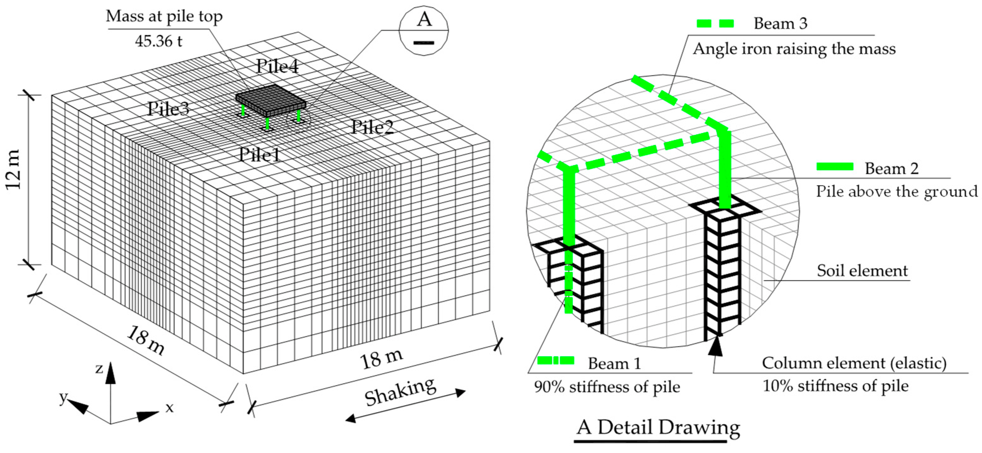
2.1. Finite Element Model

Figure 1 shows the three-dimensional FE model proposed based on the CST test, which is introduced in the next section. According to the similarity law, the size of the analysis domain was 18 m (length) × 18 m (width) × 12 m (height). The foundation was a group of four aluminum pipe piles with a length of 10.1 m and diameter of 0.57 m located in the center of the domain. The wall thickness of the pipe was 0.096 m, and 9 m of the pipe was buried in the soil. In addition, the centre distance between the piles was 2.28 m. The size of the footing on the pile top was 2.85 m (length) × 2.85 m (width) × 0.3 m (height), and a weight of 45,360 kg was used to simulate the load from the superstructure. In the FE model, the soil was simulated using solid elements, and the pile was simulated using a hybrid element composed of beam and column elements. Each beam element was surrounded by four column elements to consider the volume of the pile. Horizontal beams were also used to simulate the connection between the piles at the top through the footing. To analyse the response of the pile in different locations of the pile group, where piles 1 and 2 are parallel to the shaking direction, and are called the front pile and back pile, respectively, according to the shaking direction. Piles 1 and 3 are perpendicular to the shaking direction and are called parallel piles with united movement.

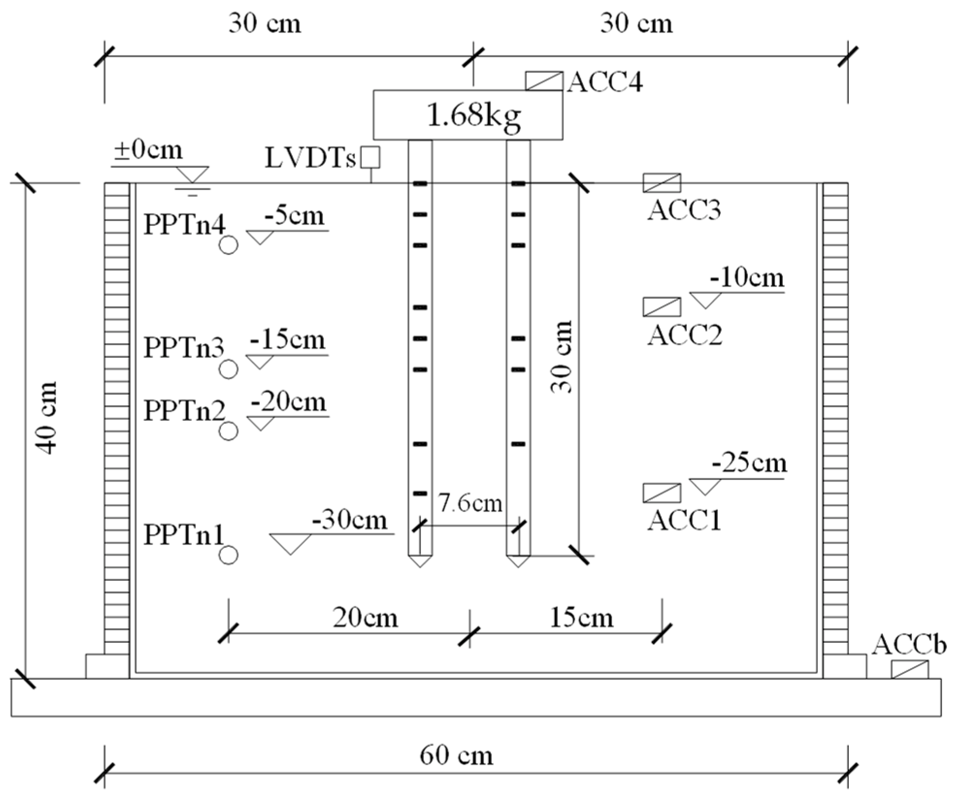
2.2. Centrifuge Shaking Table Test on Group Piles

A series of CST tests was conducted on piles in saturated sand under dynamic loads to verify the numerical model proposed in this study. The CST test used a laminar box, which was approximately circular, in a 12-sided shape with a diameter of 60 cm and a height of 40 cm. The wall of the box was made of light aluminium alloy, and the single ring was 8.9 mm high. A certain degree of relative displacement could occur between adjacent rings, reducing the influence of the boundary effect during ground vibration. Standard Toyoura sand was used to make the saturated ground, with a maximum porosity ratio e_max = 0.977, a minimum porosity ratio e_min = 0.597, and an initial ground permeability coefficient k = 2 × 10⁻⁴ m/s.

As shown in Figure 2, the piles in the test were thin-walled hollow square aluminium pipes made of an aluminium alloy. A group of four piles with connections at the top was buried in the middle of the saturated sand. The top of the piles was 3.5 cm above the soil surface and was fixed with a concentrated mass of 1.68 kg to simulate the superstructure. Furthermore, 30 cm of the pile was buried below the soil surface. The parameters of the piles are presented in

Table 1. Parameters of model pile and corresponding prototype (satisfying scaling law).

Parameters		Model Type in Test	Prototype in Simulation
Gravity Field (g)		30	1
Model box size (m)		Diameter × height 0.6 × 0.4	length × width × height 18 × 18 × 12
Aluminum pipe pile	Yield stress (MPa)	290	290
	Young’s modulus, E (GPa)	70	70
	Section size (m)	0.19 × 0.19	0.57 × 0.57
	Thickness (m)	3.2 × 10−3	9.6 × 10−2
	Area (m2)	2.02 × 10−4	0.182
	Moment of inertia Ix (m4)	8.8 × 10−9	7.1 × 10−3
	Poisson’s ratio, ν	0.3	0.3
Mass at pile top (kg)		1.68	45360

. The piles and soil were subjected to vibration loading in an environment with a centrifugal acceleration of 30 g, and the parameters of input excitation in the model type and corresponding prototype in simulation are listed in

Table 2. Input dynamic wave in model type and prototype (satisfying scaling law).

Type	Peak Ground Acceleration, Ap	Time, T	Frequency, f
Centrifuge experiment (model type)	3.80 g	0.6 s	50 Hz
Numerical analysis (prototype)	0.13 g	18 s	1.67 Hz

.

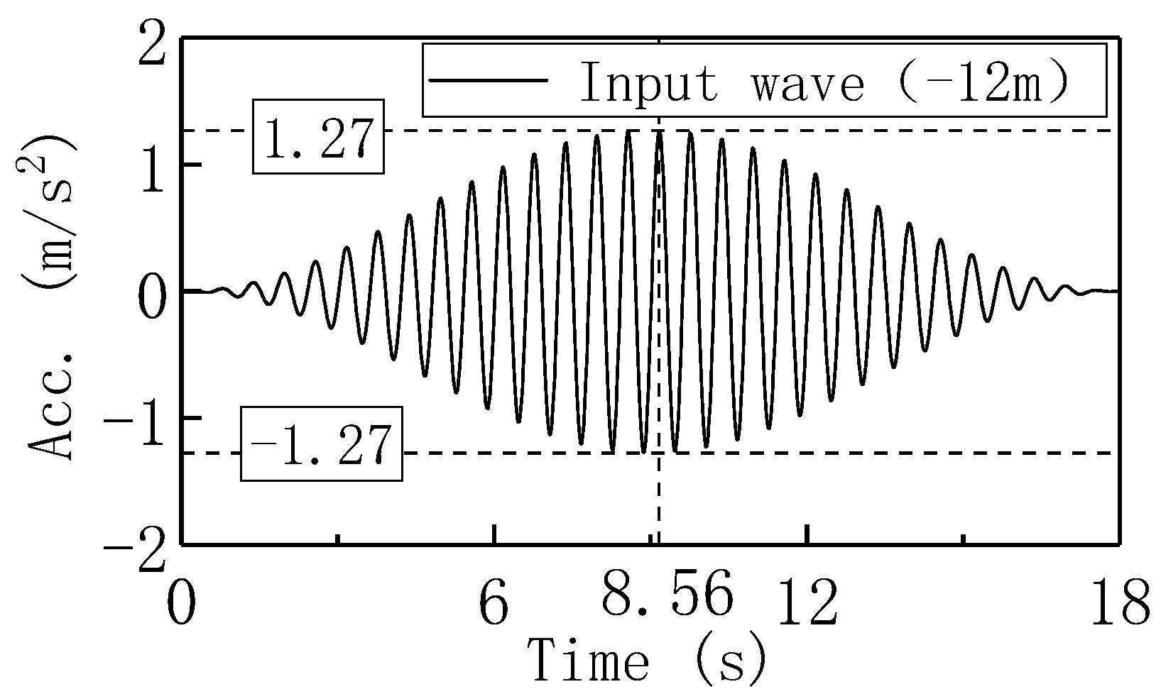
2.3. Input Dynamic Load

The input dynamic load is shown in Figure 3, and the parameters of the dynamic wave in model tests and prototype used in the simulation are listed in Table 2. The dynamic load is used to analyse the behaviour at random frequencies, which was obtained from the CST test according to a similar ratio, and the time interval of the input wave was 0.02 s. Excitation acceleration was applied to the bottom of the foundation model along the horizontal direction (Figure 1).

2.4. Soil Constitutive Model

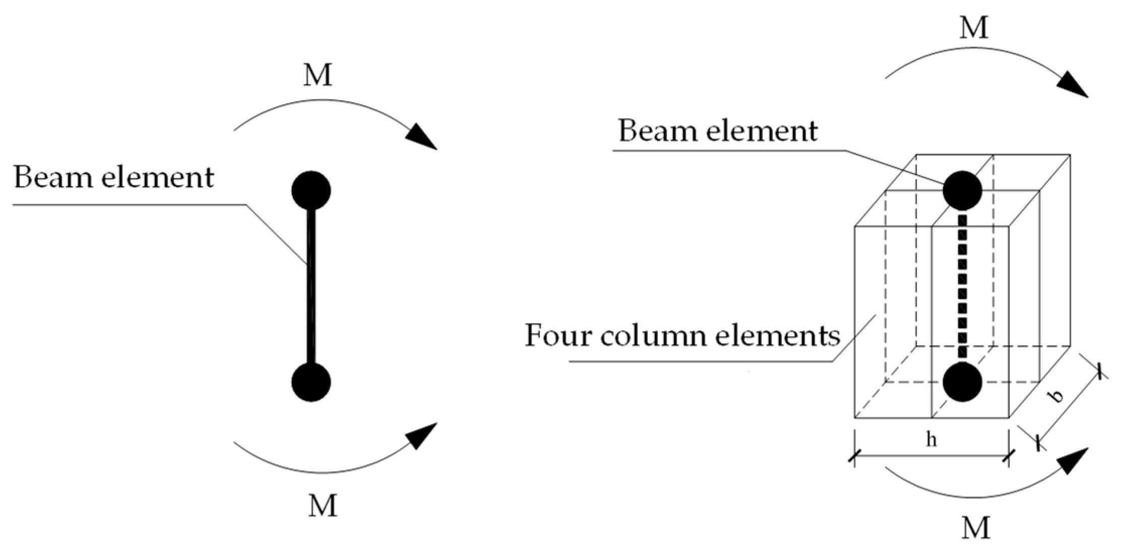
It is important to choose an appropriate constitutive model when solving dynamic pile-soil nonlinear problems. Under drained and undrained conditions, the model should be able to describe the liquefaction behaviour of saturated soil under cyclic loading. Therefore, the cyclic mobility (CM) model proposed by Zhang et al. [28] was used in the numerical analysis. One of the remarkable features of this model is that it can show the evolution of the soil condition, including over-consolidation, changes in the structure, and stress-induced soil anisotropy during dynamic loading. The CM model has eight control parameters, among which, five parameters, R_f, λ, κ, e_N and ν, are the same as those in the modified Cam-clay model, while the other three parameters, m_R, m_R* and br, reflect the evolution of over-consolidation, structure degradation, and the development of anisotropy, respectively, when the soil is subjected to alternating loading under various drainage conditions. The determination of the parameters of the CM model and verification of the model can be found in references [28,29,30]. The constitutive and initial state parameters of the Toyoura sand used in this study are listed in

Table 3. Parameters of Toyoura sand in CM model used for calculation.

Parameters	Value
Critical ratio of principal stress, Rf	3.14
Compression index, λ	0.05
Swelling index, κ	0.008
Reference void ratio, eN (p’ = 98 kPa)	0.87
Poisson’s ratio, ν	0.30
Degradation parameter of over-consolidation, mR	0.10
Degradation parameter of structure, mR*	2.20
Evolution parameter of anisotropy, br	1.50
Initial void ratio, e0	0.825
Initial degree of structure, R0*	0.95
Initial anisotropy, ζ0	0

. The unit weight of the saturated sand was 19 kN/m³, and the relative density was Dr = 40% (loose sand) when preparing the CST test. Rayleigh damping was used for dynamic wave attenuation in the soil.

2.5. Pile Model

The piles buried in the soil were modelled by beam elements with surrounding column elements, whereas the parts of the piles above the soil surface and the horizontal connecting beams at the top of the piles were simulated by elastic beam elements (Figure 4). The role of the beam element is to consider the main stiffness of the pile in the dynamic calculation, whereas the column element, which is an eight-node solid element, considers the volume effect of the pile. The basic parameters of the connecting beam and mass at the top of the pile are listed in

Table 4. Physical parameters of connection beam at pile top and mass.

Type	Parameters	Model Type in CST Test	Prototype in Calculation
Connection beam atpile top	Size (mm)	30 × 30 × 4	900 × 900 × 120
	Area (cm2)	2.236	2010
	Moment of inertia Ix (cm4)	1.77 × 10−2	1.43 × 106
Mass at pile top	Mass (kg)	0.42 × 4 = 1.68	45,360

, and the calculation parameters of the pile model are listed in

Table 5. Material parameters of pile used for calculation.

Elements	Parameters	Units	Beam 1	Beam 2	Beam 3
Beam element	E	kPa	6.3 × 107	7.0 × 107	7.0 × 107
	ν	1	0.20	0.20	0.20
	A	m2	0.182	0.182	0.201
	Ix and Iy	m4	7.1 × 10−3	7.1 × 10−3	1.43 × 10−2
	ρ	kg/m3	7.8 × 103	7.8 × 103	1.43 × 10−2
Column element	E	kPa	5.65 × 106	-	-
	ν	1	0.20
	ρ	kg/m3	0
Pile side joint element	Kn1	kN/m3	7 × 107	-	-
	Ks1	kN/m3	3
	σt1	kPa	−1 × 109
	vcm1	M	−1
	C1	kPa	0
	φ1	1	15°
Pile bottom joint element	Kn2	kN/m3	7 × 107	-	-
	Ks2	kN/m3	1 × 102
	σt2	kPa	−1 × 109
	vcm2	M	−1
	C2	kPa	0
	φ2	1	15°

. In summary, there are 10,784 soil elements, 88 beam elements, 200 elastic solid elements (simulating the footing at the top of the piles), 144 column elements, and 400 joint elements (simulating the interface between the soil and pile) in the FE model.

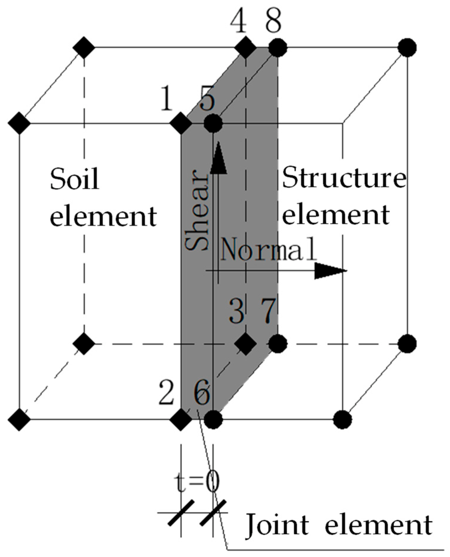
2.6. Pile-Soil Interface

As detailed in the previous study [27], the joint element existing between the column element and the soil element was used to represent the pile-soil contact (Figure 5). The joint element is an eight-node zero-thickness contact element, in which four nodes on one side share nodes with the soil element, and four nodes on the other side share nodes with the column element of the pile (or underground structure). It forms four sets of node pairs: nodes 1 and 5, nodes 2 and 6, nodes 3 and 7, and nodes 4 and 8, where the initial coordinates of each node pair are the same. For the joint elements, it is assumed that the normal and tangential stiffnesses are independent of each other. This not only describes the elastic extrusion and elastoplastic slippage between two different materials on the contact surface, but also considers the separation (stiffness failure) of the contact surface and re-contact (stiffness recovery). Figure 6 shows the relationship between the stress and strain for joint elements in which the pressure is positive and the tension is negative. The behaviour of the joint element can be described as follows.

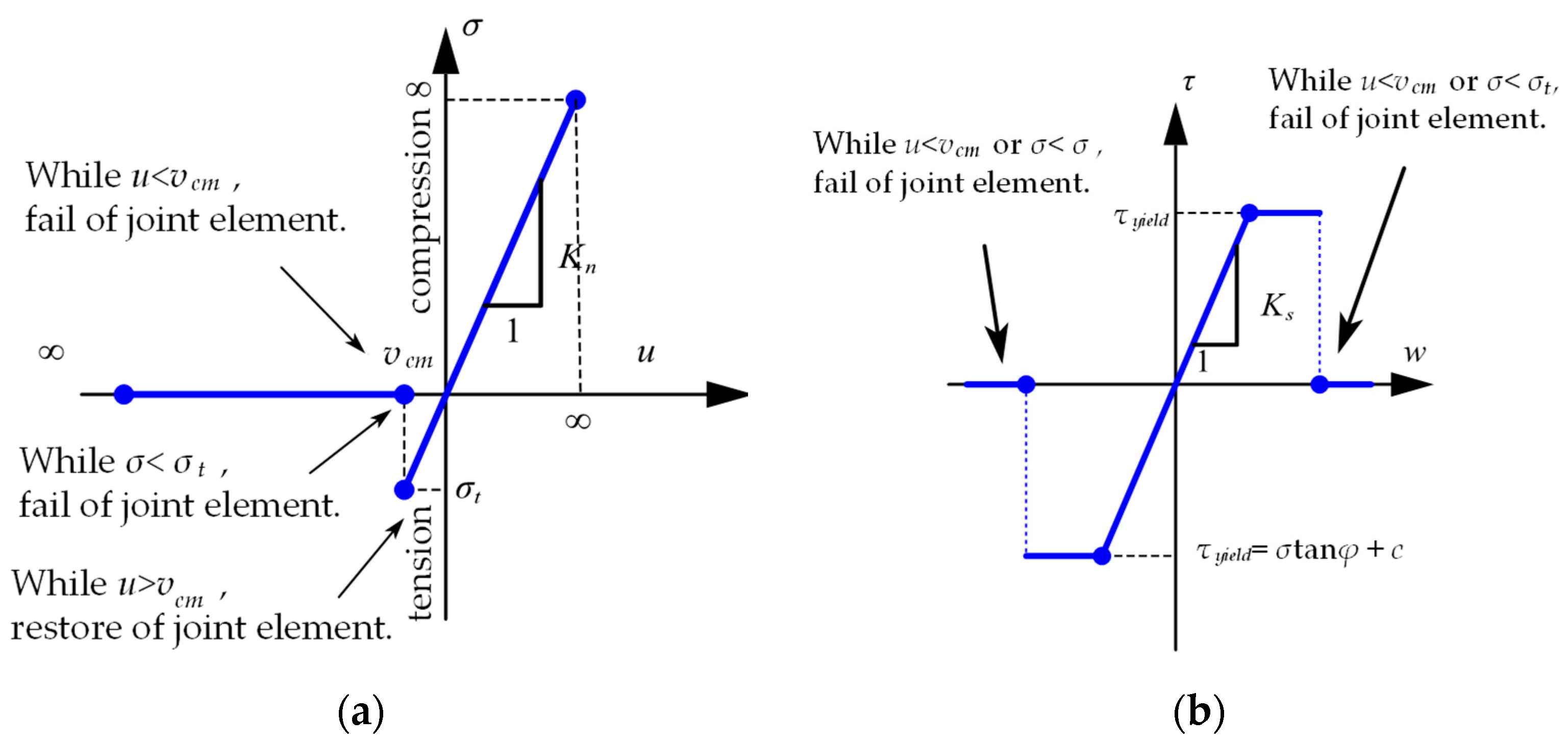
• In the elastic stage, before the joint element fails, it exhibits elastic behaviour in the normal and tangential directions (Figure 6a), and the normal stress-displacement relationship follows (1):

  τ = ω · K_s

  (1)

  where w is the tangential displacement, and K_s is the tangential stiffness coefficient.
• In the fully plastic stage, the yield stress of the joint element follows the Mohr-Coulomb theory (2),

  |τ_yield| = | σ | tan φ + c

  (2)

  where φ is the effective internal friction angle; c is the soil cohesion; σ is the normal effective stress of the joint elements, which is the total stress minus the pore water pressure.
• Assuming that the critical value of the normal displacement u of the joint element is v_cm, when u > v_cm (Figure 6a) or |u| < |v_cm| (Figure 6b), both the normal and tangential stiffnesses of the joint element are restored.

2.7. Boundary Conditions

The water-soil coupling program DBLEAVES [31], based on the effective stress framework, was used for the calculation. The “u-p” form field equations for solid phase and liquid phase were solved through the FE-FD method, and the Newmark β method was adopted in the time domain. The program of the water-soil-coupling method was verified through a series of dynamic and static analyses of the soil-foundation superstructure; the details can be found in references [10,22,23,32].

Equal displacement boundary conditions in the x direction and y direction were set on the two boundary surfaces. The displacements of the nodes at the bottom boundary were all fixed, whereas the top surface was set as a free boundary. Except for the top surface, which was considered as the drainage boundary, the other boundaries were all non-drained boundaries. According to this definition, the permeability coefficient k₀ is determined by (3).

$$k_0=K\frac{\rho \mathrm{g}}{\eta }$$

(3)

where k₀ is the initial permeability coefficient, K is the permeability of the porous medium, which generally depends on the particle gradation and pore distribution of the soil, ρ is the density of the fluid, η is the dynamic viscosity coefficient of the fluid, g is the acceleration due to gravity.

In the CST test, the gravitational acceleration magnification is N = 30 g, and theoretically, the permeability coefficient k₀ is 30 times the magnification, according to (3). The physical process of seepage in CST tests is complex. Arulanandan et al. [33] found that when sand was liquefied, the contact between soil particles gradually disappeared, which provided a channel for the seepage of pore water and proposed that the permeability coefficient started to change. At the liquefaction stage, the permeability coefficient increased to 6.7 times of the initial k₀ and then decreased to close to k₀ after pore pressure dissipation. Shahir et al. [34] assumed that the permeability coefficient increased and decreased as the pore water pressure ratio accumulated and dissipated. In the three-dimensional water-soil fully coupled dynamic calculation, the permeability coefficient k was valued eight times that of the initial k₀ based on the fitting data of the permeability coefficient from the CST model test [35].

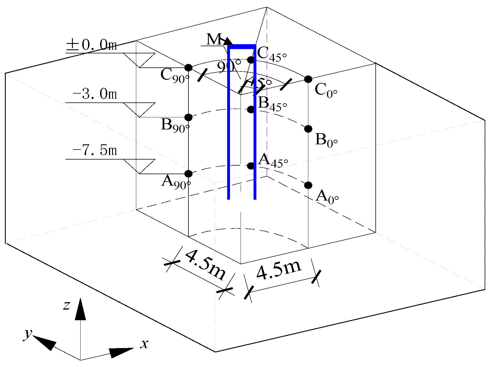
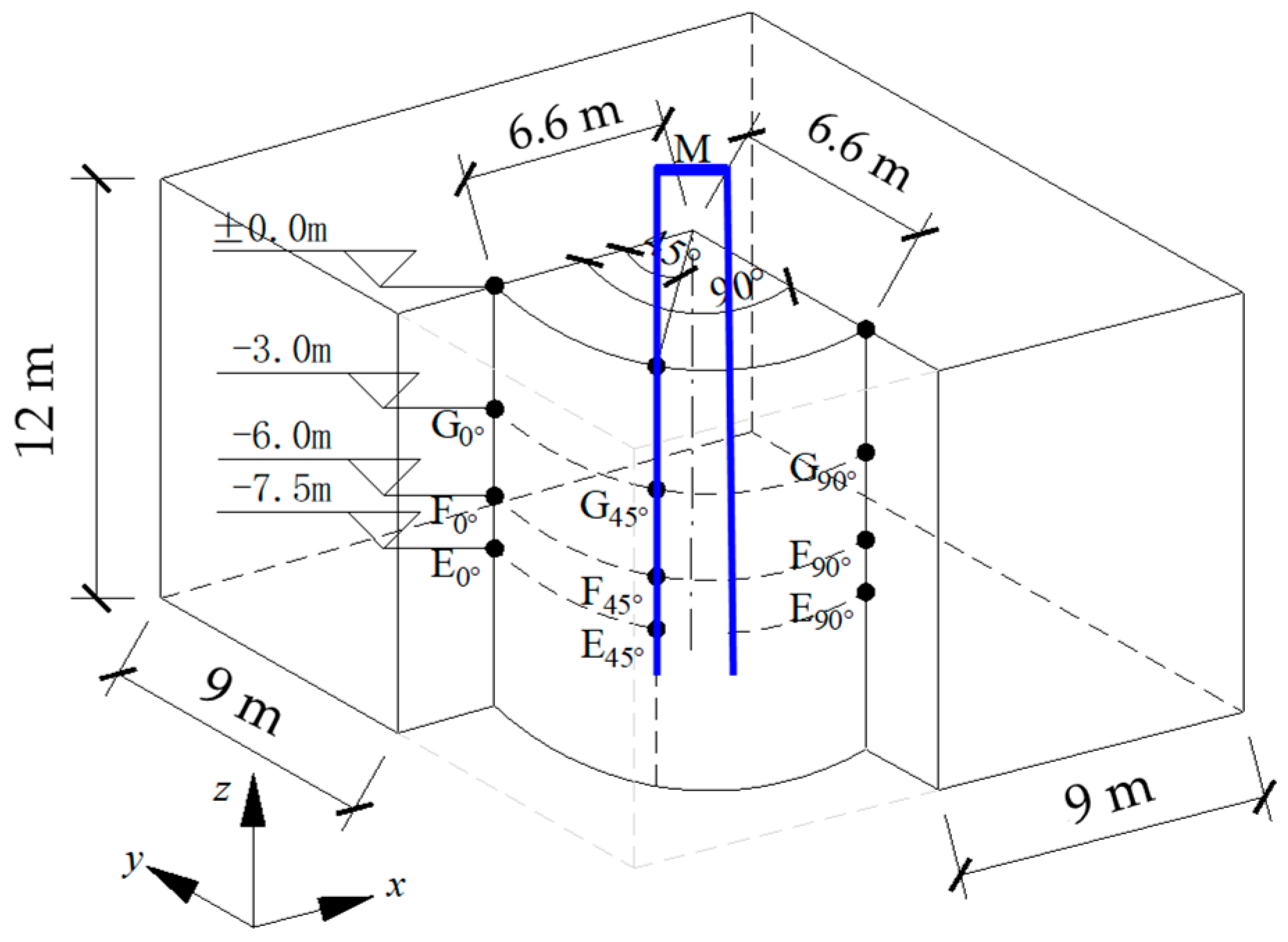
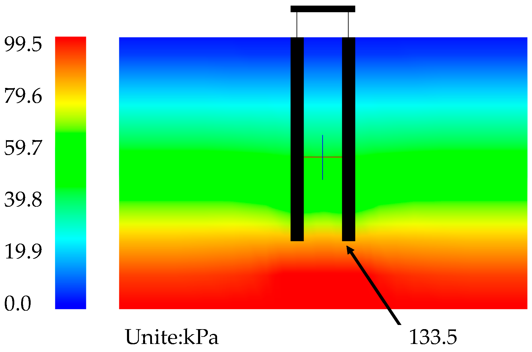
2.8. Observation Points and Initial Effective Stress in Soil

In the numerical analysis, the observation points for acceleration and excess pore water pressure in the soil are shown in Figure 7 and Figure 8, respectively. The observation points A90°, B90°, C90°, E45°, F45°, and G45° corresponded to the measuring points in the CST test at different depths. Point M indicates the position at the top of the pile. The test data were converted into a prototype according to the similarity law when comparing the results of the numerical analysis and CST test.

A static calculation was performed to obtain the initial ground stress field. At the same time, the influence of the piling process on the stress field was ignored. The distribution of effective stress σ_y in the vertical direction of the ground is shown in Figure 9. From the stress contour, it can be observed that the stress of the soil element is distributed in the layer, and the effective stress of the bottom element is 99.5 kPa. Owing to the gravity of the mass at the pile top, the maximum effective stress of the soil element close to the bottom of the pile reached 133.5 kPa.

3. Results and Discussion

3.1. Dynamic Response of Soil

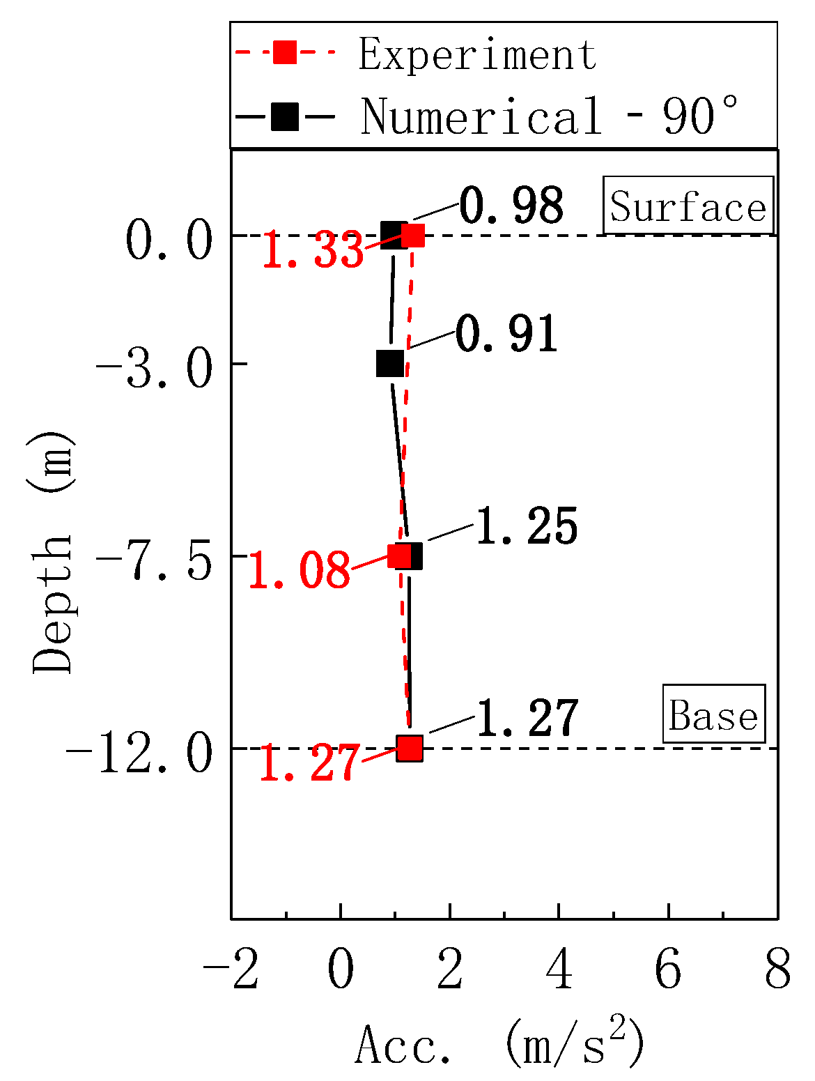
3.1.1. Acceleration Response

The arrangement of the acceleration measurement points is shown in Figure 7. As shown in Figure 10, time history of input dynamic wave, the peak acceleration of the input wave (1.27 m/s²) appears at 8.56 s. From the numerical simulation results, it can be observed that the peak acceleration of A90° is slightly lower than that of the experimental results; it is 1.25 m/s² and appears at 8.62 s; the peak acceleration of B90° further decreases (0.91 m/s²) and appears at 8.76 s. This indicates that although the acceleration in the soil has decreased, the magnitude does not attenuate significantly. Liquefaction does not occur in the soil at depth of −7.5 m~−3.0 m; the peak surface acceleration of C90° (0.98 m/s²) is slightly larger than the soil acceleration at −3 m and appears at 7.1 s (about 2 s earlier than at −3 m). After 7.1 s, the acceleration at C90° on the soil surface has a relatively obvious trend of attenuation and “shrinkage”, which indicates that the shallow soil layer of −3 m to 0 m may have liquefied to a large degree. The peak acceleration at the superstructure mass was 1.55 m/s², and there was no obvious relative attenuation. Figure 11 compares the acceleration values in the soil at different depths between the numerical simulation and the CST test (90° angle). Although the surface acceleration (1.33 m/s²) of the CST test is slightly larger than the numerical simulation result (0.982 m/s²), their trends are the same; the acceleration does not change significantly with depth.

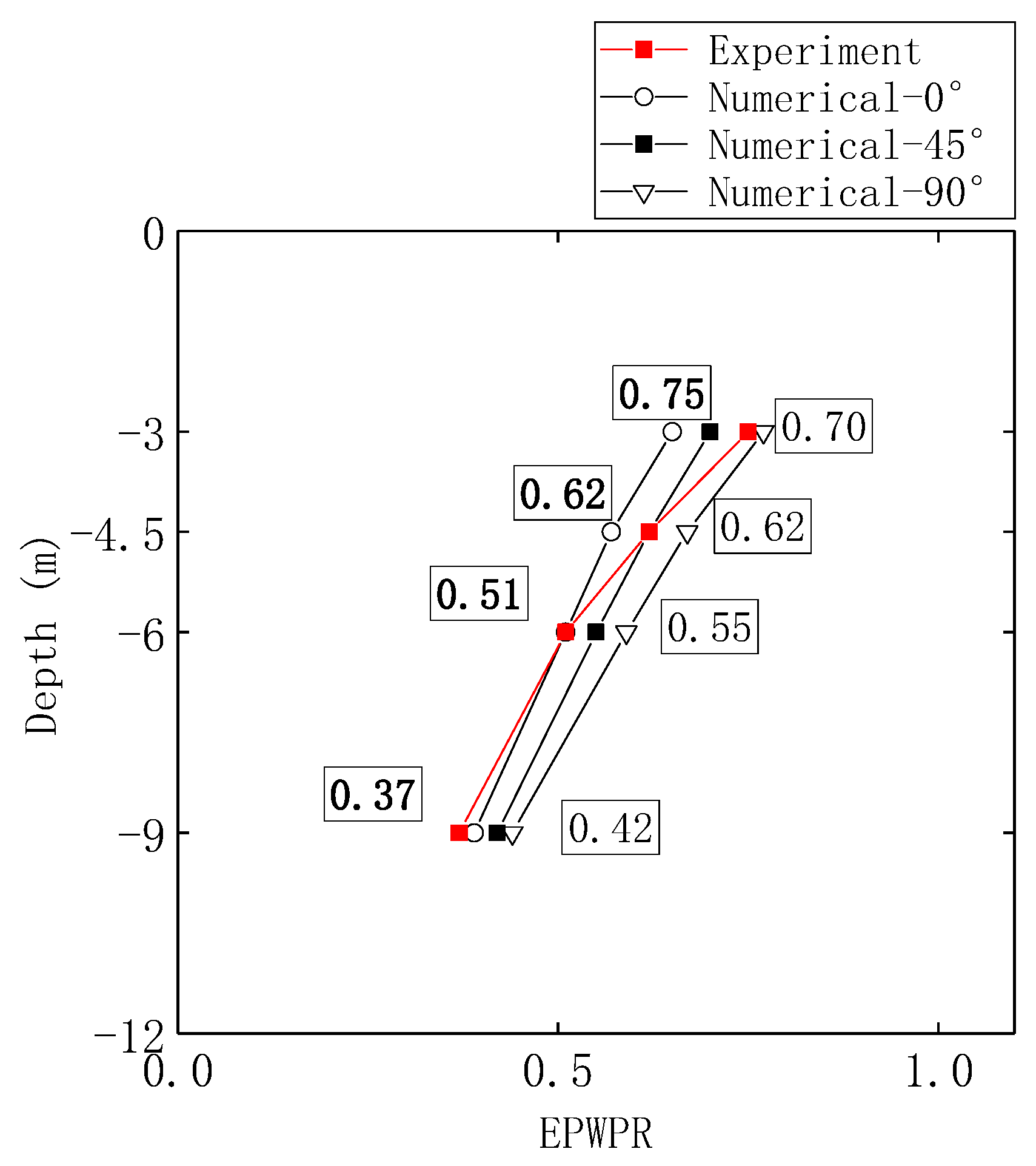
3.1.2. Excess Pore Water Pressure Ratio

The arrangement of the measuring points for the excess pore water pressure (EPWP) is shown in Figure 8. A comparison of the peak values of the excess pore water pressure ratio (EPWPR = excess pore water pressure/initial vertical effective stress) along the depth between the simulation and the test is shown in Figure 12.

Table 6. Comparison of the peak values of EPWPR at different depth.

Depth	0°	45°	90°	45° (Test)
−3.0 m	0.65	0.70	0.77	0.75
−4.5 m	0.57	0.62	0.67	0.62
−6.0 m	0.51	0.55	0.59	0.51
−9.0 m	0.39	0.42	0.44	0.37

lists the calculated peak values of the EPWPRs for various azimuth angle directions at different depths. The simulation EPWPRs at the depths of −7.5 m, −6 m, −4.5 m and −3.0 m in the 45° azimuth angle are 0.42, 0.55, 0.62, and 0.70, respectively, while the tested EPWPRs at the corresponding positions are 0.37, 0.51, 0.62, and 0.75, respectively. The results were relatively similar, but there were certain differences. the reason is mainly considered to be the change of soil permeability. The coefficient of permeability changes when soil liquefied in CST test, while the coefficient of permeability in numerical simulation is a constant value. Moreover, pore water pressure at different azimuth angles with the same distance around the pile show different response. This is obviously due to the direction of dynamic wave, indicating that anisotropy of seismic waves needs to be considered in earthquakes. In general, the simulation reflects the change in the excess pore water pressure, and the values of EPWPR with depth are consistent with the test results.

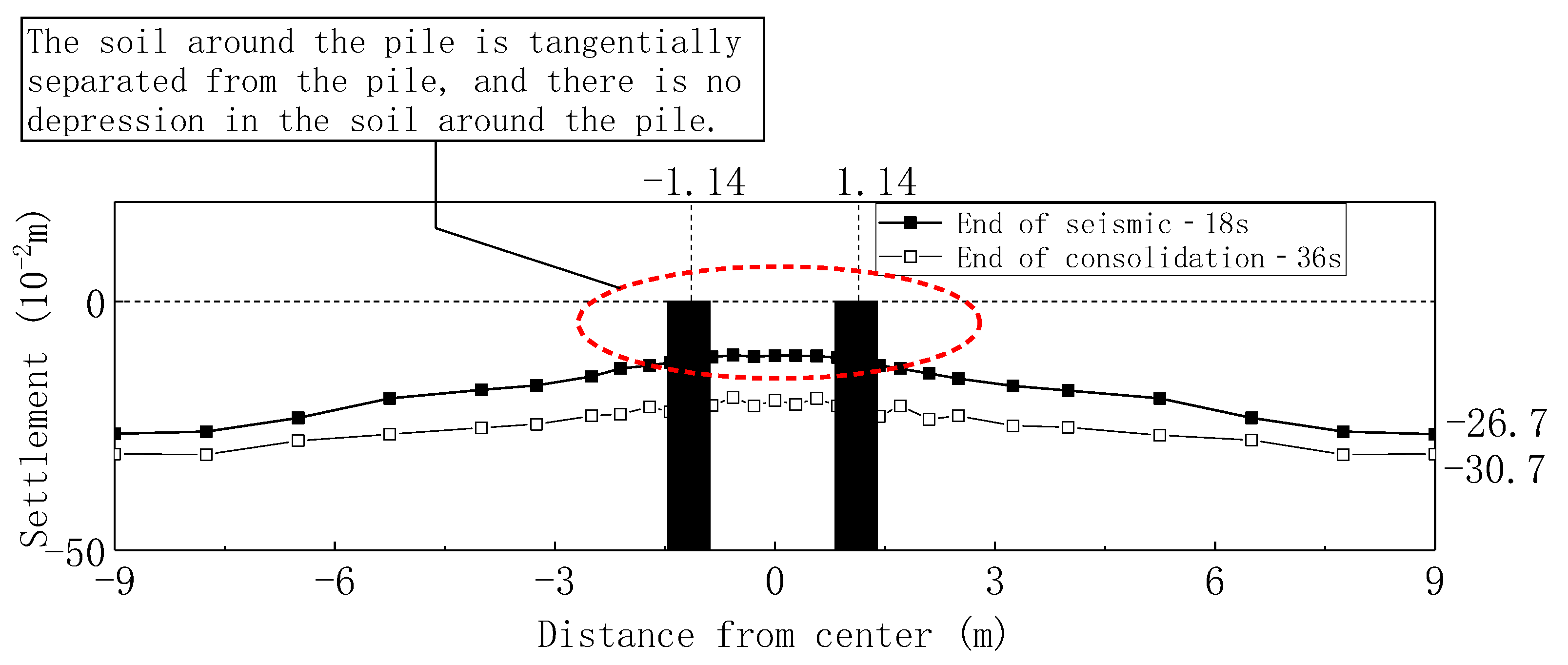
3.2. Surface Settlement

Figure 13 shows the time history of the soil surface settlement measured in the middle, near the piles. The values of settlements at the end of the vibration (18 s) and consolidation after vibration (36 s) are 18.1 cm and 25.7 cm, respectively. The settlement at the end of the CST test was measured as 18 cm in the prototype. The simulation results are consistent with the test results, which confirms the rationality and accuracy of the FE method.

Figure 14 shows the profile of soil surface settlement. The figure clearly shows that the settlement in the far field is larger than that in the middle near the piles, which confirms that the piles have the advantage of restraining foundation settlements when subjected to dynamic loading. Since joint elements were used to simulate the pile-soil contact, the soil could slide along the tangential direction of the piles, and the phenomenon of “empty” and “sag” around the piles was not obvious in the simulation results.

3.3. Pile Bending Moment

Pile 1 (see Figure 1) was selected for analysis in this section. A comparison of the pile bending moments between the simulation and test results is shown in Figure 15. The bending moment of the pile in the simulation has three peak values at the top, upper, and lower parts of the pile, which are called the first, second, and third extreme values of bending moments, respectively, for the convenience of analysis. Although the inflection points of the bending moment curve were consistent, there were certain differences in the magnitude and location of the extreme values of the bending moments. For the test results, the three peak values of bending moment envelope from shallow to deep appear at 0 m, −3.75 m and −6.30 m with corresponding values of 139.1 kN∙m, 27.5 kN∙m and 76.4 kN∙m respectively; for the simulation results, the three peak values of bending moment envelope appear at 0.275 m, −2.625 m and −5.625 m with the corresponding values of 105.6 kN∙m, 56.1 kN∙m and 90.2 kN∙m, respectively. For the result of bending moment, a difference in value between simulation and tests results was observed. The main reason might be the length of piles. Due to the limitation of centrifuge model tests, the piles in this study was not long enough. Usually, the design of pile length could be longer to penetrate the liquefiable layers, which depends on the complexity of the real ground. Therefore, the actual pile deflection in liquefied soil is more like a long pile response which is different from what was presented in this study.

As shown in Figure 16a, the first bending moment extreme value is 105.6 kN∙m, at 0.275 m (close to the soil surface); the second bending moment extreme value is 56.1 kN∙m, at −2.625 m; the third bending moment extreme value is 90.2 kN∙m at −5.625 m. Figure 16b shows the bending moment of the pile at 8.26 s when the inflection point appears at −4.125 m, and the maximum negative bending moment is 39 kN∙m at −6.375 m; Figure 16c shows the pile bending moment when the second bending moment extreme point at 8.16 s. The value of bending moment is 56.1 kN∙m at −2.625 m, but the maximum bending moment value is 62.5 kN∙m at −4.125 m, the pile has no inflection point. Figure 16d shows the pile bending moment when the third bending moment extreme value occurs at 8.68 s and the inflection point is observed at a depth of −1.40 m. The bending moment at the pile top is reversed with a value of −46.2 kN∙m.

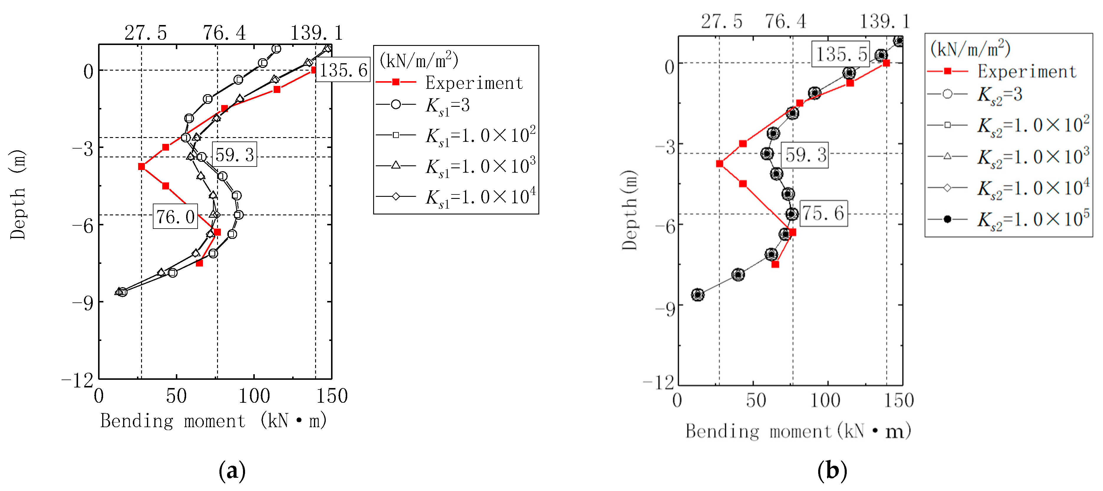
3.4. Parametric Study of Interface Elements

According to the reference parameters of joint elements [27], the normal stiffness k_n, which has little influence on the distribution of pile bending moment, is kept unchanged, and the tangential stiffness k_s on the bending moment of the pile is studied. The parameter on the surrounding side of piles is indicated as K_s1 while it was indicated as K_s2 at the pile tip. Keep K_s2 equal to 1.0 × 10² kN/m/m², and change the value of K_s1. For the bending moment of Pile 1, as shown in Figure 17a, when K_s1 increases from 3 kN/m/m² to 1 × 10⁴ kN/m/m², the first extreme value of bending moment increases to 135.6 kN∙m, at 0.275 m; the second extreme value of bending moment increases to 59.3 kN·m, and the position of occurrence moves down from −2.875 m to −3.375 m; the third extreme value of bending moment decreases to 76.0 kN·m, and the position remains unchanged at −5.625 m. Therefore, set 1.0 × 10⁴ kN/m/m² as the value of the tangential stiffness K_s1 at the pile side, and the influence of the tangential stiffness K_s2 at the pile tip on the bending moment is analyzed. As shown in Figure 17b, K_s2 has almost no effect on the bending moment of the pile, so keep K_s2 constant in a value of 1 × 10² kN/m/m². The bending moment of the pile in the numerical simulation is close to the experimental value, the tangential stiffness that K_s1 = 1.0 × 10⁴ kN/m/m² and K_s2 = 1 × 10² kN/m/m² was used in the analysis.

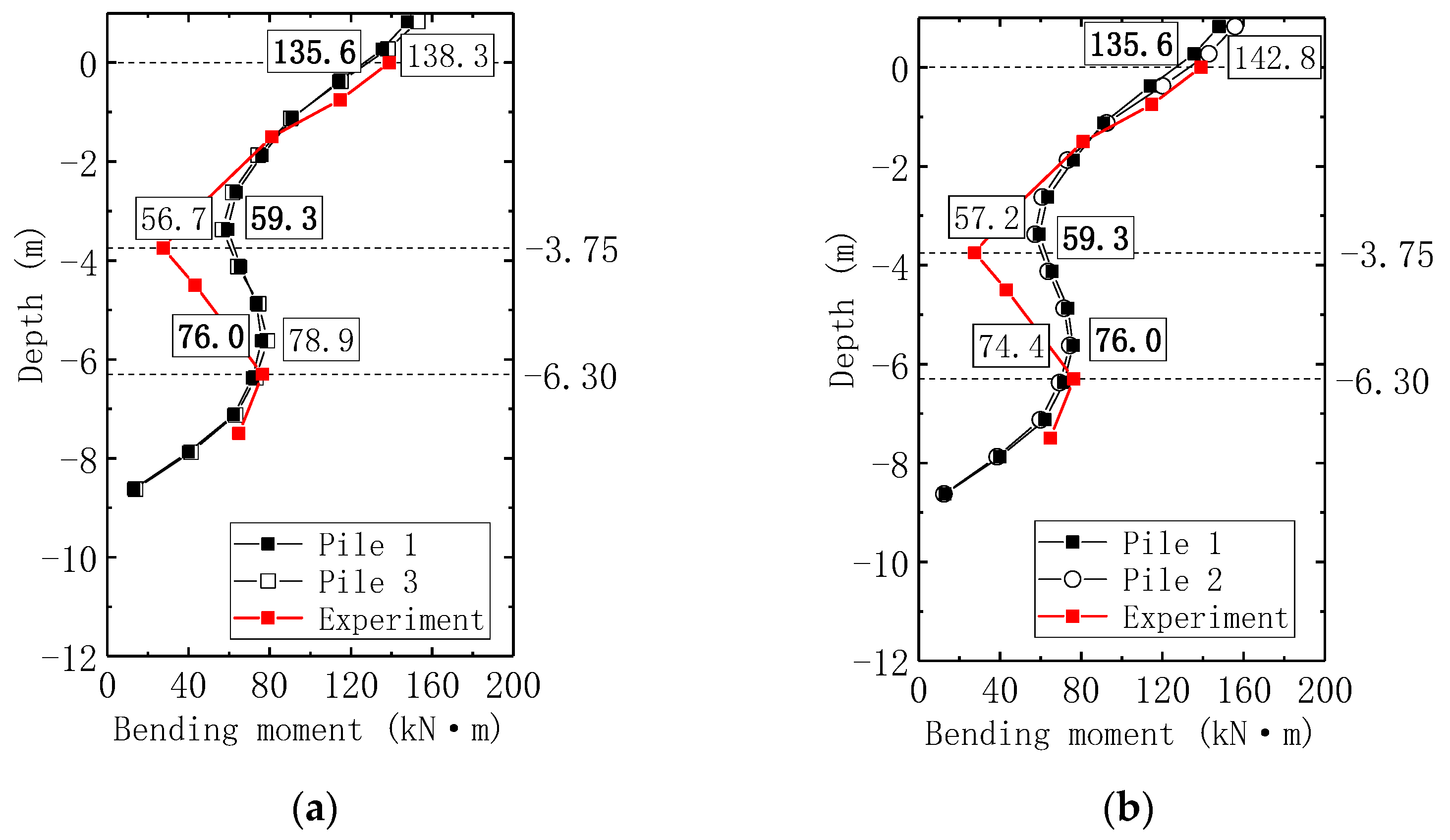
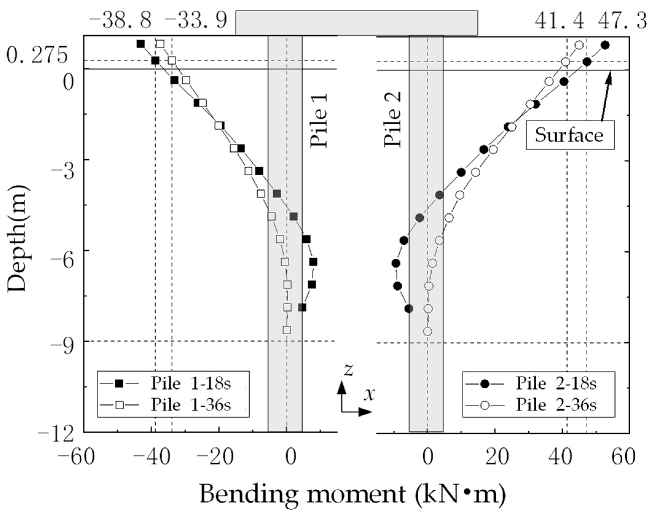
3.5. Comparison of Different Piles

Figure 18 shows arrangement of the four-pile group. Along the vibration direction (x direction), Pile 1 and Pile 3 belong to the relationship of side-by-side piles, while Pile 1 and Pile 2 belong to the relationship of front and rear piles. In Figure 19, the bending moment envelopes of Pile 1 and Pile 3, Pile 1 and Pile 2 are very close, but a small difference was observed, especially between Pile 1 and Pile 2. Furthermore, the time history curve of pile bending moment at 0.275 m close to the soil surface was selected and shown in Figure 20. The time history curves of bending moment of Pile 1 and Pile 3 are almost coincident, indicating that the motion state of the side-by-side piles in the pile group is the same. At the end of the vibration, Pile 1 and Pile 3 have almost the same residual bending moment of about −38.8 kN∙m, indicating that residual deformation or stress of the structure after dynamic loading may influence bearing capacity. The complete agreement of the bending moment curves also indicates that the residual deformation direction of the side-by-side piles is also the same. In Figure 20b, the time history curves of the bending moment of Pile 1 and Pile 2 are approximately symmetrical along the zero axis, and the value of residual bending moment is positive for Pile 2 and negative for Pile 1. The group effect for the front and rear piles indicates that the movement of the pile would be different for different pile locations and therefore the pile would behave differently under dynamic loading.

As shown in Figure 21, at the end of the vibration (18 s), the residual bending moments of Pile 1 and Pile 2 at 0.275 m are −38.8 kN∙m and 47.3 kN∙m, respectively, and there is an inflection point near −4.75 m. When the consolidation of liquefied soil is completed (36 s), the inflection point disappears, and the residual bending moments at the top of Pile 1 and Pile 2 decrease to −33.9 kN∙m and 41.4 kN∙m, respectively, which are 25% and 30% of the maximum bending moment of the pile top during vibration. This indicates that, although the pile deformation is released to a certain extent, the residual bending moment at the pile top is reduced to a limited extent compared with the bending moment at the end of the vibration. The permanent deformation of the ground soil caused deformation and a residual bending moment of the pile. Figure 22 shows the horizontal displacements of Pile 1 and Pile 2 at the end of the vibration and consolidation after vibration. The lower parts of Pile 1 and Pile 2 were squeezed inward during and after the vibration, which led to a bending moment on the outside of the pile top, as shown in Figure 21. This pile displacement can be confirmed by soil deformation, as shown in Figure 23. At the end of the vibration (18 s), the foundation soil outside the lower part of the pile tends to deform toward the pile. This ground deformation tendency leads to a residual bending moment and deformation of the pile.

4. Conclusions

In this study, the water-soil fully coupled dynamic FE method was used to perform a numerical simulation on a four-pile group foundation in saturated sand. The column element was used to consider the volume effect of the pile, and the joint element was used to consider the pile-soil contact. The dynamic responses of pile-soil interactions, such as soil acceleration, EPWPR, soil deformation, and pile bending moment, are presented in detail. The results of the numerical simulation were compared with those of the CST test, and the dynamic behaviours of the pile and soil were examined. The following conclusions were drawn.

• The accumulation of excess pore water pressure influences the stiffness of the soil, and the acceleration amplitude of shallow soil is significantly reduced. Before the soil was completely liquefied, the acceleration of the soil near the soil surface increased slightly. When the EPWPR was close to 1.0, and the soil liquefied, the dynamic acceleration was significantly attenuated, and the liquefied soil layer blocked the transmission of waves in the soil.
• The development of EPWP in the soil at different azimuth angles around the pile was different. The EPWPR of the soil at the same vibration plane as the pile (azimuth angle 0°) was the smallest, whereas the largest EPWPR appeared at the vertical vibration plane with an azimuth angle of 90°.
• Considering the volume effect of the pile through the column element, the numerical simulation was closer to the test results, and when the joint element was used in the numerical simulation of the multi-pile foundation to consider the pile-soil contact, the normal stiffness coefficient of the joint element on the side of the pile was the key to the appearance of the inverted point of the pile. Extreme values appeared on the pile top and middle or lower part of the pile. The pile exhibited evident reverse bending characteristics during vibration. This difference in the bending moment of piles at different positions in the pile group can provide an effective theoretical basis for the design of the pile group, particularly the determination of the pile group coefficient commonly used in the design code.
• The water-soil fully coupled dynamic FE-FD method can more accurately reproduce the pore water pressure distribution and reflect the change in soil acceleration with depth. Using column elements to consider the pile volume effect and the joint element to consider the pile-soil contact, the numerical method can simulate the internal force of the pile in liquefiable soil and provide an available reference for the investigation of soil-structure interaction problems.

References

1. Kandasamy, R.; Cui, F.; Townsend, N.; Foo, C.C.; Guo, J.; Shenoi, A.; Xiong, Y. A review of vibration control methods for marine offshore structures. Ocean Eng. 2016, 127, 279–297. [Google Scholar] [CrossRef]
2. Chen, W.; Du, X.; Zhang, B.-L.; Cai, Z.; Zheng, Z. Near-Optimal Control for Offshore Structures with Nonlinear Energy Sink Mechanisms. J. Mar. Sci. Eng. 2022, 10, 817. [Google Scholar] [CrossRef]
3. Lee, C.J.; Bolton, M.D.; Al-Tabbaa, A. Numerical modelling of group effects on the distribution of dragloads in pile foundations. Geotechnique 2002, 52, 325–335. [Google Scholar] [CrossRef]
4. Maeso, O.; Aznárez, J.J.; García, F. Dynamic impedances of piles and groups of piles in saturated soils. Comput. Struct. 2005, 83, 769–782. [Google Scholar] [CrossRef]
5. Tamura, S.; Ohno, Y.; Shibata, K.; Funahara, H.; Nagao, T.; Kawamata, Y. E-Defense shaking test and pushover analyses for lateral pile behavior in a group considering soil deformation in vicinity of piles. Soil Dyn. Earthq. Eng. 2021, 142, 106529. [Google Scholar] [CrossRef]
6. Hussien, M.N.; Tobita, T.; Iai, S.; Karray, M. Soil-pile-structure kinematic and inertial interaction observed in geotechnical centrifuge experiments. Soil Dyn. Earthq. Eng. 2016, 89, 75–84. [Google Scholar] [CrossRef]
7. Zhang, F.; Kimura, M. Numerical Prediction of the Dynamic Behaviors of an RC Group-Pile Foundation. Soils Found. 2002, 42, 77–92. [Google Scholar] [CrossRef]
8. Shirato, M.; Nonomura, Y.; Fukui, J.; Nakatani, S. Large-Scale Shake Table Experiment and Numerical Simulation on the Nonlinear Behavior of Pile-Groups Subjected to Large-Scale Earthquakes. Soils Found. 2008, 48, 375–396. [Google Scholar] [CrossRef]
9. Maheshwari, B.K.; Watanabe, H. Nonlinear Dynamic Behavior of Pile Foundations: Effects of Separation at the Soil-Pile Interface. Soils Found. 2006, 46, 437–448. [Google Scholar] [CrossRef]
10. Bao, X.; Morikawa, Y.; Kondo, Y.; Nakamura, K.; Zhang, F. Shaking table test on reinforcement effect of partial ground improvement for group-pile foundation and its numericalsimulation. Soils Found. 2012, 52, 1043–1061. [Google Scholar] [CrossRef]
11. Shi, L.; Xu, C.; Cai, Y.; Geng, X. Dynamic impedances and free-field vibration analysis of pile groups in saturated ground. J. Sound Vib. 2014, 333, 3709–3731. [Google Scholar] [CrossRef]
12. Ebeido, A.; Elgamal, A.; Tokimatsu, K.; Abe, A. Pile and Pile-Group Response to Liquefaction-Induced Lateral Spreading in Four Large-Scale Shake-Table Experiments. J. Geotech. Geoenviron. Eng. 2019, 145, 04019080. [Google Scholar] [CrossRef]
13. Xu, C.; Dou, P.; Du, X.; El Naggar, M.H.; Miyajima, M.; Chen, S. Seismic performance of pile group-structure system in liquefiable and non-liquefiable soil from large-scale shake table tests. Soil Dyn. Earthq. Eng. 2020, 138, 106299. [Google Scholar] [CrossRef]
14. Emani, P.K.; Maheshwari, B.K. Dynamic impedances of pile groups with embedded caps in homogeneous elastic soils using CIFECM. Soil Dyn. Earthq. Eng. 2009, 29, 963–973. [Google Scholar] [CrossRef]
15. Sarkar, R.; Maheshwari, B.K. Effects of Separation on the Behavior of Soil-Pile Interaction in Liquefiable Soils. Int. J. Géoméch. 2012, 12, 1–13. [Google Scholar] [CrossRef]
16. Luo, C.; Yang, X.; Zhan, C.; Jin, X.; Ding, Z. Nonlinear 3D finite element analysis of soil–pile–structure interaction system subjected to horizontal earthquake excitation. Soil Dyn. Earthq. Eng. 2016, 84, 145–156. [Google Scholar] [CrossRef]
17. Zhang, C.; Deng, P.; Ke, W. Assessing physical mechanisms related to kinematic soil-pile interaction. Soil Dyn. Earthq. Eng. 2018, 114, 22–26. [Google Scholar] [CrossRef]
18. Chatterjee, K.; Choudhury, D.; Murakami, A.; Fujisawa, K. P-y Curves of 2x2 pile group in liquefiable soil under dynamic loadings. Arab. J. Geosci. 2020, 13, 585. [Google Scholar] [CrossRef]
19. Saha, R.; Dutta, S.C.; Haldar, S.; Kumar, S. Effect of soil-pile raft-structure interaction on elastic and inelastic seismic behavior. Structures 2020, 26, 378–395. [Google Scholar] [CrossRef]
20. Rahmani, A.; Pak, A. Dynamic behavior of pile foundations under cyclic loading in liquefiable soils. Comput. Geotech. 2012, 40, 114–126. [Google Scholar] [CrossRef]
21. Motamed, R.; Towhata, I.; Honda, T.; Tabata, K.; Abe, A. Pile group response to liquefaction-induced lateral spreading: E-Defense large shake table test. Soil Dyn. Earthq. Eng. 2013, 51, 35–46. [Google Scholar] [CrossRef]
22. Hussein, A.F.; El Naggar, M.H. Seismic axial behaviour of pile groups in non-liquefiable and liquefiable soils. Soil Dyn. Earthq. Eng. 2021, 149, 106853. [Google Scholar] [CrossRef]
23. Xiong, Y.; Bao, Y.; Ye, B.; Ye, G.; Zhang, F. 3D dynamic analysis of the soil–foundation–superstructure system considering the elastoplastic finite deformation of both the soil and the superstructure. Bull. Earthq. Eng. 2018, 16, 1909–1939. [Google Scholar] [CrossRef]
24. Castro, G.; Poulos, S.J. Factors affecting liquefaction and cyclic mobility. J. Geotech. Eng. Div. -Asce 1980, 106, 211–214. [Google Scholar] [CrossRef]
25. Knappett, J.A.; Madabhushi, S.P. Liquefaction-Induced Settlement of Pile Groups in Liquefiable and Laterally Spreading Soils. J. Geotech. Geoenviron. Eng. 2008, 134, 1609–1618. [Google Scholar] [CrossRef]
26. Bao, X.; Ye, G.; Ye, B.; Fu, Y.; Su, D. Co-seismic and post-seismic behavior of an existed shallow foundation and super structure system on a natural sand/silt layered ground. Eng. Comput. 2016, 33, 288–304. [Google Scholar] [CrossRef]
27. Bao, X.; Wu, S.; Liu, Z.; Su, D.; Chen, X. Study on the nonlinear behavior of soil–pile interaction in liquefiable soil using 3D numerical method. Ocean Eng. 2022, 258, 111807. [Google Scholar] [CrossRef]
28. Zhang, F.; Ye, B.; Noda, T.; Nakano, M.; Nakai, K. Explanation of Cyclic Mobility of Soils: Approach by Stress-Induced Anisotropy. Soils Found. 2007, 47, 635–648. [Google Scholar] [CrossRef]
29. Ye, B.; Ye, G.; Zhang, F.; Yashima, A. Experiment and Numerical Simulation of Repeated Liquefaction-Consolidation of Sand. Soils Found. 2007, 47, 547–558. [Google Scholar] [CrossRef]
30. Ye, B.; Hu, H.; Bao, X.; Lu, P. Reliquefaction behavior of sand and its mesoscopic mechanism. Soil Dyn. Earthq. Eng. 2018, 114, 12–21. [Google Scholar] [CrossRef]
31. Ye, G. DBLEAVES: User’s Manual [DB/CD]; Shanghai Jiaotong University: Shanghai, China, 2013. [Google Scholar]
32. Ye, B.; Ye, G.; Zhang, F. Numerical modeling of changes in anisotropy during liquefaction using a generalized constitutive model. Comput. Geotech. 2012, 42, 62–72. [Google Scholar] [CrossRef]
33. Arulanandan, K.; Sybico, J. Post-liquefaction settlement of sand mechanism and in situ evaluation. In Proceedings of the Fourth Japan–US Workshop on Earthquake Resistant Design of Lifeline Facilities and Countermeasures for Soil Liquefaction, Honolulu, HI, USA, 27–29 May 1992. [Google Scholar]
34. Shahir, H.; Pak, A.; Taiebat, M.; Jeremić, B. Evaluation of variation of permeability in liquefiable soil under earthquake loading. Comput. Geotech. 2012, 40, 74–88. [Google Scholar] [CrossRef]
35. Su, D. Centrifuge Investigation on Responses of Sand Deposit and Sand-Pile System under Multi-Directional Earthquake Loading; The Hong Kong University of Science and Technology: Hong Kong, China, 2005. [Google Scholar]
Figure 1. Finite element model of soil-pile group-superstructure system.
Jmse 10 01026 g001
Figure 2. Sectional view of laminar box and model piles with data acquisition equipment (PPTn: pore presur test number; ACC: acceleration).
Jmse 10 01026 g002
Figure 3. Time history of input dynamic wave.
Jmse 10 01026 g003
Figure 4. Model of pile composed of beam element and column element.
Jmse 10 01026 g004
Figure 5. Schematic diagram of the joint element.
Jmse 10 01026 g005
Figure 6. Relationship between stress and strain for the joint element: (a) σt-u; (b) τ-w.
Jmse 10 01026 g006
Figure 7. Observation points of acceleration in soil and pile top.
Jmse 10 01026 g007
Figure 8. Observation points of excess pore water pressure in soil.
Jmse 10 01026 g008
Figure 9. Distribution of initial effective stress in vertical direction in the ground.
Jmse 10 01026 g009
Figure 10. Time history of acceleration in the ground (90°): (a) At the position of superstructure; (b) At the position of 0.0 m; (c) At the position of −3 m; (d) At the position of −7.5 m; (e) At the position of −12 m.
Jmse 10 01026 g010
Figure 11. Numerical simulation and test results of peak acceleration at different depth in soil.
Jmse 10 01026 g011
Figure 12. Numerical simulation and test results of peak value of EPWPR.
Jmse 10 01026 g012
Figure 13. Time history of soil surface settlement.
Jmse 10 01026 g013
Figure 14. Simulation settlement profile at ground surface.
Jmse 10 01026 g014
Figure 15. Numerical simulation and test results of bending moment envelope of pile.
Jmse 10 01026 g015
Figure 16. Bending moment and extreme values of Pile 1 at different times: (a) Bending moment envelope; (b) Bending moment at 8.26 s; (c) Bending moment at 8.16 s; (d) Bending moment at 8.68 s.
Jmse 10 01026 g016
Figure 17. Influence of tangential stiffness on bending moment of Pile 1: (a) Change the value of tangential stiffness Ks1; (b) Change the value of tangential stiffness Ks2.
Jmse 10 01026 g017
Figure 18. Arrangement of four-pile group.
Jmse 10 01026 g018
Figure 19. Bending moment envelopes of different piles: (a) Pile 1 and Pile 3; (b) Pile 1 and Pile 2.
Jmse 10 01026 g019
Figure 20. Time history of bending moments at 0.275 m of different piles: (a) Pile 1 and Pile 3; (b) Pile 1 and Pile 2.
Jmse 10 01026 g020
Figure 21. Bending moment of Pile 1 and Pile 2 at 18 s and 36 s.
Jmse 10 01026 g021
Figure 22. Horizontal displacement of Pile 1 and Pile 2 at 18 s and 36 s.
Jmse 10 01026 g022
Figure 23. Displacement vector at the end of dynamic loading (deformation being amplified 10 times).
Jmse 10 01026 g023