Modeling and Dynamic Analysis of a Triple-Tagline Anti-Swing System for Marine Cranes in an Offshore Environment

Abstract

Payload lifting is inefficient and high-risk under rough sea conditions. Thus, it is not easy to achieve precise assembly, and the swing payload is liable to collide with other structures on deck and cause damage. In this paper, to explore the complex dynamic characteristics of a triple-tagline anti-swing system (TTAS) for marine cranes in an offshore environment, an irregular wave model was first integrated into a dynamic system model of TTAS, and the TTAS for offshore payload lifting was simplified as a constrained-pendulum system with moving base excitations. Further, the dynamic system model was established by applying the methods in robotics. Meanwhile, the dynamic characteristics were simulated and analyzed using Matlab/Simulink. The simulation results show that the in-plane angle and out-of-plane angle of the payload can be effectively suppressed, and the range of the two-dimensional trajectory of the payload is greatly reduced. The research results provide a theoretical basis for optimizing the mechanical structures of TTAS or similar equipment.

1. Introduction

As one of the most significant pieces of deck equipment, the ship crane is a necessary piece of mechanical equipment for cargo handling, pipe installation, replenishment, etc. Due to the unique working environment, marine cranes have more complex external excitation than onshore cranes. Due to offshore environment loads such as wind, waves, flow, and surge, a ship’s six-degree-of-freedom movement is induced persistently, resulting in significant payload swing during lifting operations. This reduces the operational efficiency of the crane but also threatens the operators’ safety. Therefore, the swing control of marine cranes is of great significance for the protection and efficiency of crane operations.

Over the past several decades, the study and design of anti-swing control strategies for cranes have greatly interested researchers. Smoczek [1] proposed a swing control technique based on the fuzzy logic and pole configuration methods, and a crane workspace identification method based on a stereo vision system. Chang [2] used a specific mechanical structure to consume the payload’s swinging energy by reducing the payload’s kinetic energy or increasing the crane system’s rigidity. Mc [3] introduced a controller design method considering the variation in wire-rope length. Andres [4] proposed a control technique to prevent payload swing, which can quickly locate the moving payload. Tran [5] established a ship-to-shore container crane model through sensitivity analysis of the input parameters of the structural response. Maghsoudi [6] proposed an improved single-degree-of-freedom swing control scheme, which can effectively adapt to the dynamic change in wire-rope length. However, due to the complexity of the offshore environment, the anti-swing control method developed based on land-based cranes cannot be directly applied to marine cranes.

Regarding research on the anti-swing technology of marine cranes, researchers worldwide have made some achievements in dynamic analysis and control algorithms. In 1997, Guo [7] designed a mechanical anti-swing device called the Maryland Rig (Maryland Rigging), which uses friction between the pulley and ropes to suppress the payload swing. Bing [8] proposed an optimal control scheme for Maryland Rigging. A feedforward control loop to the control system, proposed by Kimiaghalam [9], and the luff angle of the boom were employed as the control output to compensate for the ship’s roll motion. Numerical simulation results showed that the control effect of payload swing could be improved from 50% to 98% by the combination of feedforward and feedback control. Van [10] proposed a mechanical control device based on energy dissipation to reduce the influence of waves on marine crane operation, and a simulation verified the proposed mechanism’s effectiveness. Yan [11] studied the dynamics of cranes and proposed modeling methods to describe their behaviors in the waves. Fragopoulos [12] proposed a generalized predictive control (GPC) method, and the simulation results showed that the control system’s performance can be improved. Ren [13] proposed a general model-free anti-swing control scheme that achieves the control effect when the model parameters are unknown without considering the state-space equation. Küchler [14,15] developed a control system to reduce the swing of payload in an offshore environment. He proposed a prediction algorithm for the linear model to suppress the payload swing through active compensation. Hong and Ngo [16] designed a sliding-mode controller for a mobile harbor crane. The simulation results showed that the proposed method has a good suppression effect on the lateral swing of the payload but a poor suppression effect on the longitudinal swing. Kharola [17] established a fuzzy controller for the swing of the crane load and analyzed the influence of load mass and the crane boom’s length on the crane’s stability. Ismail [18] studied the robust control method of the marine crane systems under bounded disturbance and high sea states. The proposed quadratic optimal method of solving the sliding surface parameters can achieve good tracking performance for the predetermined trajectory of the marine crane. Ku [19] used a PD controller to control the tagline’s tension in real-time, built a 1:100 floating crane model, and verified the payload anti-swing effect through simulation analysis and experiments. An analytical model of marine crane dynamics based on a rigid–flexible coupling virtual prototype, which provides a reference significance for the design of maritime cranes, was proposed by He [20]. Martin [21,22] considered a shipboard 5-DOF gantry and even a 6-DOF and 7-DOF knuckle boom crane, developing a sliding-mode controller and anti-swing trajectory modification system that provided anti-swing control in the deck coordinate frame tracking real-time, time-varying trajectories. The automatic control of marine cranes working under harsh sea conditions was studied by Liu [23]; using the composite signal as feedback, a nonlinear controller that can respond to the uncertainty of the crane’s swing was constructed, achieving better overall control performance and stronger robustness. Lu [24] proposed a marine crane nonlinear control strategy that can also ensure the asymptotic stability of the equilibrium point of the closed-loop system under continuous ship-swing interference. The feasibility and effectiveness of the proposed method were verified experimentally. In recent years, offshore replenishment, wind farm installation, and other operations have become more frequent, often carried out under high sea conditions. Such lifting operations are often inefficient and risky. There are few studies on the dynamics and motion compensation control of the payload under the excitation of a moving base.

The complex dynamic characteristics of TTAS in the offshore environment are deeply explored, and the contributions of this paper are reflected in three aspects:

(1) The irregular wave model is first integrated into the dynamic system model of TTAS. Based on this, the system’s dynamic characteristics are simulated and analyzed, and the tendency of the payload swing angle and the two-dimensional trajectory of the payload are explored.

(2) Under irregular environment excitation, the effect of payload swing reduction is simulated and analyzed comparatively for scenarios with or without anti-swing control. The results show that the average amplitude of the in-plane angle is reduced by 63%, and that of the out-of-plane angle is reduced by 82% by using TTAS, which verifies its fidelity in the offshore environment.

(3) It is found that under irregular environment excitation, the shape of the two-dimensional trajectory of the payload is elliptic without anti-swing control, and it is 8-shaped or triangular with anti-swing control. Compared with no anti-swing control, the two-dimensional trajectory of the payload is reduced by more than 90% with anti-swing control, which can provide a theoretical basis for the optimization of the TTAS structure in the later period.

This paper is outlined as follows. The “TTAS overall architecture” section introduces the anti-swing principle of the system. The “Structure of TTAS” section briefly introduces the structure of the TTAS. The “Dynamic modeling of TTAS” section is derived from the dynamic models of the TTAS. The “Dynamic analysis” section compares the payload swing angle’s tendency and the payload’s two-dimensional trajectory with or without TTAS control. The “conclusion” section draws the research conclusion and explains the future research work.

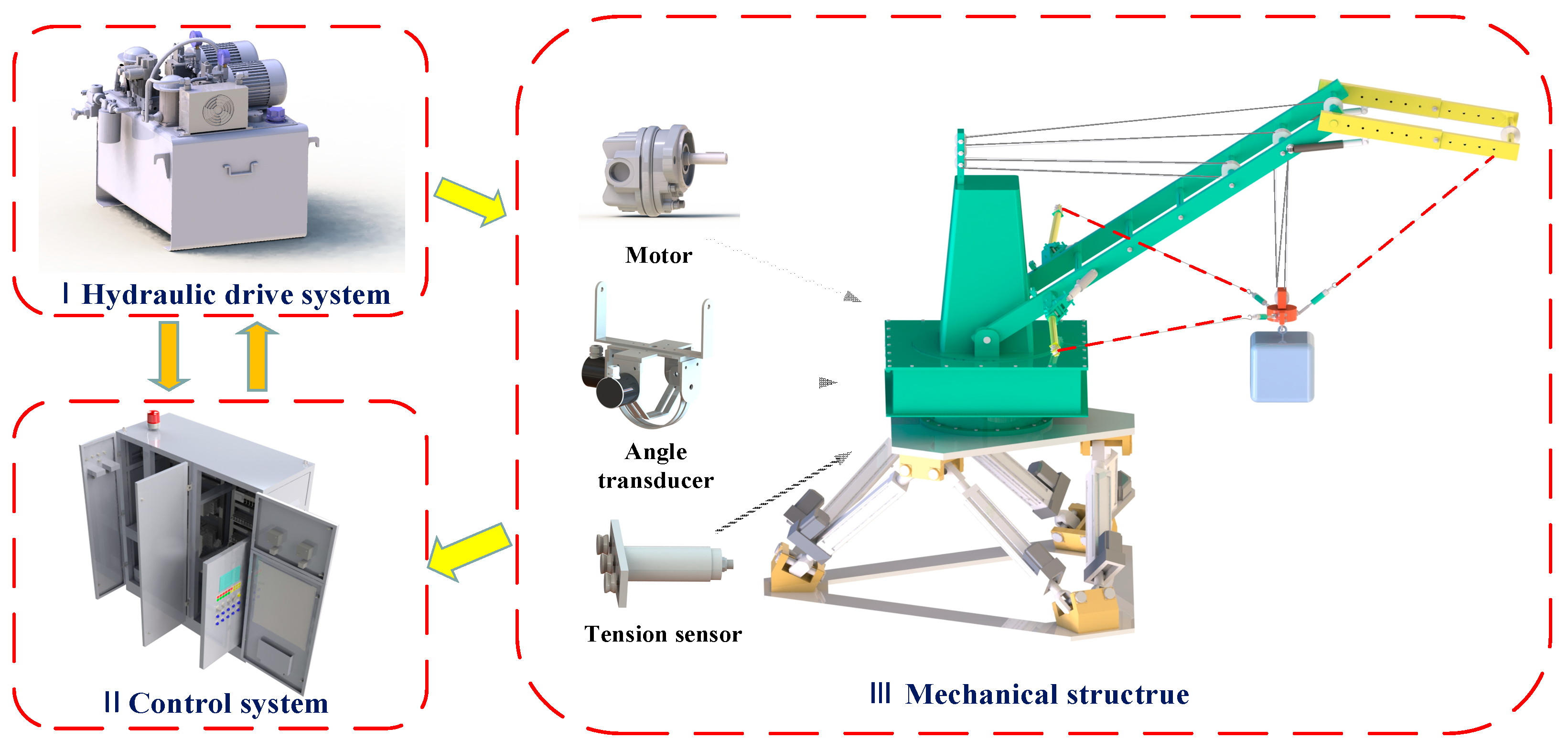
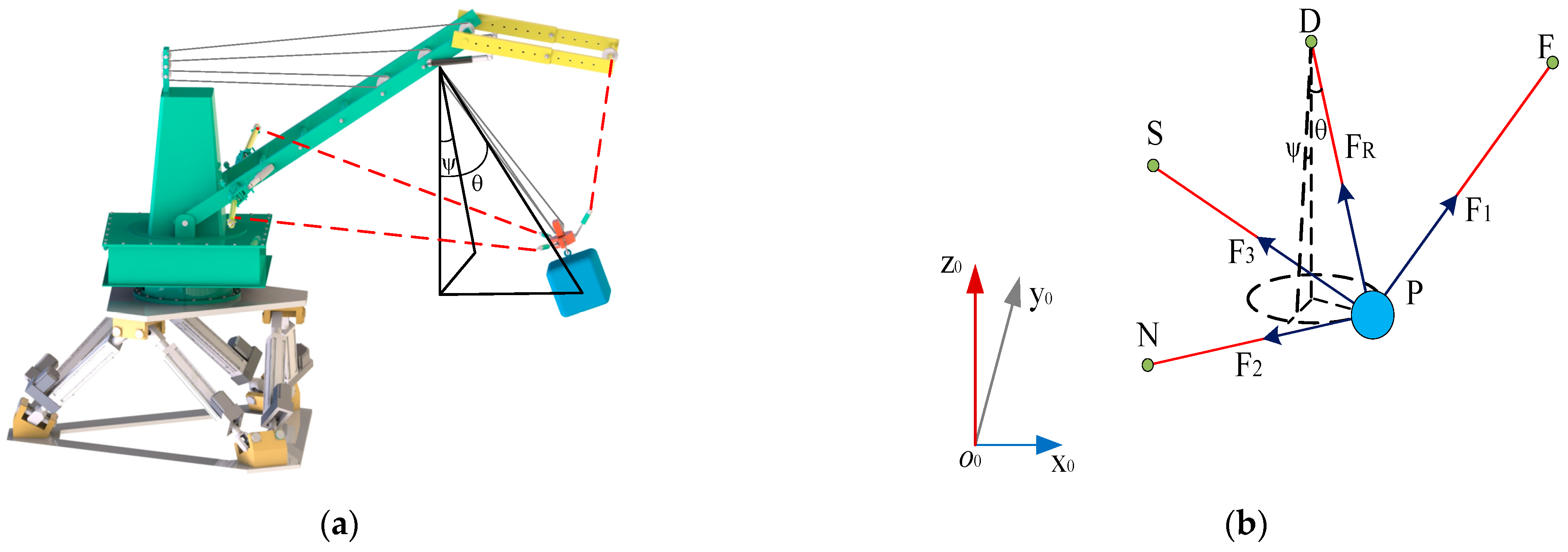
2. TTAS Overall Architecture

TTAS comprises I—a hydraulic drive system, II—a control system, and III—a mechanical structure. The mechanical design mainly includes the anti-swing knuckle jib, guide wheels, motor, tension sensor, etc., and especially realizes the fixing and guiding of the tagline position in space. At the same time, the measuring unit on the mechanical structure detects the crane action, the winch angle, the tension of the anti-swing taglines, and the swing angle of the payload. The driving system provides the power for the winch to rotate; The control system reads each sensor’s parameters and calculates the crane’s altitude and tagline-driven parallel mechanism. According to the dynamics model of the TTAS, the real-time length and tension values of the tagline are calculated. Then, the real-time control instructions of the winch are calculated using the anti-swing control measures. The main principle of TTAS is to increase three anti-swing knuckle jibs, and the ends of the anti-swing taglines merge at the hook to form a stable force triangle to achieve payload swing suppression.

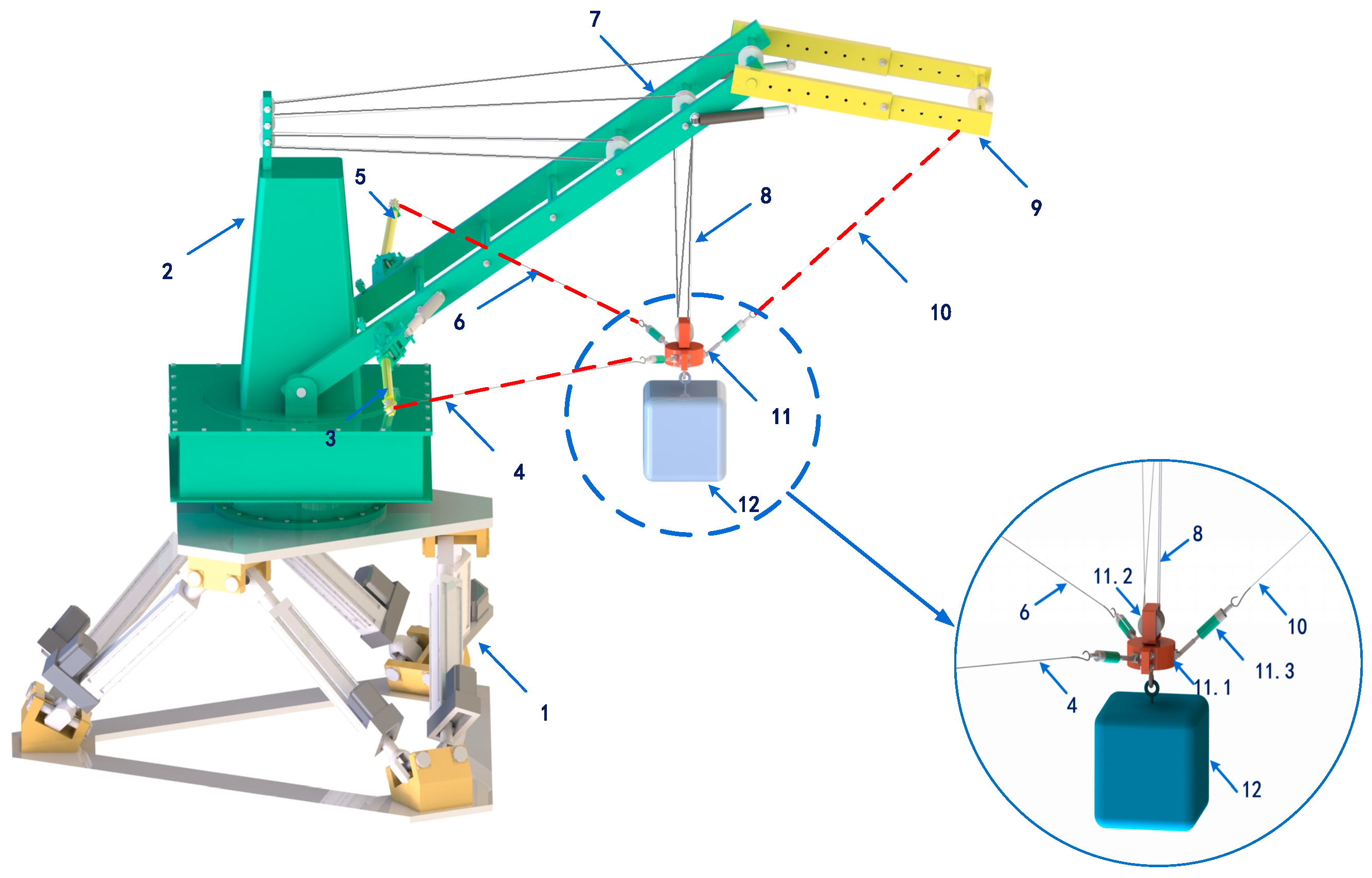
3. Structure of TTAS

Three taglines and a hoist cable must be synchronously retracted when the marine crane is luffing, lifting, or slewing to avoid disturbance to the crane itself. So, we designed a cable-driven anti-swing system for payload lifting, as shown in Figure 1. The marine crane is equipped with TTAS, and the crane comprises a hook, a hoist cable, the main jib, and the crane housing. The TTAS contains three anti-swing knuckle jibs, three anti-swing taglines, and a driving system. The TTAS can suppress the payload swing in any direction. Meanwhile, the direction of the hoist cable can be kept in a vertical or near-vertical state.

4. Dynamic Modeling of TTAS

Figure 2 shows the mechanical structure. The following assumptions are made for this system:

(1)

The jibs of marine cranes equipped with TTAS are rigid bodies.

(2)

The elastic deformation of the three taglines and the hoist cable is ignored.

(3)

The hook and payload can be considered a mass point.

(4)

The dynamic model of TTAS is established when the crane is stationary. It does not consider the crane’s own rotation and luffing.

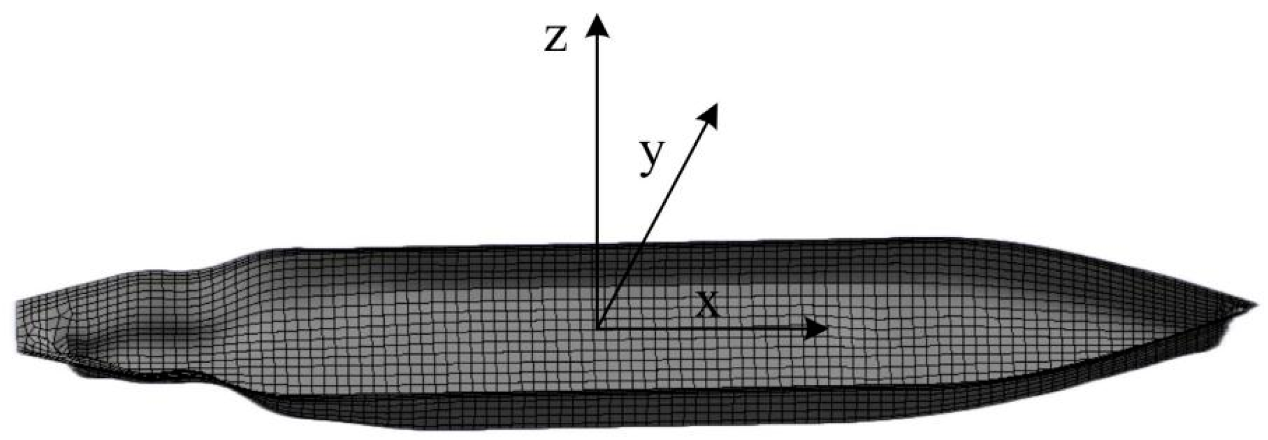
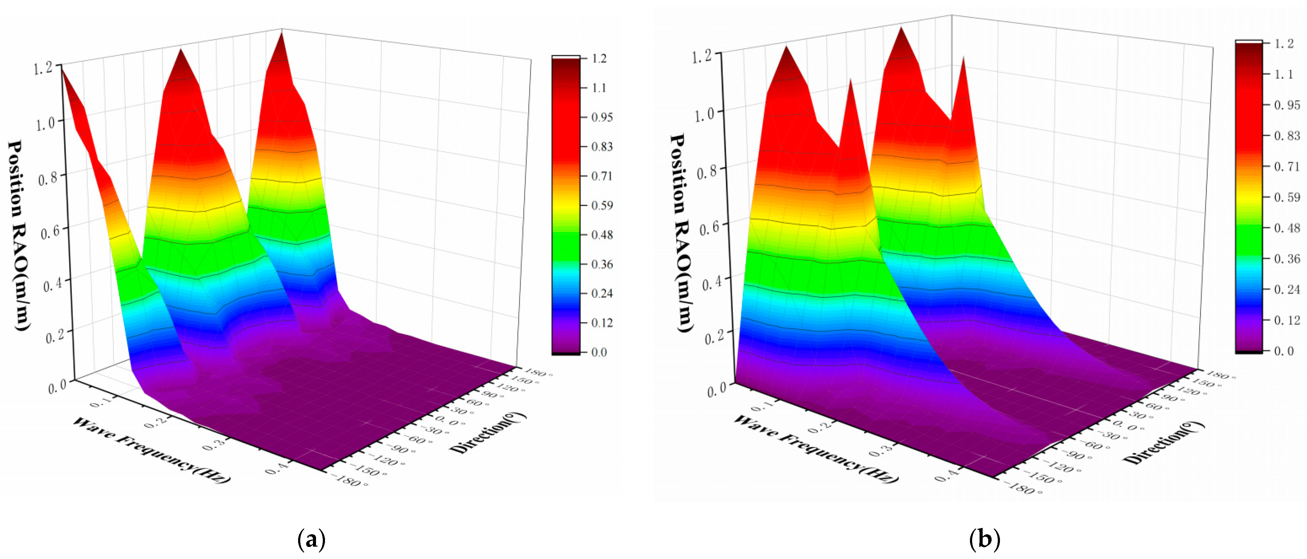
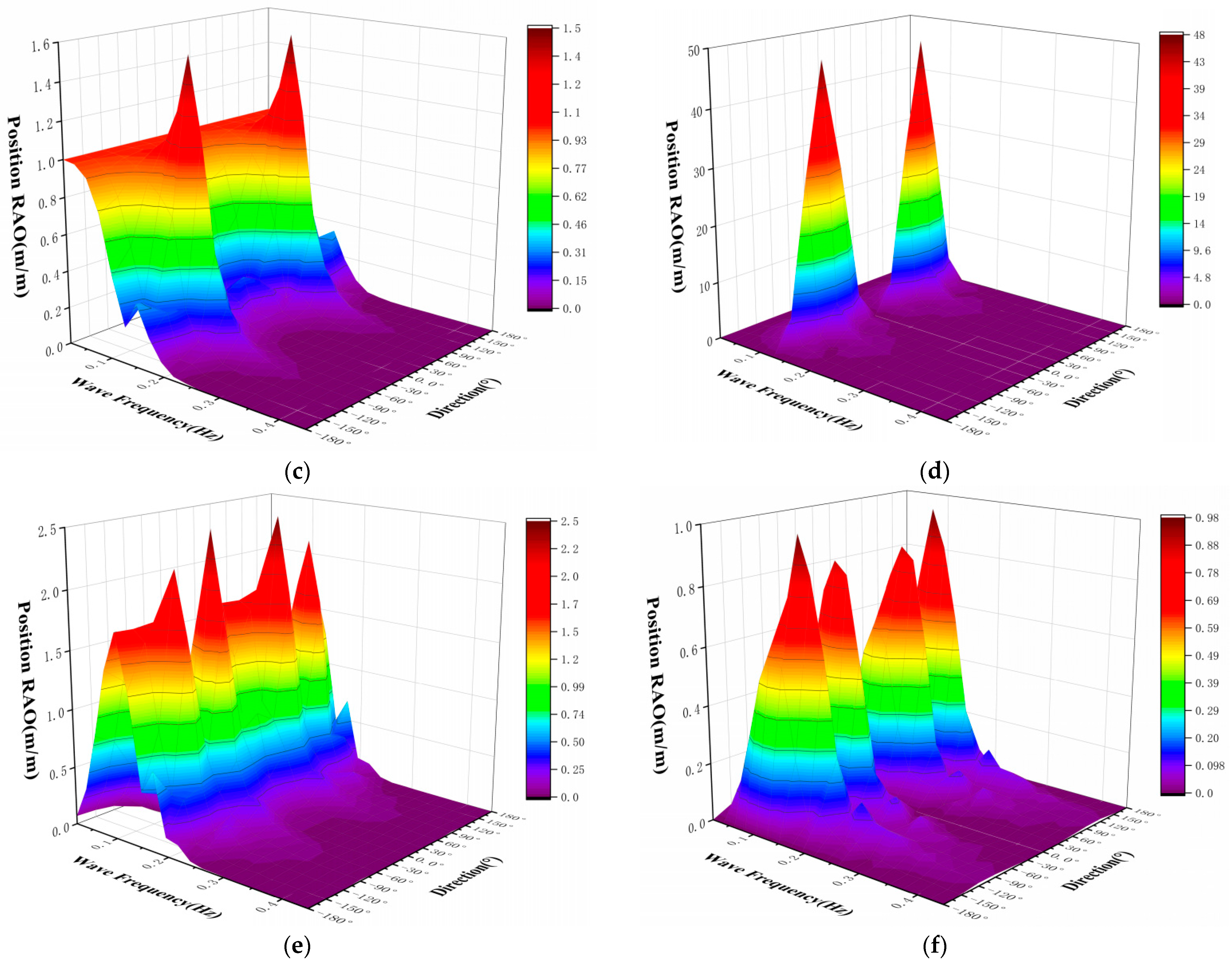
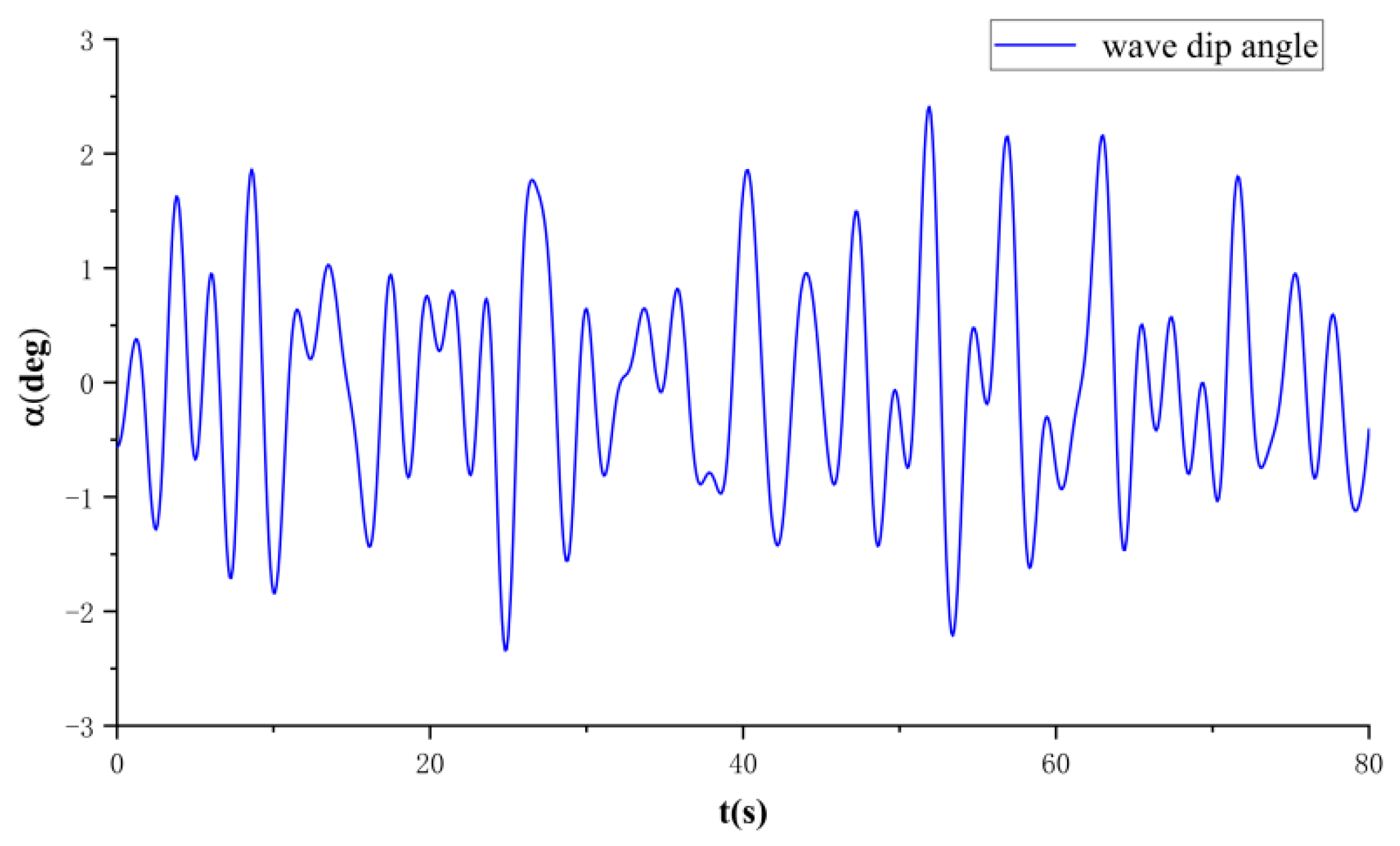
4.1. Wave-Load Model

In an ideal incompressible fluid in a irrotational field, the velocity potential satisfies the Laplace Equation and can be written as:

$${\nabla }^2\varphi =0$$

(1)

The velocity potential can be solved according to the equation:

$$\nu =\nabla \varphi$$

(2)

To obtain the speed distribution, we can use the Lagrange equation:

$$\frac{\partial \phi }{\phi t}+\frac{p}{\rho }+\frac{1}{2}{\nu }^2+gz=f(t)$$

(3)

It is assumed that the flow field of the floating body is non-rotational, non-viscous, and incompressible, the wave is a micro-wave, and the velocity potential of the flow field around the floating body is composed of three parts:

$$\varphi ={\varphi }^{-i\omega t}=\left[({\varphi }_{\mathrm{I}}+{\varphi }_{\mathrm{D}})+{\displaystyle \sum _{j=1}^6{\varphi }_j{x}_j}\right]e^{-i\omega t}$$

(4)

The wave frequency is φ for the rule; φ_I is the potential for the incident wave speed; φ_D is the potential for the diffraction wave speed; φ_j is the six degrees of freedom in the direction of the velocity potential (j = 1, 2, 3, 4, 5, 6).

The incident wave velocity potential can be expressed as:

$${\varphi }_I{e}^{-i\omega t}=-\frac{igA\cosh (k(z+h))}{\omega \cosh (kh)}{e}^{-i\left[\omega t+k(x\cos \beta +y\sin \beta )+\alpha \right]}$$

(5)

h is the depth of the water, and the incident wave amplitude is A. K is the wave number, which satisfies the dispersion relation:

$${\omega }^2=gk\tanh (kh)$$

(6)

The wave excitation force and hydrostatic pressure caused by the incident potential and diffraction potential of the floating-body structure in waves can be expressed as:

$$p=-{\rho }_{\mathrm{W}}\left(\frac{\partial {\varphi }_I}{\partial t}+\frac{\partial {\varphi }_D}{\partial t}\right)-{\rho }_{\mathrm{w}}gz$$

(7)

The wave force and moment of the floating body in the water are, respectively:

$$F_{wa}^d=-{\displaystyle \underset{S}{\iint }}(p\cdot n^d)\cdot ds$$

(8)

$$M_{wa}^d=-{\displaystyle \underset{S}{\iint }}(r\times n^d)\cdot ds$$

(9)

$F_{wa}^d$ and $M_{wa}^d$ are the wave forces on the floating body in the D-axis direction, respectively; d takes x, y and z, respectively, to represent the load components in the direction of each coordinate axis; S is the wet surface of floating body; r is the action moment arm; n^d is the component of the normal vector in the floating body pointing to the flow field in the D-axis direction.

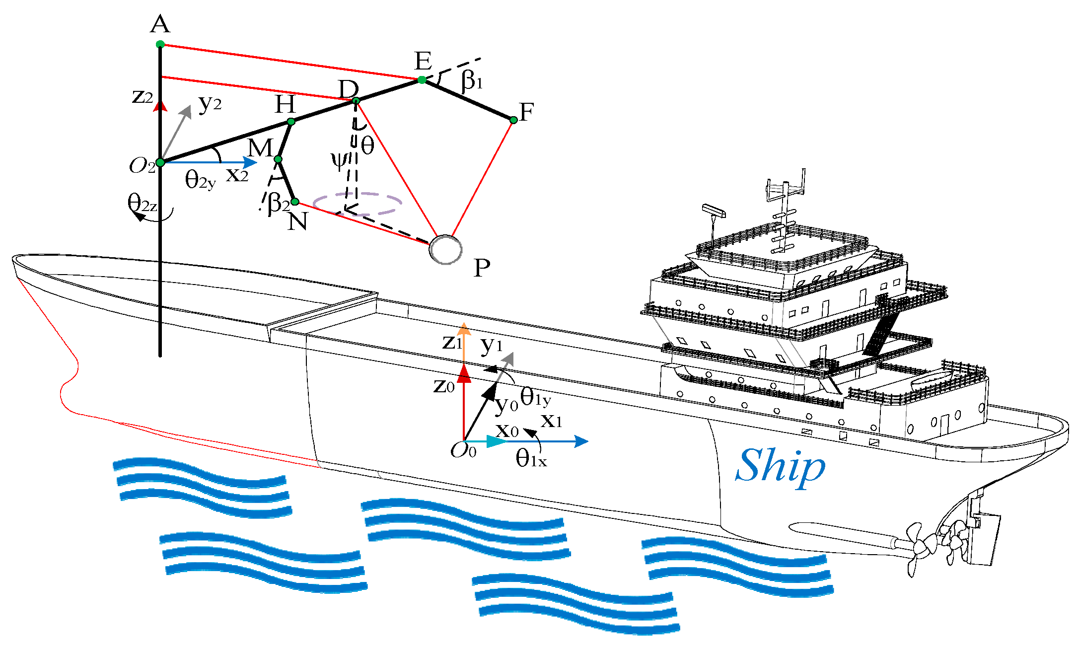
4.2. Kinematic Model

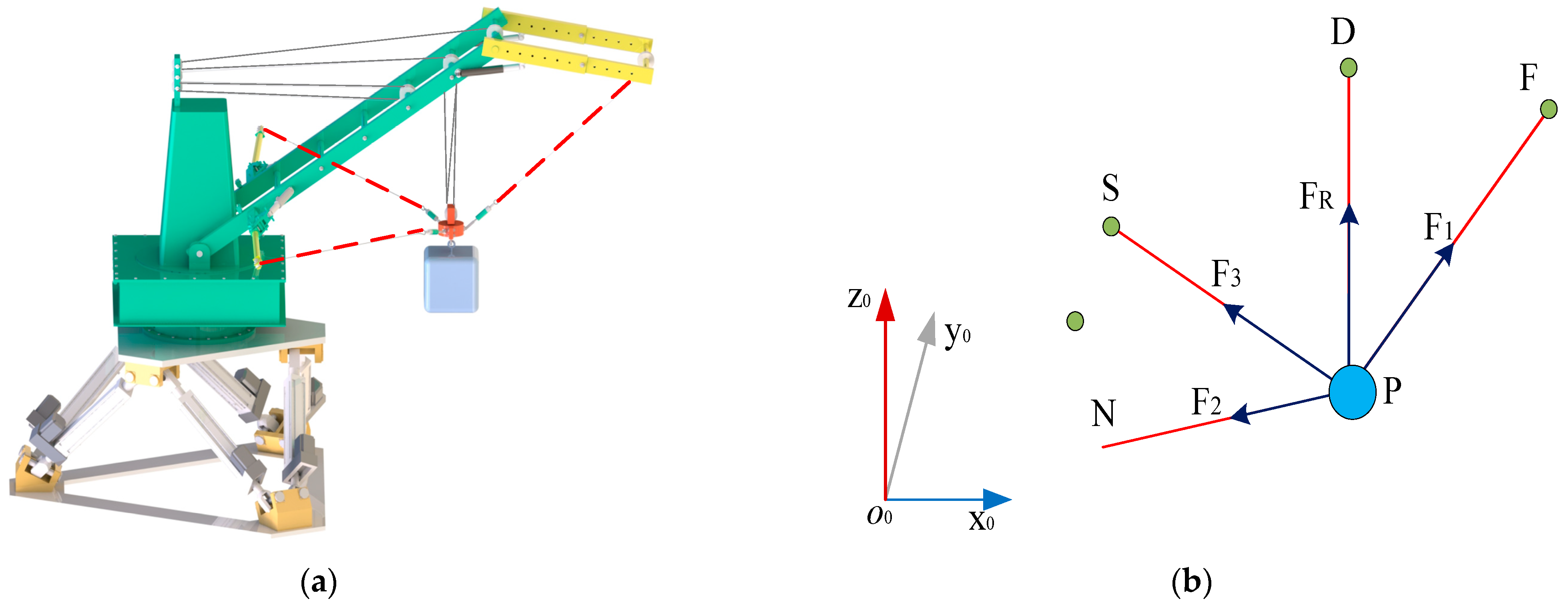
Geometrically, Figure 3 shows the simplified diagram of the marine crane with TTAS, and Figure 4 shows the top view of mechanical structure. As illustrated, x₀y₀z₀ is defined as the inertial frame, x₁y₁z₁ the ship-based frame, and x₂y₂z₂ the crane-based frame. It is assumed that the hook is close enough to the payload. The hook and the payload can be expressed as P. O₂E represents the main jib, and PD the hoist cable; EF, HMN, and HRS represent anti-swing knuckle jibs I, II, and III, respectively; and PF, PN, and PS represent taglines I, II, and III, respectively. The top view shows that HRS and HMN are symmetrical about O₂E. Meanwhile, θ₂y is defined as the main jib luff angle; θ₂z as the crane’s slew angle; θ₁x and θ₁y as the ship’s pitch and roll angle, respectively; β₁ and β₂ as the luff angle of anti-swing knuckle jibs I and II, respectively; and θ as the payload swing angle. Moreover, ⁰P_P1= [x_P y_P z_P]^T is defined as the coordinates of P in x₀y₀z₀, and L_PF as the spatial distance from F to P. l is the distance from D to the center of mass of the payload. Other expressions can be obtained similarly.

As shown in Figure 3, it is easy to obtain the coordinates of P in x₂y₂z₂ via geometrical relations:

$$P_P={\left[\begin{array}{ccc}{x}_D+l\cos \psi \sin \theta & y_D-l\sin \psi & z_D-l\cos \psi \cos \theta \end{array}\right]}^T$$

(10)

The coordinates of D in x₂y₂z₂ via geometrical relations are:

$$P_D={\left[\begin{array}{ccc}{L}_{O_{2}D}\cos {\theta }_{2y}& 0& L_{O_{2}D}\sin {\theta }_{2y}\end{array}\right]}^T$$

(11)

Similarly, the coordinates of F, N, and S can be easily obtained:

$$P_F={\left[\begin{array}{ccc}{L}_{OE}\cos {\theta }_{2y}+L_{EF}\cos {\beta }_1& 0& L_{OE}\sin {\theta }_{2y}-L_{\mathrm{EF}}\sin {\beta }_1\end{array}\right]}^T$$

(12)

$$P_N={\left[\begin{array}{ccc}{L}_{OH}\cos {\theta }_{2y}+L_{MN}\sin {\beta }_2\cos {\theta }_{2y}& -L_{HM}-L_{MN}\cos {\beta }_2& L_{OH}\sin {\theta }_{2y}+L_{MN}\sin {\beta }_2\sin {\theta }_{2y}\end{array}\right]}^T$$

(13)

$$P_S={\left[\begin{array}{ccc}{L}_{OH}\cos {\theta }_{2y}+L_{MN}\sin {\beta }_2\cos {\theta }_{2y}& L_{HM}+L_{MN}\cos {\beta }_2& L_{OH}\sin {\theta }_{2y}+L_{MN}\sin {\beta }_2\sin {\theta }_{2y}\end{array}\right]}^T$$

(14)

If it is assumed that the taglines are always in tension, then the length of the tagline I is the distance from P to F, and the length of tagline II is the distance from P to N:

$$L_{PF}=\sqrt{{\left(\begin{array}{l}{L}_{O_{2}D}\cos {\theta }_{2\mathrm{y}}+l\cos \psi \sin \theta \\ -L_{OE}\cos {\theta }_{2\mathrm{y}}-L_{EF}\cos {\beta }_1\end{array}\right)}^2+\left(l\sin \psi \right)+{\left(\begin{array}{l}{L}_{O_{2}D}\sin {\theta }_{2\mathrm{y}}-l\cos \psi \cos \theta \\ -L_{OE}\sin {\theta }_{2\mathrm{y}}+L_{EF}\sin {\beta }_1\end{array}\right)}^2}$$

(15)

$$L_{PN}=\sqrt{{\left(\begin{array}{l}{L}_{O_{2}D}\cos {\theta }_{2\mathrm{y}}+l\sin {\theta }_1\\ -L_{OH}\cos {\theta }_{2\mathrm{y}}-L_{\mathrm{MN}}\sin {\beta }_2\cos {\theta }_{2\mathrm{y}}\end{array}\right)}^2+{\left(L_{HM}+L_{MN}\cos {\beta }_2\right)}^2+{\left(\begin{array}{l}{L}_{O_{2}D}\sin {\theta }_{2\mathrm{y}}-l\cos {\theta }_1\\ -L_{OH}\sin {\theta }_{2\mathrm{y}}-L_{MN}\sin {\beta }_2\cos {\theta }_{2y}\end{array}\right)}^2}$$

(16)

If it is assumed that θ = 0, taking the second derivative of the spatial distance between PF and PN, then the velocity of tagline I and tagline II can be obtained:

$$\begin{array}{l}{\dot{L}}_{PF}={(-L_{OE}-L_{O_{2}D})}^2{\dot{\theta }}_{2\mathrm{y}}\cos {\theta }_{2\mathrm{y}}\sin {\theta }_{2\mathrm{y}}/L_{PF}+(L_{O_{2}D}\sin {\theta }_{2\mathrm{y}}-l\\ -L_{O_{2}F}\sin {\theta }_{2\mathrm{y}})(L_{OH}{\dot{\theta }}_{2\mathrm{y}}\cos {\theta }_{2\mathrm{y}}+L_{MN}{\dot{\theta }}_{2\mathrm{y}}\sin {\beta }_1\cos {\theta }_{2\mathrm{y}}+\dot{l}-L_{O_{2}D}{\dot{\theta }}_{2\mathrm{y}}\cos {\theta }_{2\mathrm{y}})/L_{PF}\end{array}$$

(17)

$$\begin{array}{l}{\dot{L}}_{PN}=-{\dot{\theta }}_{2\mathrm{y}}{(L_{O_{2}H}+L_{MN}\sin \theta -L_{O_{2}D})}^2\cos {\theta }_{2\mathrm{y}}\sin {\theta }_{2\mathrm{y}}/L_{PN}+(L_{O_{2}H}\sin {\theta }_{2\mathrm{y}}+L_{MN}\sin \theta \sin {\theta }_{2\mathrm{y}}\\ +l-L_{O_{2}D}\sin {\theta }_{2\mathrm{y}})(L_{O_{2}H}{\dot{\theta }}_{2\mathrm{y}}\cos {\theta }_{2\mathrm{y}}+L_{MN}{\dot{\theta }}_{2\mathrm{y}}\sin \theta \cos {\theta }_{2\mathrm{y}}+\dot{l}-L_{O_{2}D}{\dot{\theta }}_{2\mathrm{y}}\cos {\theta }_{2\mathrm{y}})/L_{PN}\end{array}$$

(18)

Rx, Ry, and Rz are defined as simple rotation matrices about the x-axis, y-axis, and z-axis, respectively, and they can be expressed as:

$$R_x=\left[\begin{array}{ccc}1& 0& 0\\ 0& \cos {\theta }_x& \sin {\theta }_x\\ 0& -\sin {\theta }_x& \cos {\theta }_x\end{array}\right]$$

(19)

$$R_y=\left[\begin{array}{ccc}\cos {\theta }_y& 0& -\sin {\theta }_y\\ 0& 1& 0\\ \sin {\theta }_y& 0& \cos {\theta }_y\end{array}\right]$$

(20)

$$R_z=\left[\begin{array}{ccc}\cos {\theta }_z& \sin {\theta }_z& 0\\ -\sin {\theta }_z& \cos {\theta }_z& 0\\ 0& 0& 1\end{array}\right]$$

(21)

This defines the rotation matrix from x_n y_n z_n to x_m y_m z_m. The rotation matrixes from the inertial frame to the ship-based frame and the crane-based frame are:

$${}_0{}^{1}R=R_x({\theta }_{1x})R_y({\theta }_{1y})$$

(22)

$${}_0{}^{2}R=R_x({\theta }_{1x})R_y({\theta }_{1y})R_z({\theta }_{2z})$$

(23)

The following equation can calculate the coordinates of P in the inertial frame:

$${}^0\mathrm{P}{}_{\mathrm{P}1}={}^0\mathrm{P}{}_1+{}_0{}^1\mathrm{R}{}^{\mathrm{T}}{}^1\mathrm{P}{}_2+{}_0{}^2\mathrm{R}{}^{\mathrm{T}}{}^2\mathrm{P}{}_{\mathrm{P}1}$$

(24)

where ⁰P₁ = [0 0 0]^T is coordinate O₁ in x₀y₀z₀, and ¹P₂ = [Lx Ly Lz]^T is coordinate O in x₂y₂z₂, Substitute Equation (10). In Equations (22) and (23) into Equation (24), the expressions of x_P, y_P, and z_P in the inertial frame can be described as:

$$\begin{array}{l}{x}_P=L_x\cos {\theta }_{1y}+\cos {\theta }_{2z}\left(l\cos \psi \sin \theta +L_{O_{2}D}\cos {\theta }_{2y}\right)\cos {\theta }_{1y}+L_z\cos {\theta }_{1x}\sin {\theta }_{1y}+L_y\sin {\theta }_{1x}\sin {\theta }_{1y}+\\ l\sin \psi \left(\cos {\theta }_{1x}\sin {\theta }_{2z}-\cos {\theta }_{2z}\sin {\theta }_{1x}\sin {\theta }_{1y}\right)+\left(L_{O_{2}D}\sin {\theta }_{2y}-l\cos \psi \cos \theta \right)\left(\cos {\theta }_{1x}\cos {\theta }_{2z}\sin {\theta }_{1y}+\sin {\theta }_{1x}\sin {\theta }_{2z}\right)\end{array}$$

(25)

$$\begin{array}{l}{y}_P=\cos {\theta }_{1y}\left(l\cos \psi \sin \theta +\cos {\theta }_{2y}{L}_{O_{2}D}\right)\sin {\theta }_{2z}-l\sin \psi \left(\cos {\theta }_{1x}\cos {\theta }_{2z}+\sin {\theta }_{1x}\sin {\theta }_{1y}\sin {\theta }_{2z}\right)+\\ \left(l\cos \theta \cos \psi -L_{O_{2}D}\sin {\theta }_{2y}\right)\left(\cos {\theta }_{2z}\sin {\theta }_{1x}-\cos {\theta }_{1x}\sin {\theta }_{1y}\sin {\theta }_{2z}\right)+L_y\cos {\theta }_{1x}-L_z\sin {\theta }_{1x}\end{array}$$

(26)

$$\begin{array}{l}{z}_P=\cos {\theta }_{1x}\cos {\theta }_{1y}\left(-l\cos \theta \cos \psi +L_z+L_{O_{2}D}\sin {\theta }_{2y}\right)-\left(L_x+l\sin \theta \cos \psi +L_{O_{2}D}\cos {\theta }_{2y}\right)\sin {\theta }_{1y}+\\ \left(L_y-l\sin \psi \right)\cos {\theta }_{1y}\sin {\theta }_{1x}\end{array}$$

(27)

Taking the second derivative of the coordinates of D, the acceleration of D in x₀y₀z₀ is:

$$\begin{array}{l}{\ddot{x}}_D={\ddot{\theta }}_{1y}\left(L_y\cos {\theta }_{1y}\sin {\theta }_{1x}-\left(L_x+L_{O_{2}D}\cos {\theta }_{2y}\cos {\theta }_{2z}\right)\sin {\theta }_{1y}+\cos {\theta }_{1x}\cos {\theta }_{1y}\left(L_z+L_{O_{2}D}\cos {\theta }_{2z}\sin {\theta }_{2y}\right)\right)\\ +{\dot{\theta }}_{1y}\left(\begin{array}{c}\cos {\theta }_{1y}{\dot{\theta }}_{1x}\left(L_y\cos {\theta }_{1x}-\sin {\theta }_{1x}\left(L_z+L_{O_{2}D}\cos {\theta }_{2z}\sin {\theta }_{2y}\right)\right)\\ -{\dot{\theta }}_{1y}\left(\begin{array}{c}\cos {\theta }_{1y}\left(L_x+L_{O_{2}D}\cos {\theta }_{2y}\cos {\theta }_{2z}\right)\\ +\sin {\theta }_{1y}\left(L_y\sin {\theta }_{1x}+\cos {\theta }_{1x}\left(L_z+L_{O_{2}D}\cos {\theta }_{2z}\sin {\theta }_{2y}\right)\right)\end{array}\right)\end{array}\right)\\ +{\ddot{\theta }}_{1x}\left(\cos {\theta }_{1x}\left(L_y\sin {\theta }_{1y}+L_{O_{2}D}\sin {\theta }_{2y}\sin {\theta }_{2z}\right)-\sin {\theta }_{1x}\sin {\theta }_{1y}\left(L_z+L_{O_{2}D}\cos {\theta }_{2z}\sin {\theta }_{2y}\right)\right)\\ +{\dot{\theta }}_{1x}\left(\begin{array}{c}\cos {\theta }_{1y}{\dot{\theta }}_{1y}\left(L_y\cos {\theta }_{1x}-\sin {\theta }_{1x}\left(L_z+L_{O_{2}D}\cos {\theta }_{2z}\sin {\theta }_{2y}\right)\right)\\ -{\dot{\theta }}_{1x}\left(\begin{array}{l}\cos {\theta }_{1x}\sin {\theta }_{1y}\left(L_z+L_{O_{2}D}\cos {\theta }_{2z}\sin {\theta }_{2y}\right)\\ +\sin {\theta }_{1x}\left(L_y\sin {\theta }_{1y}+L_{O_{2}D}\sin {\theta }_{2y}\sin {\theta }_{2z}\right)\end{array}\right)\end{array}\right)\end{array}$$

(28)

$$\begin{array}{l}{\ddot{y}}_D=\left(\sin {\theta }_{1x}\left(L_z+L_{O_{2}D}\cos {\theta }_{2z}\sin {\theta }_{2y}\right)-\cos {\theta }_{1x}\left(L_y+L_{O_{2}D}\sin {\theta }_{1y}\sin {\theta }_{2y}\sin {\theta }_{2z}\right)\right){\dot{\theta }}_{1x}{}^2\\ -L_{O_{2}D}\left(\left(\cos {\theta }_{1y}\cos {\theta }_{2y}+\cos {\theta }_{1x}\sin {\theta }_{1y}\sin {\theta }_{2y}\right){\dot{\theta }}_{1y}{}^2+{\ddot{\theta }}_{1y}\left(\cos {\theta }_{2y}\sin {\theta }_{1y}-\cos {\theta }_{1x}\cos {\theta }_{1y}\sin {\theta }_{2y}\right)\right)\sin {\theta }_{2z}\\ -{\ddot{\theta }}_{1x}\left(\cos {\theta }_{1x}\left(L_z+L_{O_{2}D}\cos {\theta }_{2z}\sin {\theta }_{2y}\right)+\sin {\theta }_{1x}\left(L_y+L_{O_{2}D}\sin {\theta }_{1y}\sin {\theta }_{2y}\sin {\theta }_{2z}\right)\right)\\ -2{\dot{\theta }}_{1y}{\dot{\theta }}_{1x}{L}_{O_{2}D}\cos {\theta }_{1y}\sin {\theta }_{1x}\sin {\theta }_{2y}\sin {\theta }_{2z}\end{array}$$

(29)

$$\begin{array}{l}{\ddot{z}}_D={\dot{\theta }}_{1y}{\dot{\theta }}_{1x}\sin {\theta }_{1y}\left(\sin {\theta }_{1x}\left(L_z+L_{O_{2}D}\sin {\theta }_{2y}\right)-L_y\cos {\theta }_{1x}\right)-{\dot{\theta }}_{1x}{}^2\cos {\theta }_{1y}\left(L_y\sin {\theta }_{1x}+\cos {\theta }_{1x}\left(L_z+L_{O_{2}D}\sin {\theta }_{2y}\right)\right)\\ +{\ddot{\theta }}_{1x}\cos {\theta }_{1y}\left(L_y\cos {\theta }_{1x}-\sin {\theta }_{1x}\left(L_z+L_{O_{2}D}\sin {\theta }_{2y}\right)\right)\\ -{\ddot{\theta }}_{1y}\left(\cos {\theta }_{1y}\left(L_x+L_{O_{2}D}\cos {\theta }_{2y}\right)+\sin {\theta }_{1y}\left(L_y\sin {\theta }_{1x}+\cos {\theta }_{1x}\left(L_z+L_{O_{2}D}\sin {\theta }_{2y}\right)\right)\right)\\ -{\dot{\theta }}_{1y}\left(\begin{array}{c}{\dot{\theta }}_{1y}\left(L_y\cos {\theta }_{1y}\sin {\theta }_{1x}-\left(L_x+L_{O_{2}D}\cos {\theta }_{2y}\right)\sin {\theta }_{1y}+\cos {\theta }_{1x}\cos {\theta }_{1y}\left(L_z+L_{O_{2}D}\sin {\theta }_{2y}\right)\right)\\ +{\dot{\theta }}_{1x}\sin {\theta }_{1y}\left(L_y\cos {\theta }_{1x}-\sin {\theta }_{1x}\left(L_z+L_{O_{2}D}\sin {\theta }_{2y}\right)\right)\end{array}\right)\end{array}$$

(30)

4.3. Statics Model

The free-body diagram of the payload is shown in Figure 5, where F₁, F_2, and F₃ are the tensions of taglines I, II, and III, respectively; G_P is the gravity of the payload; and F_R is the tension of the hoist cable. The payload mass is m, respectively, and the payload stays in static equilibrium under the action of its gravity, the tension of the hoist cable, and the tension of taglines I, II, and III.

In defining F₁ = [F_1x F_1y F_1z]^T, F₂ = [F_2x F_2y F_2z]^T, F₃ = [F_3x F_3y F_3z]^T, F_R = [F_Rx F_Ry F_Rz]^T, m is the payload mass, and g is the gravitational acceleration. Due to the symmetry of taglines II and III, if their tensions are equal, then F_3y = −F_2y. Meanwhile, since P, D, and F are in the same vertical plane, F_1y = 0 and F_Ry = 0. Thus the forces in the y₀ direction satisfy static equilibrium. The tension components of taglines I, II, and III, in the x₀ and z₀ directions are defined as:

$$\{\begin{array}{c}{F}_{1x}=\left|F_1\right|\cdot i_{1x}\\ F_{1y}=\left|F_1\right|\cdot i_{1y}\\ F_{1z}=\left|F_1\right|\cdot i_{1z}\end{array}{i}_{1x}=\frac{\left(x_F-x_P\right)}{L_{\mathrm{PF}}}{i}_{1y}=\frac{\left(y_F-y_P\right)}{L_{\mathrm{PF}}}{i}_{1z}=\frac{\left(z_F-z_P\right)}{L_{\mathrm{PF}}}$$

(31)

$$\{\begin{array}{c}{F}_{2x}=\left|F_2\right|i_{2x}\\ F_{2y}=\left|F_2\right|i_{2y}\\ F_{2z}=\left|F_2\right|i_{2z}\end{array}{i}_{2x}=\frac{\left(x_S-x_P\right)}{L_{\mathrm{PS}}}{i}_{2y}=\frac{\left(y_S-y_{P1}\right)}{L_{\mathrm{PS}}}{i}_{2z}=\frac{\left(z_S-z_{P1}\right)}{L_{\mathrm{PS}}}$$

(32)

$$\{\begin{array}{c}{F}_{3x}=\left|F_3\right|\cdot i_{3x}\\ F_{3\mathrm{y}}=\left|F_3\right|\cdot i_{3\mathrm{y}}\\ F_{3z}=\left|F_3\right|\cdot i_{3z}\end{array}{i}_{3x}=\frac{\left(x_N-x_P\right)}{L_{\mathrm{PN}}}{i}_{3y}=\frac{\left(y_N-y_P\right)}{L_{\mathrm{PN}}}{i}_{3z}=\frac{\left(z_N-z_P\right)}{L_{\mathrm{PN}}}$$

(33)

The coordinates of x_F, z_F, x_N, z_N, x_S, and z_S can be obtained from Equations (12)–(14). According to Newton’s second law, the static equilibrium equation is:

$$F_{1x}-F_{2x}-F_{3x}=0$$

(34)

$$F_{1z}-F_{2z}-F_{3z}-mg+F_{Rz}=0$$

(35)

Due to the symmetry of taglines II and III, they can be written as:

$$F_{1x}-F_{2x}-F_{3x}=0$$

(36)

If we substitute Equations (31)–(33) into Equations (34) and (35), the following equation can be further obtained:

$$\{\begin{array}{l}\left|F_1\right|\frac{i_{1x}}{2i_{2x}}=\left|F_2\right|\\ F_{Rz}=2\left|F_2\right|i_{2z}+mg-\left|F_1\right|i_{1z}\end{array}$$

(37)

Then, we can rearrange Equation (37):

$$F_{Rz}=\left|F_1\right|(\frac{i_{1x}{i}_{2z}}{i_{2x}}-i_{1z})+mg$$

(38)

Due to the flexibility of the cable, the following constraint should hold:

$$F_{Rz}\ge 0$$

(39)

From Equations (38) and (39), the constraint of tension tagline I can be obtained as:

$$i_{1z}-\frac{i_{1x}{i}_{1z}}{i_{2x}}\le \frac{mg}{\left|F_1\right|}$$

(40)

4.4. Dynamics Model

The dynamic analysis of the TTAS for the payload is shown in Figure 6. In the modeling in this section, the in-plane and out-of-plane swing under the roll excitation of the ship is considered. In dynamic modeling, the change in point D of the boom head is used as the payload excitation, reducing the amount of calculation.

Figure 4 shows the TTAS dynamic analysis of the payload; the components of the hoist cable tension in the x₀, y_0, and z₀ directions are:

$$\{\begin{array}{c}{F}_{Rx}=\left|F_R\right|\cos \psi \sin \theta \hfill \\ F_{Ry}=\left|F_R\right|\sin \psi \hfill \\ F_{Rz}=\left|F_R\right|\cos \psi \cos \theta \hfill \end{array}$$

(41)

According to Newton’s second law, the equation of motion of the hook is:

$$m{\ddot{x}}_{\mathrm{p}}=F_{1x}-F_{2x}-F_{3x}-F_{Rx}$$

(42)

$$m{\ddot{y}}_P=F_{1y}-F_{2y}-F_{3y}-F_{Ry}$$

(43)

$$m{\ddot{z}}_{\mathrm{p}}=F_{1z}-F_{2z}-F_{3z}+F_{Rz}-\mathrm{mg}$$

(44)

Additionally, this represents the acceleration of payload P in the x₀, y_0, and z₀ directions, which can be obtained from the second derivative of the X, Y, and Z axis coordinates of the payload’s centroid:

$${\ddot{x}}_p={\ddot{x}}_D+l\cos \theta \left(\ddot{\theta }\cos \psi -2\dot{\theta }\dot{\psi }\sin \psi \right)-l\sin \theta \left(\cos \psi \left({\dot{\theta }}^2{}_{}+{\dot{\psi }}_{}^2\right)+\ddot{\psi }\sin \psi \right)$$

(45)

$${\ddot{y}}_p={\ddot{y}}_D-\ddot{\psi }l\cos \psi +{\dot{\psi }}^2{}_{}l\sin \psi$$

(46)

$${\ddot{z}}_p={\ddot{z}}_D+l\left(\cos \theta \cos \psi \left({\dot{\theta }}^2{}_{}+{\dot{\psi }}_{}^2\right)+\ddot{\psi }\cos \theta \sin \psi +\ddot{\theta }\sin \theta \cos \psi -2\dot{\theta }\dot{\psi }\sin \theta \sin \psi \right)$$

(47)

The combined forces of TTAS in the face x₀y₀z₀ are defined as:

$$f_x=F_{1x}-F_{2x}-F_{3x}$$

(48)

$$f_{\mathrm{y}}=F_{1\mathrm{y}}-F_{2\mathrm{y}}-F_{3\mathrm{y}}$$

(49)

$$f_z=F_{1z}-F_{2z}-F_{3z}$$

(50)

We can substitute Equations (48)–(50) and Equation (41) into Equations (42)–(44). Then, the equation can be rearranged as:

$$m{\ddot{x}}_{\mathrm{P}}=f_x-\left|F_R\right|\cos \psi \sin \theta$$

(51)

$$m{\ddot{y}}_{\mathrm{P}}=f_y-\left|F_R\right|\sin \psi$$

(52)

$$m{\ddot{z}}_{\mathrm{P}}=f_z+\left|F_R\right|\cos \psi \cos \theta -mg$$

(53)

Then, canceling $\left|{\mathrm{F}}_{\mathrm{R}}\right|$, The following equation can be obtained:

$$\{\begin{array}{c}(f_x-m{\ddot{x}}_{\mathrm{P}})\sin \psi =(f_x-m{\ddot{y}}_{\mathrm{P}})\cos \psi \sin \theta \\ (f_x-m{\ddot{x}}_{\mathrm{P}})\cos \psi \cos \theta =(m{\ddot{z}}_{\mathrm{P}}-f_z+mg)\cos \psi \sin \theta \end{array}$$

(54)

The acceleration of the pendulum angle θ can be found as:

$$\begin{array}{l}\ddot{\theta }=(\sin \psi \tan \psi \left(f_x\cos \theta +\sin \theta \left(f_z-mg\right)\right)+\cos \psi \left(f_x\cos \varphi +\sin \theta \left(gm-f_z\right)\right)+lm{\dot{\theta }}^2\sin \theta {\cos }^2\psi \\ \left(\cos \theta +\cos \varphi \right)+\sin \theta \left(\cos \theta +\cos \varphi \right)(f_y\sin \psi +lm{\dot{\psi }}^2)+lm\dot{\theta }\dot{\psi }(-2{\sin }^2\theta \sin \psi \cos \psi +2{\sin }^2\psi \tan \psi \\ +\cos \theta \sin (2\psi )\cos \varphi ))/(lm({\cos }^2\theta {\sin }^2\psi -{\sin }^2\theta \cos (2\psi )+\cos \theta {\cos }^2\psi \cos \varphi ))\end{array}$$

(55)

The acceleration of the pendulum angle Ψ can be found as:

$$\begin{array}{l}\ddot{\psi }=(2\sec \psi (\cos \theta (f_y\cos \varphi +\tan \psi (f_z-mg))-\sin \theta (f_x\tan \psi +f_y\sin \theta ))\\ -2lm{\dot{\theta }}^2\tan \psi +lm{\dot{\psi }}^2\tan \psi (2\cos \theta \cos \varphi +\cos (2\theta )-3)/lm(2\cos \theta \cos \varphi +\cos (2\theta )+2{\sec }^2\psi -3)\end{array}$$

(56)

5. Dynamic Analysis

As a common physical phenomenon, the free swing of the payload is affected by air damping and will stop after some time. Inspired by the spectacle of air damping, a method of setting tagline tension is presented to ensure that the taglines’ resultant force will always dampen the payload swing.

We pre-set the tension value range of each tagline in the control system and used the angular transducer in the mechanical structure to measure the payload’s position in space in real-time. Based on the principle of air damping, the control system changes the tension value of the three taglines according to the payload’s position. Then, we simulated and analyzed the payload swing angle and the two-dimensional trajectory of the payload under regular and irregular environment excitation. For the convenience of later experimental verification, the simulation parameters were consistent with TTAS. The default system parameters are shown in

Table 1. The default system parameters.

Parameters	Value	Parameters	Value
l	1.20 m	Lz	0.42 m
LOD	1.20 m	β1	0°
LOE	1.20 m	β2	10°
LEF	0.50 m	θ1x	0
LOH	0.32 m	θ1y	6sin (πt/3)
LHM	0.25 m	θ2y	45°
LMN	0.75 m	θ2z	0°
Lx	0 m	m	25 kg
Ly	0 m	g	9.8 m/s2

.

5.1. Wave-Load Model Simulation

The model was meshed using the default meshing method in Workbench, and the meshed model is shown in Figure 7. The floating body’s total length is 80 m, the molded depth is 6 m, molded breadth is 12 m, and the draught is 5 m.

Ansys Aqwa was used to simulate the motion response results of the six directions. Figure 8 shows the motion response results of the six directions (RAO). In general, the motion amplitude of the floating body decreases with increasing wave frequency. When the wave frequency is low, the motion response of the swing is relatively large, and with increasing frequency, the motion response gradually approaches 0. It can be seen in Figure 8d,e that the roll has the most significant influence on the motion amplitude of the floating body, followed by the pitch of the floating body. According to RAO analysis, it was found that the roll and pitch of the floating body had a significant influence on the motion response result of the floating body. Therefore, the swing of the payload was mainly caused by roll and pitch, and the roll and pitch were mainly controlled in the payload control strategy.

The dynamic characteristics of TTAS were simulated and analyzed under irregular environment excitation. Figure 9 shows the wave-dip angle. Moreover, it can be seen from Figure 10 that the average amplitude of the in-plane angle is reduced by 63%, and that of the out-of-plane angle is reduced by 82%. The x, y displacement of the payload is used to represent the two-dimensional trajectory of the payload. The two-dimensional trajectory of the payload with control, compared to the two-dimensional trajectory of the payload without control, is reduced by 92% or more.

5.2. Regular Environment Excitation Simulation

Figure 11, Figure 12 and Figure 13 show the simulation result of the TTAS under three conditions: Condition 1—the ship roll and pitch excitation case, i.e., θ_1x = 3sin (πt/3), and θ_1y = 6sin (πt/3); Condition 2—the ship roll and pitch excitation case, i.e., θ_1x = 6sin (πt/3), and θ_1y = 3sin (πt/3); Condition 3—the ship roll and pitch excitation case, i.e., θ_1x = 4sin (πt/3), and θ_1y = 4sin (πt/3).

Figure 11a,b show the two-dimensional trajectory of the payload curve without control and with control when the hoist cable is 0.6 m; Figure 11c,d show the two-dimensional trajectory of the payload curve without control and with control when the hoist cable is 1.2 m; and Figure 11d,e show the two-dimensional trajectory of the payload curve without control and with control when the hoist cable is 1.8 m.

Figure 12a,b show the two-dimensional trajectory of the payload curve without control and with control when the hoist cable is 0.6 m; Figure 12c,d show the two-dimensional trajectory of the payload curve without control and with control when the hoist cable is 1.2 m; and Figure 12d,e show the payload curve’s two-dimensional trajectory without control and with control when the hoist cable is 1.8 m.

Figure 13a,b show the two-dimensional trajectory of the payload curve without control and with control when the hoist cable is 0.6 m; Figure 13c,d show the payload curve’s two-dimensional trajectory without control and with control when the hoist cable is 1.2 m; and Figure 13d,e show the payload curve’s two-dimensional trajectory without control and with control when the hoist cable is 1.8 m.

It can be seen from Figure 11, Figure 12 and Figure 13 that the shape of the two-dimensional trajectory of the payload is elliptic without anti-swing control, and the two-dimensional trajectory of the payload is 8-shaped or triangular with anti-swing control. Compared with the payload without control measures, the two-dimensional trajectory of the payload with control is reduced by more than 90%, which proves that TTAS can reduce the swing range of a payload in the two-dimensional plane, avoid the collision between payload lifting and the structures on the deck, and improve the accuracy of the lifting operation.

6. Conclusions

In this paper, the irregular wave model was first integrated into the dynamic system model of TTAS; meanwhile, we added the motion response results from six directions (RAO). Further, the dynamic characteristics of TTAS were simulated under regular and irregular environment excitation. The tendency of the payload swing angle and the two-dimensional trajectory of the payload were deeply analyzed. The following results were obtained:

(1)

The irregular wave-load model was integrated into the TTAS dynamic system model, and the TTAS dynamic system model was simplified as a constrained-pendulum system with moving base excitations. Furthermore, the dynamic system model was established by applying the methods in robotics.

(2)

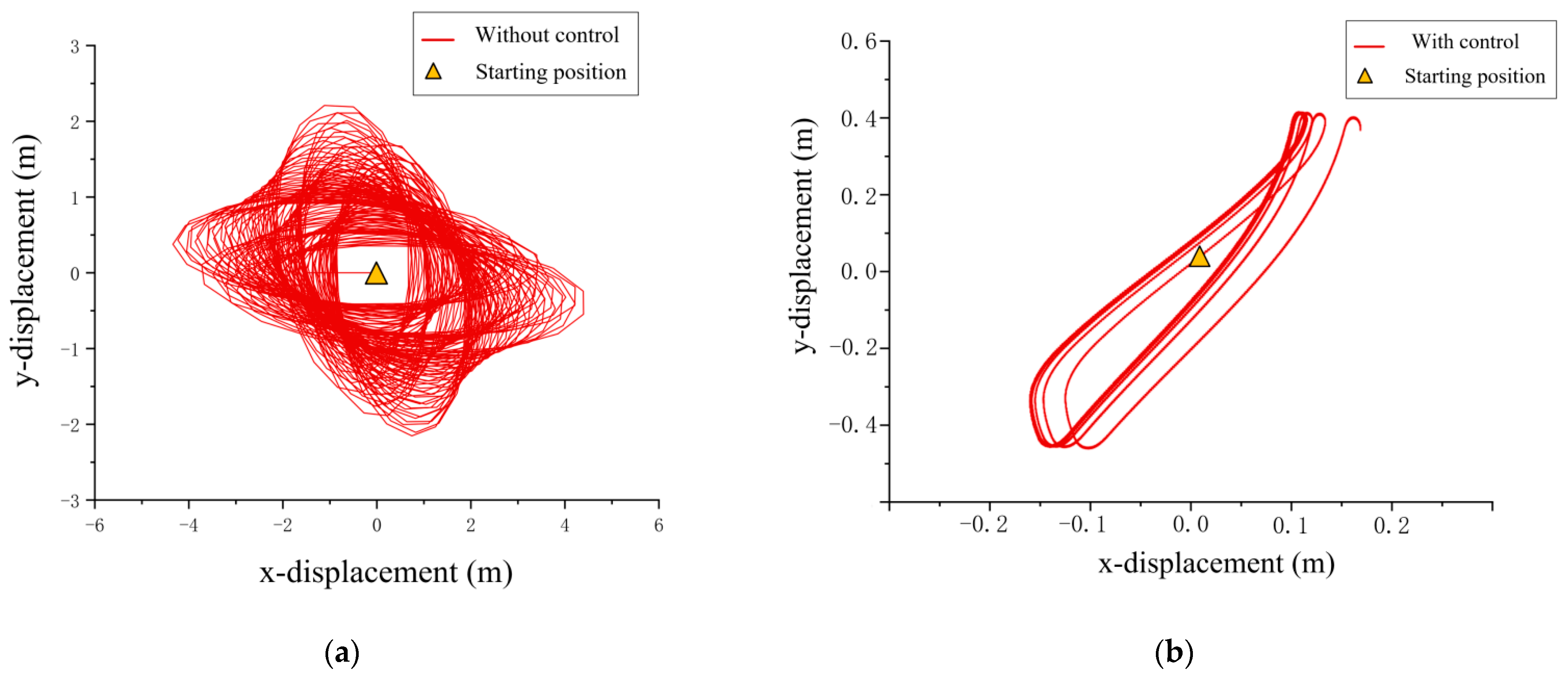
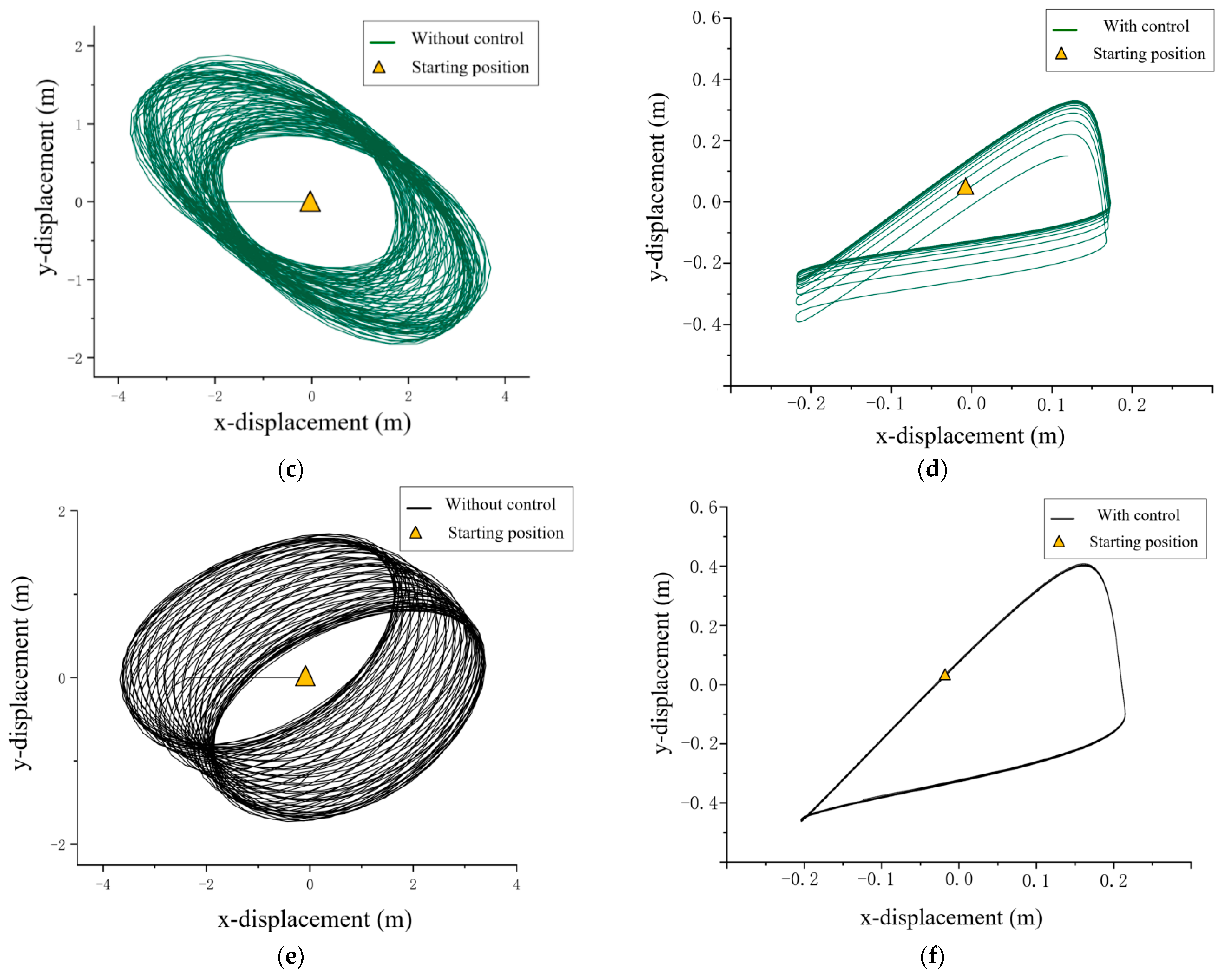
Under irregular environment excitation, the average amplitude of the in-plane angle is reduced by 63%, and that of the out-of-plane angle is reduced by 82% using TTAS. Moreover, the two-dimensional trajectory of the payload is reduced by 92%.

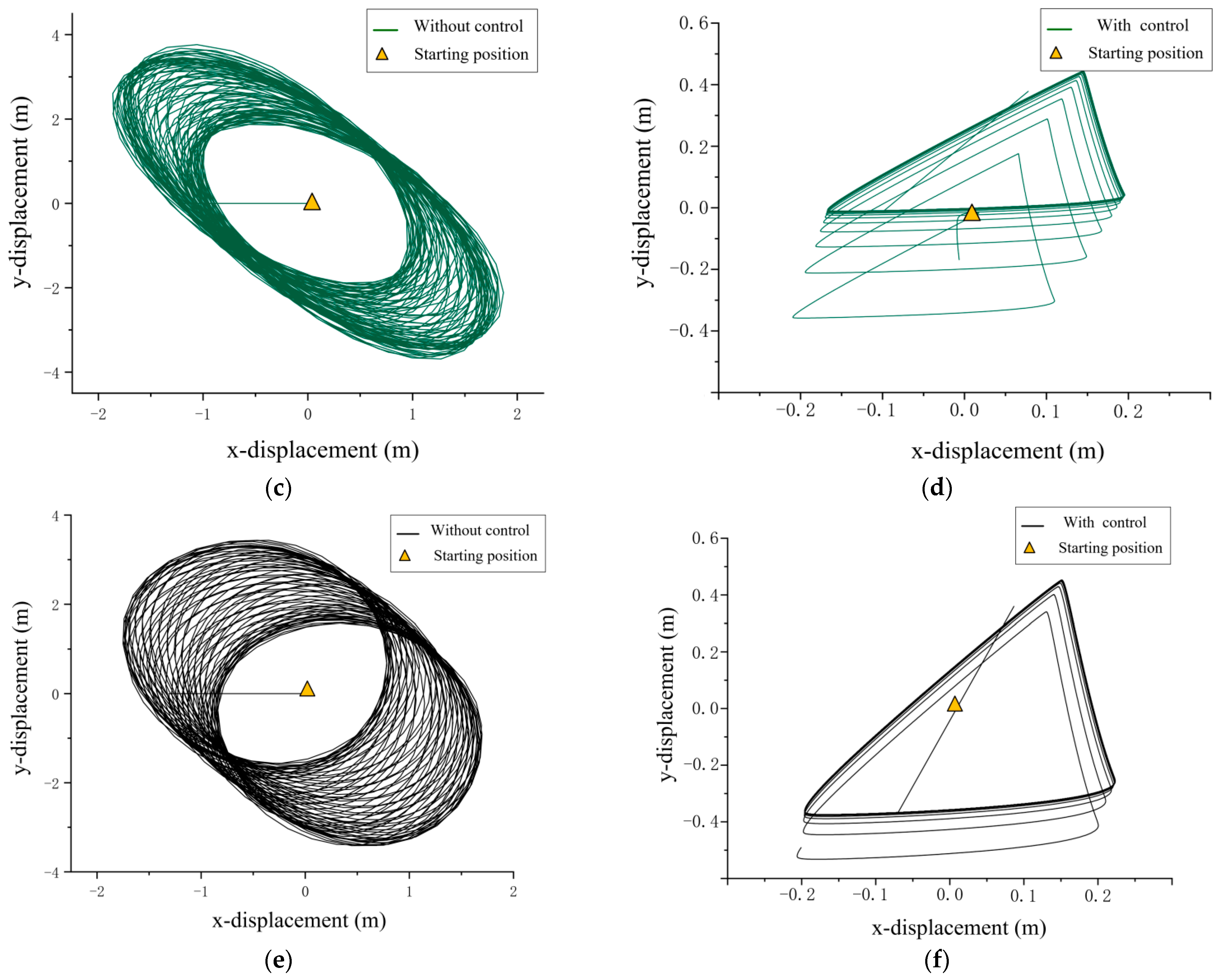
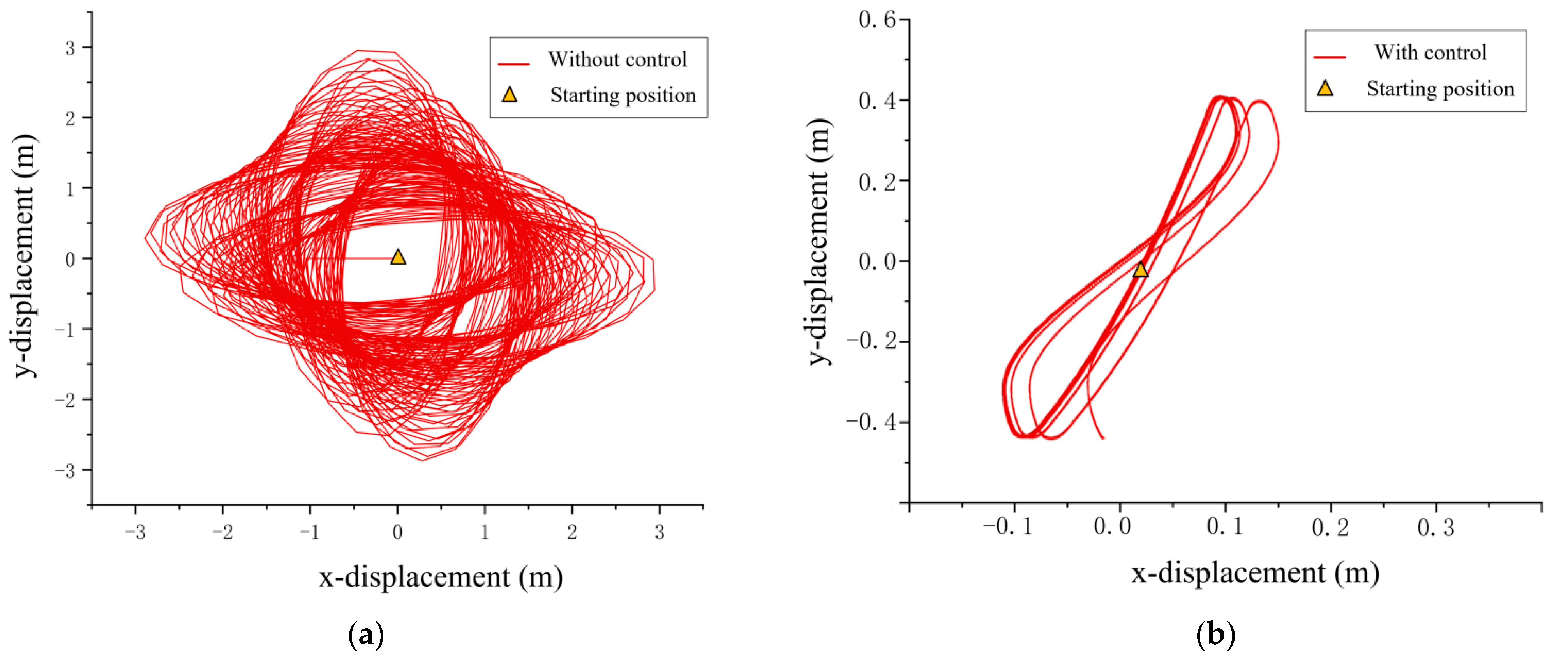
(3)

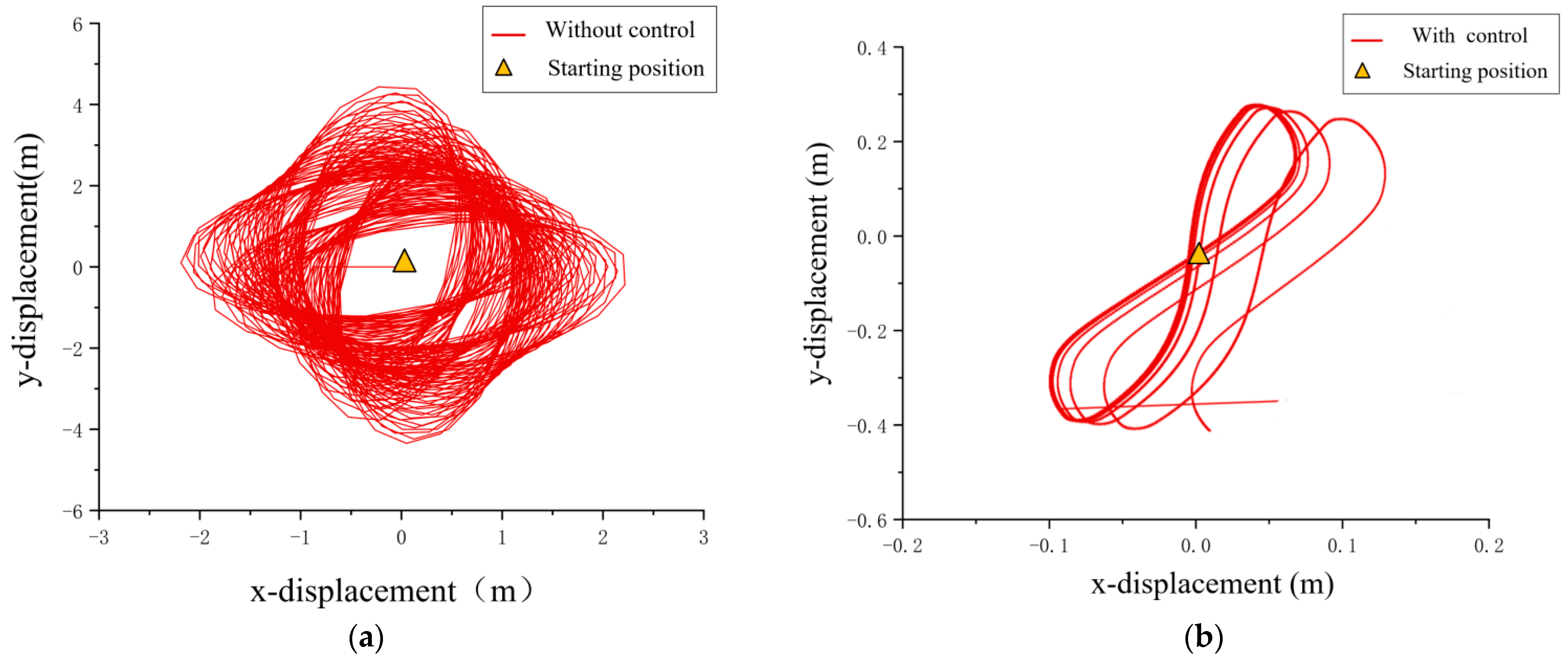
Under regular environment excitation, it was found that the shape of the two-dimensional trajectory of the payload is elliptic without anti-swing control, and it is generally 8-shaped or triangular with anti-swing control. By applying anti-swing control, the two-dimensional trajectory of the payload is reduced by more than 90%.

The dynamic model proposed in this paper can be applied to the prediction of the complex dynamic behavior of TTAS and can be employed to optimize the two-dimensional trajectory of the payload of TTAS. In future work, we will study the trajectory planning of TTAS in limited-space operations and the anti-collision problem of payload lifting in the transport process.

References

1. Smoczek, J.; Szpytko, J.; Hyla, P. The Application of an Intelligent Crane Control System. IFAC Proc. Vol. 2012, 45, 280–285. [Google Scholar] [CrossRef]
2. Chang, C.Y. The switching algorithm for the control of overhead crane. Neural Comput. Appl. 2006, 15, 350–358. [Google Scholar] [CrossRef]
3. Mc, A.; Lta, B. A family of anti-swing motion controllers for 2D-cranes with load hoisting/lowering—ScienceDirect. Mech. Syst. Signal Processing 2019, 133, 106253. [Google Scholar]
4. Belunce, A.; Pandolfo, V.; Roozbahani, H.; Handroos, H. Novel Control Method for Overhead Crane’s Load Stability. Procedia Eng. 2015, 106, 108–125. [Google Scholar] [CrossRef]
5. Tran, Q.; Huh, J.; Nguyen, V.; Kang, C.; Ahn, J.H.; Park, I.J. Sensitivity Analysis for Ship-to-Shore Container Crane Design. Appl. Sci. 2018, 8, 1667. [Google Scholar] [CrossRef]
6. Maghsoudi, M.J.; Ramli, L.; Sudin, S.; Mohamed, Z.; Wahid, H. Improved unity magnitude input shaping scheme for sway control of an underactuated 3D overhead crane with hoisting. Mech. Syst. Signal Process. 2019, 123, 466–482. [Google Scholar] [CrossRef]
7. Yuan, G.H.; Hunt, B.R.; Grebogi, C.; Ott, E.; Kostelich, E.J. Design and Control of Shipboard Cranes. In Proceedings of the ASME 1997 Design Engineering Technical Conferences, Sacramento, CA, USA, 14–17 September 1997. [Google Scholar]
8. Bing, W.; Homaifar, A.; Bikdash, M.; Kimiaghalam, B. Modeling and optimal control design of shipboard crane. In Proceedings of the American Control Conference, San Diego, CA, USA, 2–4 June 1999. [Google Scholar]
9. Kimiaghalam, B.; Homaifar, A.; Bikdash, M. Feedback and feedforward control law for a ship crane with Maryland rigging system. In Proceedings of the American Control Conference, Chicago, IL, USA, 28–30 June 2000. [Google Scholar]
10. Albada, S.B.V.; Albada, G.D.V.; Hildre, H.P.; Zhang, H. A Novel Approach to Anti-Sway Control for Marine Shipboard Cranes. In Proceedings of the 27th Conference on Modelling and Simulation, Ålesund, Norway, 27–30 May 2013. [Google Scholar]
11. Yan, M.; Ma, X.; Bai, W.; Lin, Z.; Li, Y. Numerical Simulation of Wave Interaction with Payloads of Different Postures Using OpenFOAM. J. Mar. Sci. Eng. 2020, 8, 433. [Google Scholar] [CrossRef]
12. Fragopoulos, D.; Spathopoulos, M.P.; Zheng, Y. A pendulation control system for offshore lifting operations-ScienceDirect. IFAC Proc. Vol. 1999, 32, 1475–1480. [Google Scholar] [CrossRef]
13. Ren, Z.; Verma, A.S.; Ataei, B.; Halse, K.H.; Hildre, H.P. Model-free anti-swing control of complex-shaped payload with offshore floating cranes and a large number of lift wires. Ocean Eng. 2021, 228, 108868. [Google Scholar] [CrossRef]
14. Küchler, S.; Mahl, T.; Neupert, J.; Schneider, K.; Sawodny, O. Active Control for an Offshore Crane Using Prediction of the Vessel’s Motion. IEEE ASME Trans. Mechatron. 2011, 16, 297–309. [Google Scholar] [CrossRef]
15. Küchler, S.; Sawodny, O. Nonlinear control of an active heave compensation system with time-delay. In Proceedings of the IEEE International Conference on Control Applications, Yokohama, Japan, 8–10 September 2010. [Google Scholar]
16. Ngo, Q.H. Adaptive sliding mode control of container cranes. Control Theory Appl. IET 2012, 6, 662–668. [Google Scholar] [CrossRef]
17. Kharola, A.; Patil, P.P. Automated Control and Optimisation of Overhead Cranes. Int. J. Manuf. 2017, 7, 41–68. [Google Scholar] [CrossRef]
18. Ismail, R.; That, N.D.; Ha, Q.P. Modelling and robust trajectory following for offshore container crane systems. Autom. Constr. 2015, 59, 179–187. [Google Scholar] [CrossRef]
19. Ku, N.K.; Cha, J.H.; Roh, M.I.; Lee, K.Y. A tagline proportional-derivative control method for the anti-swing motion of a heavy load suspended by a floating crane in waves. Proc. Inst. Mech. Eng. Part M J. Eng. Marit. Environ. 2013, 227, 357–366. [Google Scholar] [CrossRef]
20. Hu, Y.; Tao, L.; Wei, L. Anti-pendulation analysis of parallel wave compensation systems. Proc. Inst. Mech. Eng. Part M J. Eng. Marit. Environ. 2014, 230, 268–271. [Google Scholar] [CrossRef]
21. Martin, I.A.; Irani, R.A. A generalized approach to anti-sway control for shipboard cranes. Mech. Syst. Signal Processing 2021, 148, 107168. [Google Scholar] [CrossRef]
22. Martin, I.A.; Irani, R.A. Dynamic modeling and self-tuning anti-sway control of a seven degree of freedom shipboard knuckle boom crane. Mech. Syst. Signal Process. 2021, 153, 107441. [Google Scholar]
23. Jin, Y.P.; Wan, B.Y.; Liu, D.S.; Peng, Y.D.; Guo, Y. Dynamic analysis of launch & recovery system of seafloor drill under irregular waves. Ocean Eng. 2016, 117, 321–331. [Google Scholar] [CrossRef]
24. Lu, B.; Fang, Y.; Sun, N.; Wang, X. Antiswing Control of Offshore Boom Cranes with Ship Roll Disturbances. IEEE Trans. Control. Syst. Technol. 2017, 26, 740–747. [Google Scholar] [CrossRef]
Figure 1. Schematic diagram of the TTAS.
Jmse 10 01146 g001
Figure 2. Three-dimensional schematic diagram of mechanical structure: 1—ship motion platform; 2—crane housing; 9, 3, and 5—anti-swing knuckle jibs I, II, and III; 10, 4, and 6—taglines I, II, and III; 7—main jib; 8—hoist cable; 11—hook; 12—payload.
Jmse 10 01146 g002
Figure 3. Simplified diagram of the marine crane with TTAS.
Jmse 10 01146 g003
Figure 4. Top view of mechanical structure: (a) top view of three-dimensional mechanical structure; (b) simplified top view of two-dimensional mechanical structure.
Jmse 10 01146 g004
Figure 5. Schematic diagram of statics model: (a) schematic diagram of three-dimensional statics model; (b) stress analysis diagram of two-dimensional statics model.
Jmse 10 01146 g005
Figure 6. Schematic diagram of the dynamic model: (a) schematic diagram of the three-dimensional dynamic model; (b) stress analysis diagram of the two-dimensional dynamic model.
Jmse 10 01146 g006
Figure 7. Ship wet-surface-element mesh.
Jmse 10 01146 g007
Figure 8. Motion response results of six directions (RAO): (a) surge (RAO); (b) sway (RAO); (c) heave (RAO); (d) roll (RAO); (e) pitch (RAO); (f) yaw (RAO).
Jmse 10 01146 g008aJmse 10 01146 g008b
Figure 9. Wave-dip angle diagram.
Jmse 10 01146 g009
Figure 10. The dynamic response of TTAS under the irregular waves. (a) The in-plane angle (θ) of the payload in the irregular waves; (b) in the irregular waves, the out-of-plane angle (Ψ) of the payload; (c) the x, y displacement of the payload without control; (d) the x, y displacement of the payload with control.
Jmse 10 01146 g010
Figure 11. The dynamic response of TTAS under Condition 1. (a) The x, y displacement without control of the payload when the hoist cable is 0.6 m; (b) the x, y displacement with control of the payload when the hoist cable is 0.6 m; (c) the x, y displacement without control of the payload when the hoist cable is 1.2 m; (d) the x, y displacement with control of the payload when the hoist cable is 1.2 m; (e) the x, y displacement without control of the payload when the hoist cable is 1.8 m; (f) the x, y displacement with control of the payload when the hoist cable is 1.8 m.
Jmse 10 01146 g011aJmse 10 01146 g011b
Figure 12. The dynamic response of TTAS under Condition 2. (a) the x, y displacement without control of the payload when the hoist cable is 0.6 m; (b) the x, y displacement with control of the payload when the hoist cable is 0.6 m; (c) the x, y displacement without control of the payload when the hoist cable is 1.2 m; (d) the x, y displacement with control of the payload when the hoist cable is 1.2 m; (e) the x, y displacement without control of the payload when the hoist cable is 1.8 m; (f) the x, y displacement with control of the payload when the hoist cable is 1.8 m.
Jmse 10 01146 g012aJmse 10 01146 g012b
Figure 13. The dynamic response of TTAS under Condition 3. (a) The x, y displacement without control of the payload when the hoist cable is 0.6 m; (b) the x, y displacement with control of the payload when the hoist cable is 0.6 m; (c) the x, y displacement without control of the payload when the hoist cable is 1.2 m; (d) the x, y displacement with control of the payload when the hoist cable is 1.2 m; (e) the x, y displacement without control of the payload when the hoist cable is 1.8 m; (f) the x, y displacement with control of the payload when the hoist cable is 1.8 m.
Jmse 10 01146 g013aJmse 10 01146 g013b