Article

Prediction Method for Ocean Wave Height Based on Stacking Ensemble Learning Model

1
School of Automation, Wuhan University of Technology, Wuhan 430070, China
2
CSSC Marine Technology Co., Ltd., Shanghai 200136, China
*
Author to whom correspondence should be addressed.
J. Mar. Sci. Eng. 2022, 10(8), 1150; https://doi.org/10.3390/jmse10081150
Submission received: 5 July 2022 / Revised: 8 August 2022 / Accepted: 15 August 2022 / Published: 19 August 2022
(This article belongs to the Topic Wind, Wave and Tidal Energy Technologies in China)

Abstract

:
Wave heights are important factors affecting the safety of maritime navigation. This study proposed a stacking ensemble learning method to improve the prediction accuracy of wave heights. We analyzed the correlation between wave heights and other oceanic hydrological features, according to eleven features, such as measurement time, horizontal velocity, temperature, and pressure, as the model inputs. A fusion model consisting of two layers was established according to the principle of stacking ensemble learning. The first layer used the extreme gradient boosting algorithm, a light gradient boosting machine, random forest, and adaptive boosting to determine the deep relations between the wave heights and the input features. The second layer used a linear regression model to fit the relation between the first layer outputs and the actual wave heights, using the data from the four models of the first layer. The fusion model was trained based on the 5-fold cross-verification algorithm. This paper used real data to test the performances of the proposed fusion model, and the results showed that the mean absolute error and the mean squared error of the fusion model were at least 35.79% and 50.52% better than those of the four models.

1. Introduction

In recent years, with China’s Maritime Silk Road strategy and the Blue Water Navy national defensive strategy proposed [1,2,3], the shipping industry and marine research have developed rapidly, and the research on maritime navigation safety has been of great significance in China’s development [4,5]. Approximately 60% of maritime navigation accidents have been caused by unnatural factors, such as collisions and machine failures, and 40% have been caused by bad weather [6,7]. Marine climatic conditions are complex and changeable, and avoiding dangerous waves is critical for human safety. When the wave height reaches more than 4 m, it is regarded as a catastrophic wave and can overturn navigation ships, destroy coastal engineering structures, and significantly increase the danger of maritime activities. Therefore, accurate wave predictions are needed to ensure safety.
To improve the performance of wave prediction models, researchers have employed many different prediction methods, including empirical models, numerical simulations [8], and machine-learning methods. Based on empirical models, waves have been predicted by using the hypothesis of prior models, such as the auto-regression and moving average model. Based on numerical models, such as the wave model, the wave features have been predicted by the wave spectrum control equation. Machine-learning methods have attracted attention due to their rapid computing speed and large data capacity, and machine-learning models, such as artificial neural networks [8,9,10,11,12,13,14], fuzzy systems [8,15,16], and genetic algorithms [17,18,19], have been used in wave predictions, effectively improving the performance of prediction models. Based on machine-learning algorithms, the support vector machine [20,21,22,23,24] has been widely used in the prediction of marine environment elements of ship navigation safety and coastal engineering meteorological hydrology. Mahjoobi et al. [25] used the support vector regression algorithm to establish a prediction model for the effective height of waves, and they used the ocean surface wind speed as the input characteristic data. The experiment indicated that the method had a high prediction accuracy and rapid calculation speed in predicting the effective wave height. Zhu et al. [26] used the back propagation neural network algorithm to predict the effective wave height and the average wave direction. Sinha et al. [27] used a genetic algorithm to predict the wave height of the Bay of Bengal, and the results showed that the timeliness performance of the algorithm was better. Nikoo et al. [28] proposed, for the first time, to use artificial immune recognition systems for the prediction of effective wave heights in Lake Superior in the northern United States, and their prediction performance was better than that of the artificial neural networks, such as Bayesian networks and support vector machines. Wu et al. [29] proposed an ocean temperature prediction method that integrated an empirical modal decomposition algorithm and a back propagation neural network, and it obtained the final prediction result by aggregating the prediction data of each series of intrinsic pattern functions, and the experiment analysis showed that the model could effectively predict the ocean temperature of the time series. Ali et al. [30] utilized an improved limit learning machine model, and it regarded the historical lag sequence of effective wave heights in the model to predict the future effective wave heights, and the model was more accurate. James et al. [31] used multilayer perceptron and support vector machines to perform regression analysis of wave heights and classification analysis of feature periods, and the results showed that the prediction performances of the two machine-learning models were good, with a rapid calculation speed.
The aforementioned prediction models based on machine-learning algorithms have obtained good performance in predicting marine hydrological characteristics. Therefore, it was of great significance to use machine-learning algorithms to construct a prediction model for ocean wave heights, and it was meaningful to conduct further study to improve the accuracy of the model. Based on machine-learning models, this study used a multi-model prediction method based on ensemble learning [32,33,34,35,36]. Firstly, we analyzed the linear and nonlinear relationship between ocean waves and ocean hydrological features according to the formation mechanism of ocean waves, and then, the important factors of waves were obtained as inputs for the model. This method effectively combined four proven learning algorithms through the multi-model stacking method. By comparing and analyzing the prediction performance of four single models and that of the fused model, the prediction effects of the stacking ensemble learning model on ocean wave height were investigated. This method effectively improved the stability of the prediction model without overfitting, improved the accuracy of the wave prediction results, and indicated the potential for meteorological predictions and route planning for maritime navigation.
This paper is organized as follows. Section 2 introduces the method for establishing the multi-model stacking method. Section 3 details the proposed prediction method of ocean wave height based on the stacking ensemble learning model. The experiment results and analysis are contained in Section 4. Section 5 summarizes the conclusions.

2. Materials and Method Analysis

2.1. Experimental Data Source

Located south of China’s mainland, the South China Sea is one of China’s three marginal oceans, and it is rich in offshore oil and gas mineral resources, but it is currently difficult to accurately predict the ocean waves in this area. With the rapid development of China’s economy and the rapid enhancement of military strength, the need to predict ocean waves in the South China Sea is becoming increasingly urgent. In this paper, the intermediate ocean areas of the Paracel Islands and Hainan in the South China Sea were selected as the prediction areas, and the relevant data of the training model were based on the dataset downloaded from the European Centre for Medium-Range Weather Forecasts (ECMWF). The observation data coordinates were (110°50′′ E, 17°75′′ N), the time resolution was one hour, and the time interval was from 1 January 2020 to 31 December 2020. The area is located in the inland fortress of the South China Sea, surrounded by a variety of ocean routes, and it was representative of ship route planning to avoid dangerous ocean winds and waves. Since the excessive height of the waves can pose a danger to the safety of a sailing vessel, hmax was the prediction target, and according to the formation cause and propagation principle of ocean waves, the meteorological and hydrological factors that could affect the maximum height of the waves were selected as the characteristic data, and they were u10, v10, airMass, cdww, vertV, mpww, msl, wind, sst, and sp. The detailed descriptions are provided in Table 1.
The hmax was the prediction target, and the remaining ten meteorological and hydrological features were part of the basic features of the model. Table 2 presents the minimum values, maximum values, and median values of individual features. As we can see, some features are vectors, while some are scalars, and some features have large numerical values, while some features have values that are too small. Data normalization is therefore required.

2.2. XGBoost Algorithm

There are some machine learners in Table 3. The XGBoost algorithm is a tree algorithm based on boosting iterative machine learning [37,38], and it is suitable for solving classification and regression problems. Additionally, the objective function model can be written as follows:
y ^ i = ϕ ( x i ) = k = 1 K f k ( x i ) , f k
In Equation (1), y ^ i is the prediction value for the training sample i , f is a function in the function sets , and is the sets of all the regression trees in the model; K is the number of all the regression trees in the model. The objective equation of the algorithm can be written as follows:
( t ) = i n l ( y i , y ^ i ( t 1 ) + f t ( x i ) ) + Ω ( f t )
In Equation (2), f t is continuously added to help minimize the goal, y ^ i ( t 1 ) is the prediction value for the training sample i at the time of the ( t 1 ) iteration, l ( y i , y ^ i ( t 1 ) ) is the training loss function of the model, and Ω is the regularization term.

2.3. LightGBM Algorithm

The LightGBM is a decision tree algorithm based on histograms [39]. It uses a histogram algorithm to solve the problem of merging mutually exclusive features.
As shown in Figure 1, most of the learning algorithms for decision trees use a level-wise strategy to grow trees, which splits leaves of the same layer at once and treats leaves of the same layer equally. However, many leaves have low splitting gain and do not need to split, thereby reducing the running efficiency of the model and increasing memory loss. LightGBM grows trees by a leaf-wise strategy. Each split will find the leaf with the greatest split gain from all the current leaves and then split it. This can reduce more errors and result in better accuracy.

2.4. Random Forest Algorithm

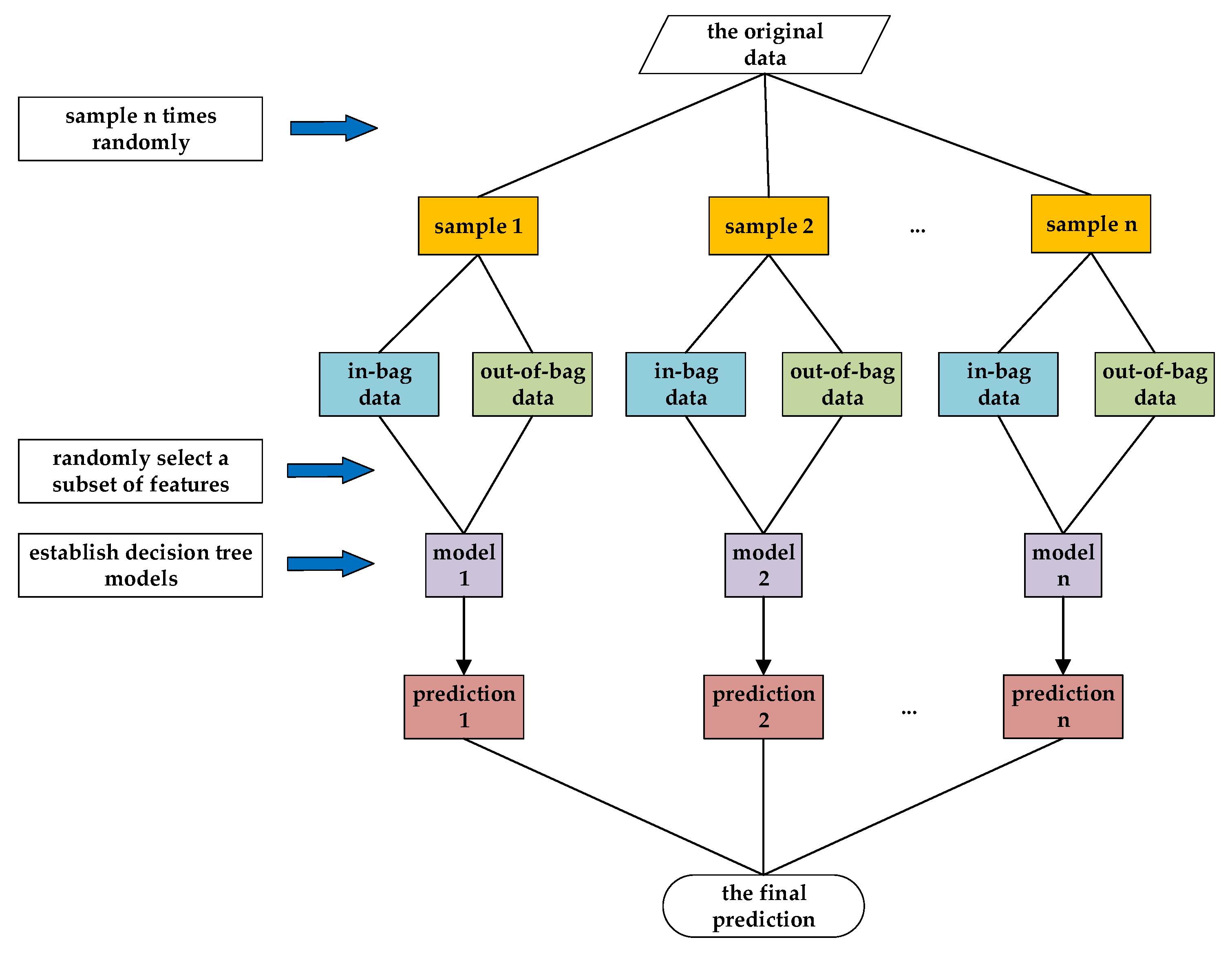
The RF is an ensemble learning algorithm based on decision trees [39]. Figure 2 is a schematic diagram of the topology as an optimization improvement of the decision tree algorithm. It combines multiple decision trees, and the establishment of each tree model is based on independent sample data. The specific steps of the algorithm are as follows:
  • Self-service sampling;
  • Determine the optimal number of features of the decision tree;
  • Establish a random forest algorithm model.
The in-bag data are used for the generation of the decision tree, while the out-of-bag data are used to determine the optimal number of features of the decision tree. Additionally, the average method is used to take the mean of all decision trees as the output, and the output equation of the model is as follows:
G ( x ) = 1 n i = 1 n g i ( x )
In Equation (3), g i ( x ) is the prediction value of every decision tree, and n is the number of decision trees.

2.5. AdaBoost Algorithm

The AdaBoost algorithm [40], a boosting method proposed by Yoav Freund and Robert Schapire in 1995, is a combination of multiple weak learners into a single strong learner. The sample weights will be updated until the model reaches its prediction accuracy requirements or the specified maximum number of iterations. The specific steps of the algorithm are as follows:
  • Initialize the weight distribution of the training data;
  • Train the learners and calculate the error parameters;
  • Update sample weights;
  • Obtain the final algorithm model.
In step 1, the input sample set is T = { ( x 1 , y 1 ) , ( x 2 , y 2 ) , , ( x N , y N ) } , and the weak learners are cart regression trees, while the number of weak learner iterations is K . Supposing that there are N samples, and the initial weight of each training sample point is 1 / N . The initial weight distribution is shown as follows:
D 1 = ( ω 11 , , ω 1 i , , ω 1 N ) , ω 1 i = 1 N , i = 1 , 2 , , N
In step 2, the learner numbered m ( m = 1 , 2 , , M ) will use a training dataset with the weight distribution D m to perform the learning, obtaining the base learner prediction function G m ( x ) . It calculates the maximum error on the training dataset as follows:
E m = max | y i G m ( x i ) | , i = 1 , 2 , , N
Then, it calculates the relative error for each sample as follows:
e m i = | y i G m ( x i ) | E m
The error rate of the weak learner numbered m is finally obtained as follows:
e m = i = 1 N ω m i e m i
The weak learner weight coefficient is obtained as follows:
α m = e m 1 e m
In step 3, in the specific training process, according to the error index analysis of the above-mentioned base learner on the training sample, the prediction accuracy is judged to meet the requirements and then to update the weight of the sample accordingly. The weight distribution for the updated sample set is as follows:
ω m + 1 , i = ω m i z m α m 1 e m i
The normalization factor in Equation (9) is as follows:
Z m = i = 1 N ω m i α m 1 e m i
In step 4, the set of samples will be used to train the next weak learner, and the entire training process will be iteratively performed in a loop, as in the above steps. After sample training, the weak learner with a small prediction error has a large right to speak and plays a significantly decisive role in the final model prediction function. Finally, the weak learners are combined into a new strong learner by the weak learner weight coefficient, and the model equation of the strong learner obtained by using the weighted average method is as follows:
f ( x ) = m = 1 M ( ln 1 a m ) G m ( x )

3. Experimental Steps and Model Building

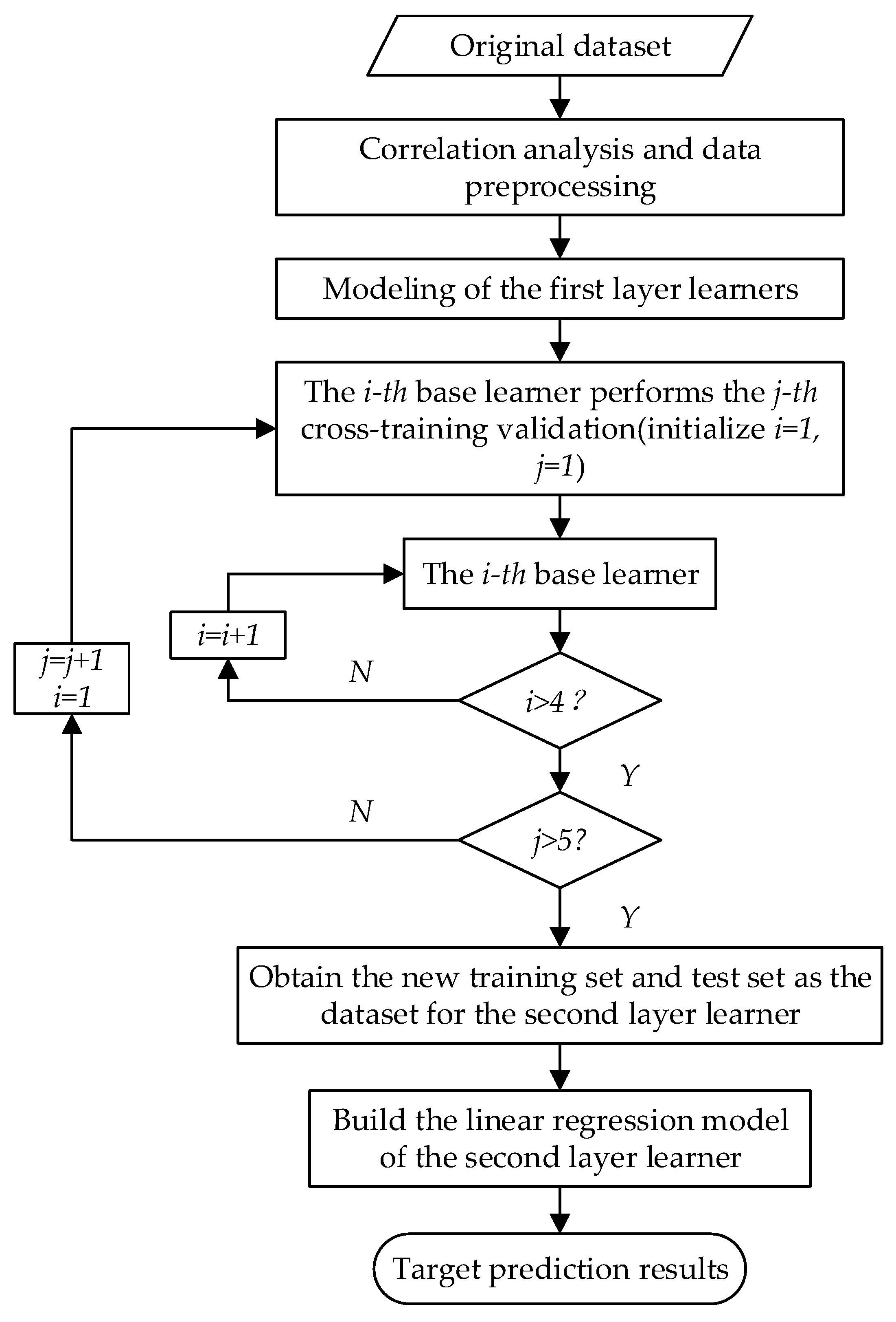
The modeling process of the proposed method is shown in Figure 3. There are four base learners in the first layer, and the base learners choose a 5-fold cross-verification to establish the proposed model.

3.1. Data Preprocessing

Data normalization is a common data preprocessing operation, and it processes data of different sizes and dimensions and scales them to the same interval range. Due to the large fluctuation of data characteristics and the difference in dimensions, the maximum and minimum normalization method was selected for the standardization of data characteristics, and it could not only normalize the data into a certain range but also better maintain the original data structure. The normalization equation is as follows:
x ¯ i = x i min ( x i ) max ( x i ) min ( x i )
In Equation (12), x i and x ¯ i are, respectively, the values before and after the normalization of the marine hydrological characteristic variables; max ( x i ) and min ( x i ) , respectively, represent the maximum and minimum values of the variables. After the normalization process, the original data were linearly converted to the range of (0,1), which sped up the convergence speed of the model algorithm and reduced the model error, to a certain extent.

3.2. Data Analysis

The first day of each month in 2020 was chosen to observe the daily change in hmax. As shown in Figure 4, the wave height showed a daily downtrend at night in Figure 4a,b, but it was more stable in Figure 4c,d. It did not reach one meter
On 1 September, while it was more than seven meters on 1 December. The analysis indicated that seasonal change was also an important influencing factor in predicting wave height, so the time range for experimental data was one year, and the model can include all different seasons in the experiment. Based on the influence of different daily observation times on the wave height and the daily changes, the observation time was divided into hours as an input feature.
The observation time and ten meteorological and hydrological features were determined as the features of the proposed model, and hmax was used as the prediction target. The distribution maps of several meteorological hydrological features and the regression plot with the target feature are shown in Figure 5; if the data could conform to the normal distribution, all the points would be in a straight line. The degree of normal distribution of wind was the highest, and it had the highest linearity with the predicted target. While this degree of sst was lower, the point distribution in the regression graph of the prediction target was more dispersed and farther away from the regression line.

3.3. Establishment of Stacking Model

Stacking is a multi-model fusion ensemble learning algorithm proposed by Wolpert [41]. It improved the accuracy of the model by fusing the base learner model. In the stacking hierarchical model framework, the basic learner is called the first-layer learner, and the composite learner is called the second-layer learner. The first layer consisted of multiple base learners that performed the training and predictions on the original dataset, and the second layer regarded the output of the first layer as input features, while the target values of the original data were seen as those of the new features. The second-layer model was trained through the new dataset to obtain a complete two-layer stacking model. The stacking algorithm pseudocode is shown in Algorithm 1.
Algorithm 1: The stacking algorithm pseudocode.
Stacking model algorithm
initialization: Set the first layer learner: m o d e l 1 ,   m o d e l 2 ,   ,   m o d e l K .
        the second-layer learner: m o d e l .
data input  T = { ( x 1 , y 1 ) , ( x 2 , y 2 ) , , ( x N , y N ) }
for  k = 1 , 2 , , K
   f k = m o d e l k ( T )
end
T = ϕ
for  n = 1 , 2 , , N
  for  k = 1 , 2 , , K
       z n k = f k ( x n )
  end
   T = T ( ( z n 1 , z n 2 , z n K ) , y n )
end
f = m o d e l ( T )
model output  F ( x ) = f ( f 1 ( x ) , f 2 ( x ) , , f K ( x ) )
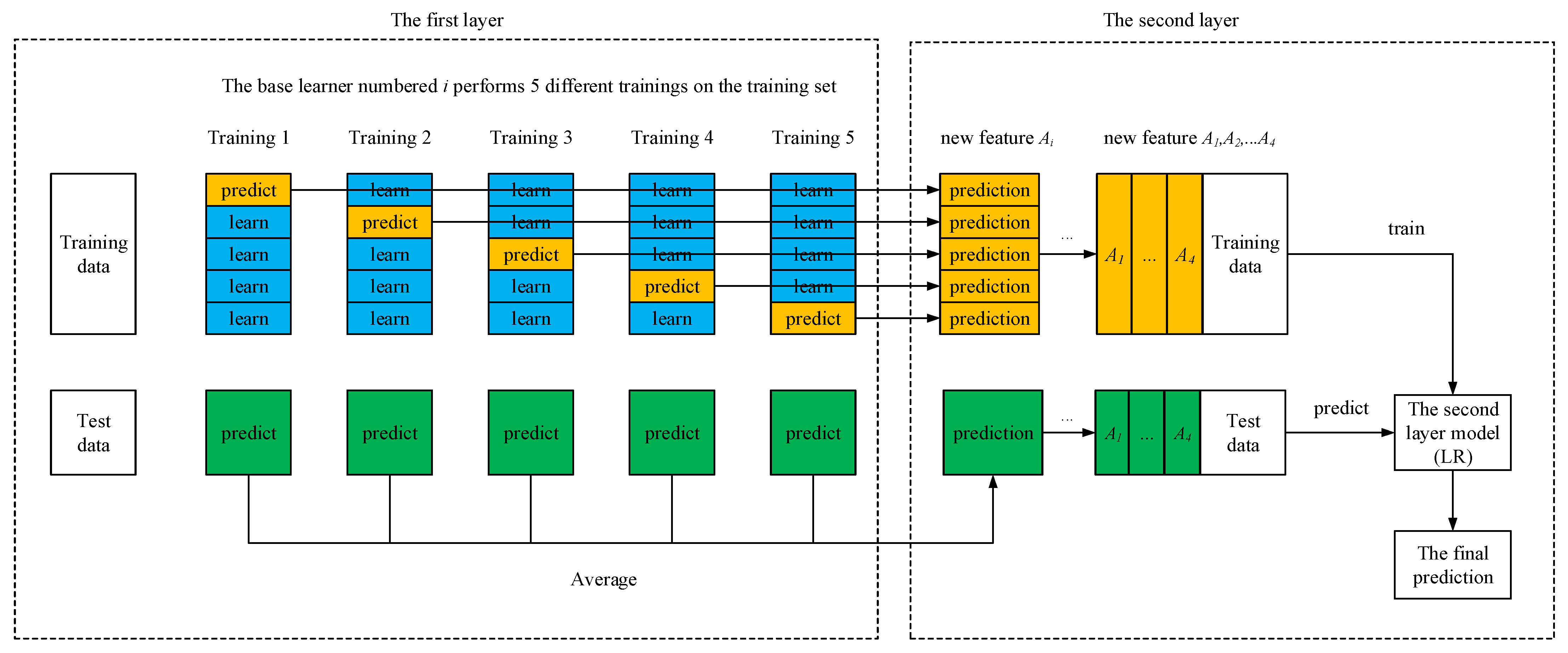
In this paper, the stacking algorithm based on the 5-fold cross-validation was used to establish a wave height prediction model, and its principle is shown in Figure 6. The specific implementation steps were as follows:
  • Choice of learners;
  • Division of the first-layer dataset;
  • Training and prediction of the first-layer base model;
  • Dataset of the second-layer learners;
  • Training and prediction of the second-layer learners.
The first layer selected a strong learner as the base model, and it selected XGBoost, LightGBM, RF, and AdaBoost. The second-layer base model selected a simple regressor to prevent overfitting and used the LR algorithm.
In step 2, to strengthen the robustness of the model, the first-layer base model would be trained for multiple sets of different training sets. The original training set was split into k equal parts, one of which was used as the verification set in turn, and the remaining ( k 1 ) part was used as the training set of the base learner. The value k was five in this paper.
As shown in Figure 6, each base learner performed five model pieces of training on the training set, and it used the 5-fold cross-validation. For example, when performing Training 1, the base model was trained with the last four parts of the data, and the first part was used as the verification data of the model, and the corresponding prediction values were obtained by predicting the validation data. Five model pieces of training were performed in turn, and each base model obtained five predictions of the testing data and five predictions of the test set.
The prediction values of five parts from the training data were merged vertically, and each base learner obtained a new feature, and they were A1, A2, A3, and A4. The training set of the second layer was composed of the new feature set and the target value of the original data. The five test data prediction values of each base learner were averaged as the value of the new feature, and then, the average feature set and the target values of the original test data were combined to form the test set of the second layer.

4. Results and Discussion

4.1. Model Evaluation and Analysis

The meteorological and hydrological feature datasets were from 1 January to 31 December 2020—a total of 8784 h and 8784 rows of data—and 70% of them were used as training sets, while the remaining 30% were used as test sets. The regression prediction model evaluation was performed according to the following three indicators: (1) The mean absolute error (MAE) was used to assess the proximity of the predicted and true values; (2) The mean squared error (MSE) was the mean sum of the squares of the errors of the sample points corresponding to the fitted data and the original data; (3) The r2 score (R2) characterized the degree of fit of the model to the data. The calculation equations are as follows:
MAE = 1 n i = 1 n | y i y ^ i |
M S E = 1 n i = 1 n ( y i y ^ i ) 2
R 2 = 1 i = 1 n ( y i y ^ i ) 2 i = 1 n ( y i y ¯ ) 2
In the above equation, y i , y ^ i   , and y ¯ , respectively, represent the real value, the predicted value, and the average value of the samples; n is the sample size.
In the process of training and extracting predictions in the first-layer base learner, the optimization parameters of each algorithm were obtained by grid search. The grid search provided a list of values for each parameter to be optimized and iterated over all combinations of values in the list to obtain the optimal combination of parameters, and it was more accurate than a random search. In the XGBoost model, when the maximum depth of the parameter decision tree was 3, and the number of trees was 30, the model had the best score of 0.889. Similarly, the optimal parameters of every single model were obtained, and the test set was applied to the trained model to verify the prediction evaluation of each model. In Table 4, the first layer of the base model, the single model established by the AdaBoost algorithm, had a better prediction performance both in the training set and the test set, and it had a higher accuracy with its R2, reaching 0.920. However, its prediction accuracy in the training set was a little better than that in the test set.
To further analyze the predictive ability of the base learner, Table 5 reflects the accuracy and fit of the model predictions. Respectively, (1) corr was the correlation value between the real value and the predicted value of the model, and the closer it was to 1, the better; (2) std_resid was the variance between the true value and the predicted value of the model, and the smaller it was, the more stable the model would be; (3) the number of z > 3 in the sample, and the larger it was, the greater the sample bias in the prediction. The calculation equations are as follows:
c o r r = i = 1 n ( y ^ i p ¯ ) ( y i y ¯ ) i = 1 n ( y ^ i p ¯ ) 2 i = 1 n ( y i y ¯ ) 2
s t d _ r e s i d = 1 n 1 i = 1 n ( y i y ^ i ) 2
z = i = 1 n ( y i y ^ i ) 1 n i = 1 n ( y i y ^ i ) s t d _ r e s i d
In the above equations, y i , y ^ i   , y ¯ , and p ¯ , respectively, represent the real value, the predicted value, the average of the real value, and the average of the predicted value; n is the sample size.
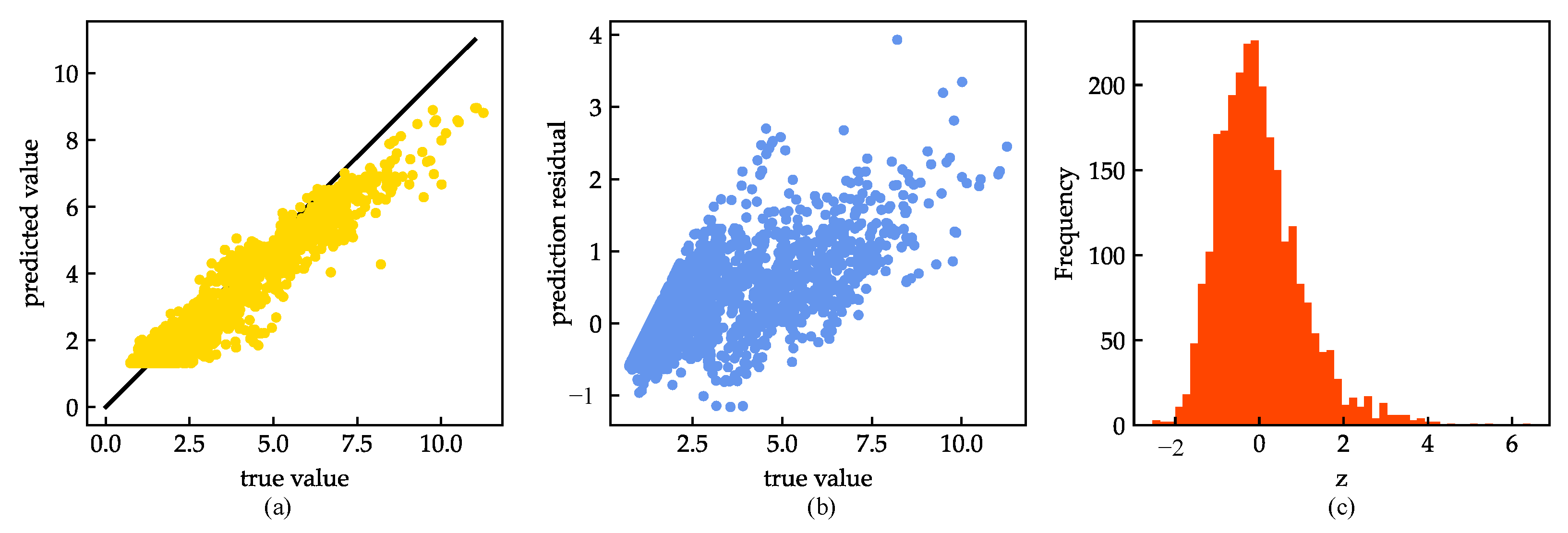
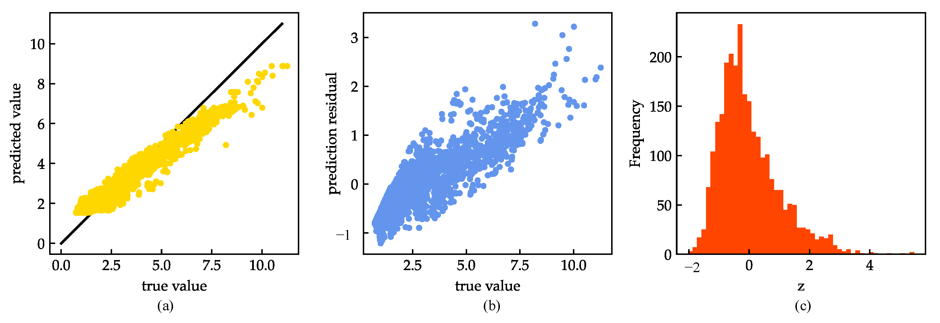
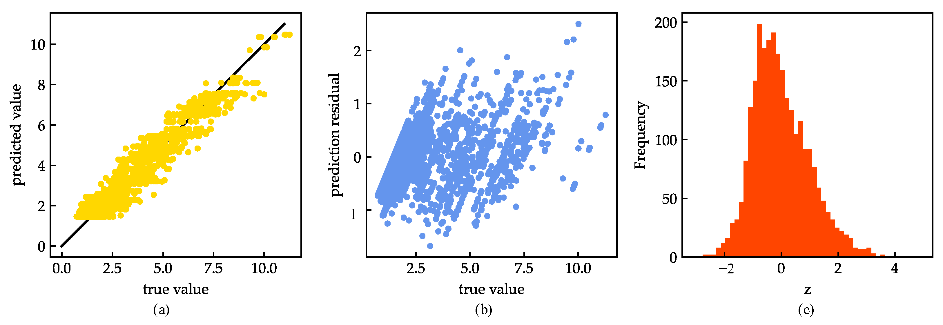
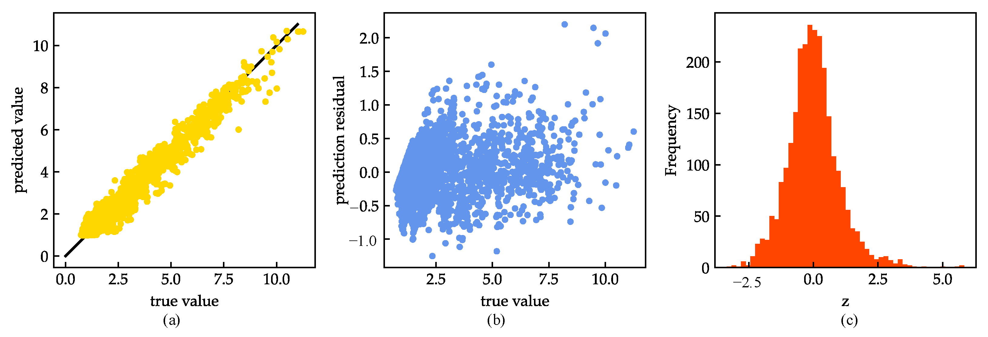
The corr of the AdaBoost prediction model was 0.962, the std_resid was 0.521, and the sample number of z > 3 was 12, indicating that the model had better predictive performance. In Figure 7, Figure 8, Figure 9 and Figure 10, when the true value exceeded 8, there was a large deviation in the model prediction value. Therefore, the prediction accuracy of the single model reduced gradually when the wave values increased. The prediction performance of all base models on the test set was worse than that on the training set, but the stacking model was improved on the test set, and no overfitting occurred. Moreover, the prediction performance of the stacking model on the test set was better than that of every single model, and the model evaluation parameters MAE, MSE, and R2 were 35.79%, 50.52%, and 4.34% higher, respectively, than the single model with the best performance, indicating that the stacking model of the multi-model fusion framework improved the generalization performance of the model, so the proposed model had higher reliability and accuracy in wave prediction.

4.2. Model Improvements

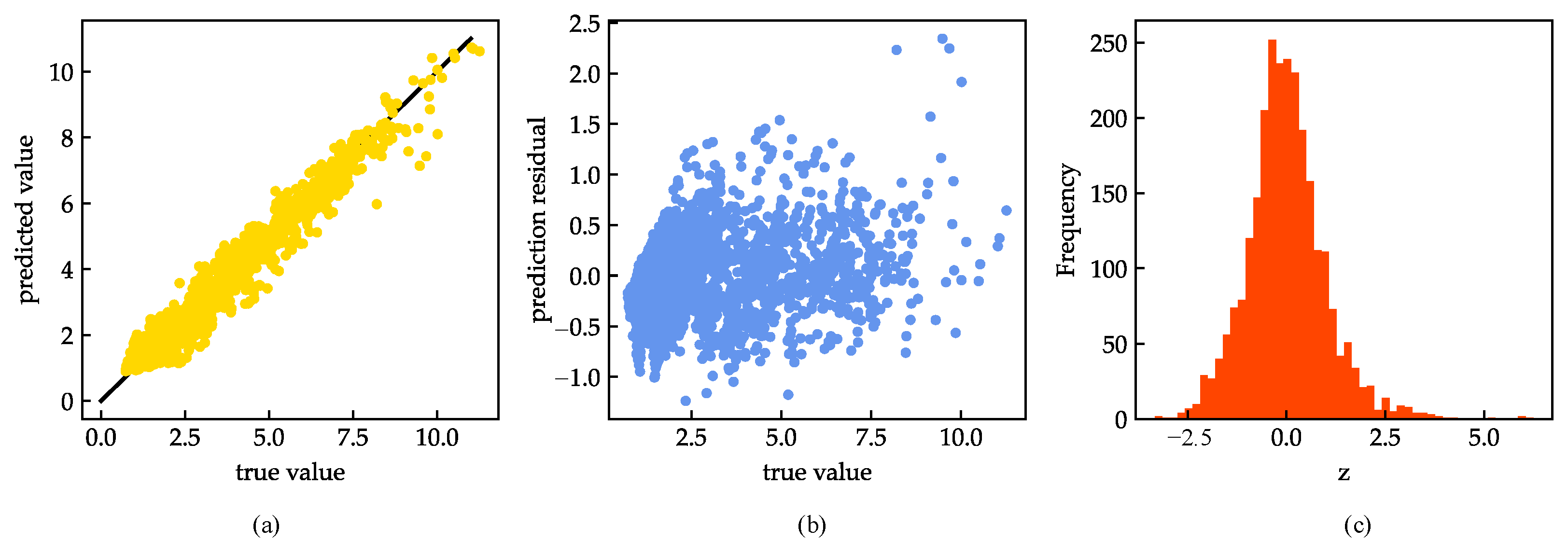
In the process of the stacking model fusion, the new features and the original features were combined as the dataset of the second-layer model, which not only included the feature information of the original data but also added new features from the first layer. It had higher prediction accuracy and did not have model overfitting. In Table 4 and Figure 11 and Figure 12, the prediction performance of the improved stacking model was improved on both the training set and the test set, and its parameters MSE and R2 were 0.709% and 0.104% better, respectively, than the original stacking model on the test set. The stacking models also provided a good prediction performance when the wave height was over 8 m. This indicated that the proposed method enhanced the stability of the model.

5. Conclusions

Based on the wave height, the objective of this study was to establish a high-precision and robust prediction model. Firstly, to ensure the quality of the model data, the original data of marine features were analyzed and pre-processed, and a high-quality marine feature dataset was obtained. In order to ensure the accuracy of modeling, the optimal parameter combinations of four base learners were obtained by using a grid search optimization. It combined stacking multi-model fusion with ensemble learning algorithms, and a wave height prediction method was proposed. The prediction performance of the model analysis was performed on the training and test sets. Among the four single models, the AdaBoost model had a higher accuracy with its R2, reaching 0.920 in both sets. Additionally, the MAE, MSE, and R2 of the fusion model were 35.79%, 50.52%, and 4.34% better than the AdaBoost model. The results showed that the proposed model had better prediction performance and good model robustness.

Author Contributions

Conceptualization, Y.Z. and H.Z.; methodology, Y.Z.; software, Y.Z.; validation, Y.Z. and H.Z.; formal analysis, Y.Z.; investigation, G.L.; resources, J.L.; data curation, J.L.; writing—Original draft preparation, Y.Z.; writing—Review and editing, Y.Z.; visualization, Y.Z.; supervision, H.Z.; project administration, H.Z.; funding acquisition, H.Z. All authors have read and agreed to the published version of the manuscript.

Funding

This research received no external funding.

Institutional Review Board Statement

Not applicable.

Informed Consent Statement

Not applicable.

Data Availability Statement

Not applicable.

Conflicts of Interest

The authors declare no conflict of interest.

References

  1. Liu, Z. Towards the “Blue Water Navy”. Xinmin Weekly 2017, 35, 58–59. [Google Scholar]
  2. Wan, F.; Liu, Y.; Chen, W. The Design of Regional Cultural Service of the Maritime Silk Road Based on Symbolic Semantics. Front. Art Res. 2022, 4, 1–6. [Google Scholar] [CrossRef]
  3. Song, A.Y.; Fabinyi, M. China’s 21st century maritime silk road: Challenges and opportunities to coastal livelihoods in ASEAN countries. Mar. Policy 2022, 136, 104923. [Google Scholar] [CrossRef]
  4. Daniel, D.; Ryszard, W. The Impact of Major Maritime Accidents on the Development of International Regulations Concerning Safety of Navigation and Protection of the Environment. Sci. J. Pol. Nav. Acad. 2017, 211, 23–44. [Google Scholar]
  5. Poznanska, I.V. Organizational-Economic Aspects of the Implementation of International Standards for Safety of Maritime Navigation. Probl. Ekon. 2016, 3, 68–73. [Google Scholar]
  6. Rolf, J.B.; Asbjørn, L.A. Maritime navigation accidents and risk indicators: An exploratory statistical analysis using AIS data and accident reports. Reliab. Eng. Syst. Saf. 2018, 176, 174–186. [Google Scholar]
  7. Hanzu-Pazara, R.; Varsami, C.; Andrei, C.; Dumitrache, R. The influence of ship’s stability on safety of navigation. IOP Conf. Ser. Mater. Sci. Eng. 2016, 145, 082019. [Google Scholar] [CrossRef]
  8. Mahjoobi, J.; Etemad-Shahidi, A.; Kazeminezhad, M.H. Hindcasting of wave parameters using different soft computing methods. Appl. Ocean. Res. 2008, 30, 28–36. [Google Scholar] [CrossRef]
  9. Deo, M.C.; Jha, A.; Chaphekar, A.S.; Ravikant, K. Neural networks for wave forecasting. Ocean Eng. 2001, 28, 889–898. [Google Scholar] [CrossRef]
  10. Makarynskyy, O. Improving wave predictions with artificial neural networks. Ocean Eng. 2003, 31, 709–724. [Google Scholar] [CrossRef]
  11. Makarynskyy, O.; Pires-Silva, A.A.; Makarynska, D.; Ventura-Soares, C. Artificial neural networks in wave predictions at the west coast of Portugal. Comput. Geosci. 2005, 31, 415–424. [Google Scholar] [CrossRef]
  12. Ahmadreza, Z.; Dimitri, S.; Ahmadreza, A.; Arnold, H. Learning from data for wind-wave forecasting. Ocean Eng. 2008, 35, 953–962. [Google Scholar]
  13. Deka, P.C.; Prahlada, R. Discrete wavelet neural network approach in significant wave height forecasting for multistep lead time. Ocean Eng. 2012, 43, 32–42. [Google Scholar] [CrossRef]
  14. Castro, A.; Carballo, R.; Iglesias, G.; Rabuñal, J.R. Performance of artificial neural networks in nearshore wave power prediction. Appl. Soft Comput. 2014, 23, 194–201. [Google Scholar] [CrossRef]
  15. Mehmet, Ö.; Zekai, Ş. Prediction of wave parameters by using fuzzy logic approach. Ocean Eng. 2007, 34, 460–469. [Google Scholar]
  16. Adem, A.; Mehmet, Ö.; Murat, İ.K. Prediction of wave parameters by using fuzzy inference system and the parametric models along the south coasts of the Black Sea. J. Mar. Sci. Technol. 2014, 19, 1–14. [Google Scholar]
  17. Gaur, S.; Deo, M.C. Real-time wave forecasting using genetic programming. Ocean Eng. 2008, 35, 1166–1172. [Google Scholar] [CrossRef]
  18. Kisi, O.; Shiri, J. Precipitation forecasting using wavelet-genetic programming and wavelet-neuro-fuzzy conjunction models. Water Resour. Manag. 2011, 25, 3135–3152. [Google Scholar] [CrossRef]
  19. Nitsure, S.P.; Londhe, S.N.; Khare, K.C. Wave forecasts using wind information and genetic programming. Ocean Eng. 2012, 54, 61–69. [Google Scholar] [CrossRef]
  20. Vapnik, V.N. The Nature of Statistical Leaning Theory; Springer: New York, NY, USA, 1995; p. 314. [Google Scholar]
  21. Mohandes, M.A.; Halawani, T.O.; Rehman, S.; Hussain, A. Support vector machines for wind speed prediction. Renew. Energy 2004, 29, 939–947. [Google Scholar] [CrossRef]
  22. Tirusew, A.; Mariush, K.; Mac, M.; Abedalrazq, K. Multi-time scale stream flow predictions: The support vector machines approach. J. Hydrol. 2006, 318, 7–16. [Google Scholar]
  23. Sancho, S.; Emilio, G.O.; Ángel, M.P.; Antonio, P.; Luis, P. Short term wind speed prediction based on evolutionary support vector regression algorithms. Expert Syst. Appl. 2011, 38, 4052–4057. [Google Scholar]
  24. Sujay, R.N.; Paresh, C.D. Support vector machine applications in the field of hydrology: A review. Appl. Soft Comput. 2014, 19, 372–386. [Google Scholar]
  25. Mahjoobi, J.; Mosabbeb, E.A. Prediction of significant wave height using regressive support vector machines. Ocean Eng. 2009, 36, 339–347. [Google Scholar] [CrossRef]
  26. Zhu, Z.; Cao, Q.; Xu, J. Application of neural networks to wave prediction in coastal areas of Shanghai. Mar. Forecast. 2018, 35, 25–33. [Google Scholar]
  27. Sinha, M.; Rao, A.; Basu, S. Forecasting space: Time variability of wave heights in the bay of Bengal: A genetic algorithm approach. J. Oceanogr. 2013, 69, 117–128. [Google Scholar] [CrossRef]
  28. Mohammad, R.N.; Reza, K. Wave Height Prediction Using Artificial Immune Recognition Systems (AIRS) and Some Other Data Mining Techniques. Iran. J. Sci. Technol. Trans. Civ. Eng. 2017, 41, 329–344. [Google Scholar]
  29. Wu, Z.; Jiang, C.; Conde, M.; Deng, B.; Chen, J. Hybrid improved empirical mode decomposition and BP neural network model for the prediction of sea surface temperature. Ocean Sci. 2019, 15, 349–360. [Google Scholar] [CrossRef]
  30. Ali, M.; Pasad, R. Significant wave height forecasting via an extreme learning machine model integrated with improved complete ensemble empirical mode decomposition. Renew. Sustain. Energy Rev. 2019, 104, 281–295. [Google Scholar] [CrossRef]
  31. James, S.C.; Zhang, Y.; O’Donncha, F. A machine learning framework to forecast wave conditions. Coastal Eng. 2018, 137, 1–10. [Google Scholar] [CrossRef]
  32. Yang, Y.; Tu, H.; Song, L.; Chen, L.; Xie, D.; Sun, J. Research on Accurate Prediction of the Container Ship Resistance by RBFNN and Other Machine Learning Algorithms. J. Mar. Sci. Eng. 2021, 9, 376. [Google Scholar] [CrossRef]
  33. Wu, M.; Stefanakos, C.; Gao, Z. Multi-Step-Ahead Forecasting of Wave Conditions Based on a Physics-Based Machine Learning (PBML) Model for Marine Operations. J. Mar. Sci. Eng. 2020, 8, 992. [Google Scholar] [CrossRef]
  34. Zhang, X.; Li, Y.; Gao, S.; Ren, P. Ocean Wave Height Series Prediction with Numerical Long Short-Term Memory. J. Mar. Sci. Eng. 2021, 9, 514. [Google Scholar] [CrossRef]
  35. Xu, P.; Han, C.; Cheng, H.; Cheng, C.; Ge, T. A Physics-Informed Neural Network for the Prediction of Unmanned Surface Vehicle Dynamics. J. Mar. Sci. Eng. 2022, 10, 148. [Google Scholar] [CrossRef]
  36. Valera, M.; Walter, R.K.; Bailey, B.A.; Castillo, J.E. Machine Learning Based Predictions of Dissolved Oxygen in a Small Coastal Embayment. J. Mar. Sci. Eng. 2020, 8, 1007. [Google Scholar] [CrossRef]
  37. He, J.; Hao, Y.; Wang, X. An Interpretable Aid Decision-Making Model for Flag State Control Ship Detention Based on SMOTE and XGBoost. J. Mar. Sci. Eng. 2021, 9, 156. [Google Scholar] [CrossRef]
  38. Tian, R.; Chen, F.; Dong, S.; Amezquita-Sanchez, J.P. Compound Fault Diagnosis of Stator Interturn Short Circuit and Air Gap Eccentricity Based on Random Forest and XGBoost. Math. Probl. Eng. 2021, 2021, 2149048. [Google Scholar] [CrossRef]
  39. Gan, M.; Pan, S.; Chen, Y.; Cheng, C.; Pan, H.; Zhu, X. Application of the Machine Learning LightGBM Model to the Prediction of the Water Levels of the Lower Columbia River. J. Mar. Sci. Eng. 2021, 9, 496. [Google Scholar] [CrossRef]
  40. Wang, L.; Guo, Y.; Fan, M.; Li, X. Wind speed prediction using measurements from neighboring locations and combining the extreme learning machine and the AdaBoost algorithm. Energy Rep. 2022, 8, 1508–1518. [Google Scholar] [CrossRef]
  41. Wolpert, D.H. Stacked generalization. Neural Netw. 1992, 5, 241–259. [Google Scholar] [CrossRef]
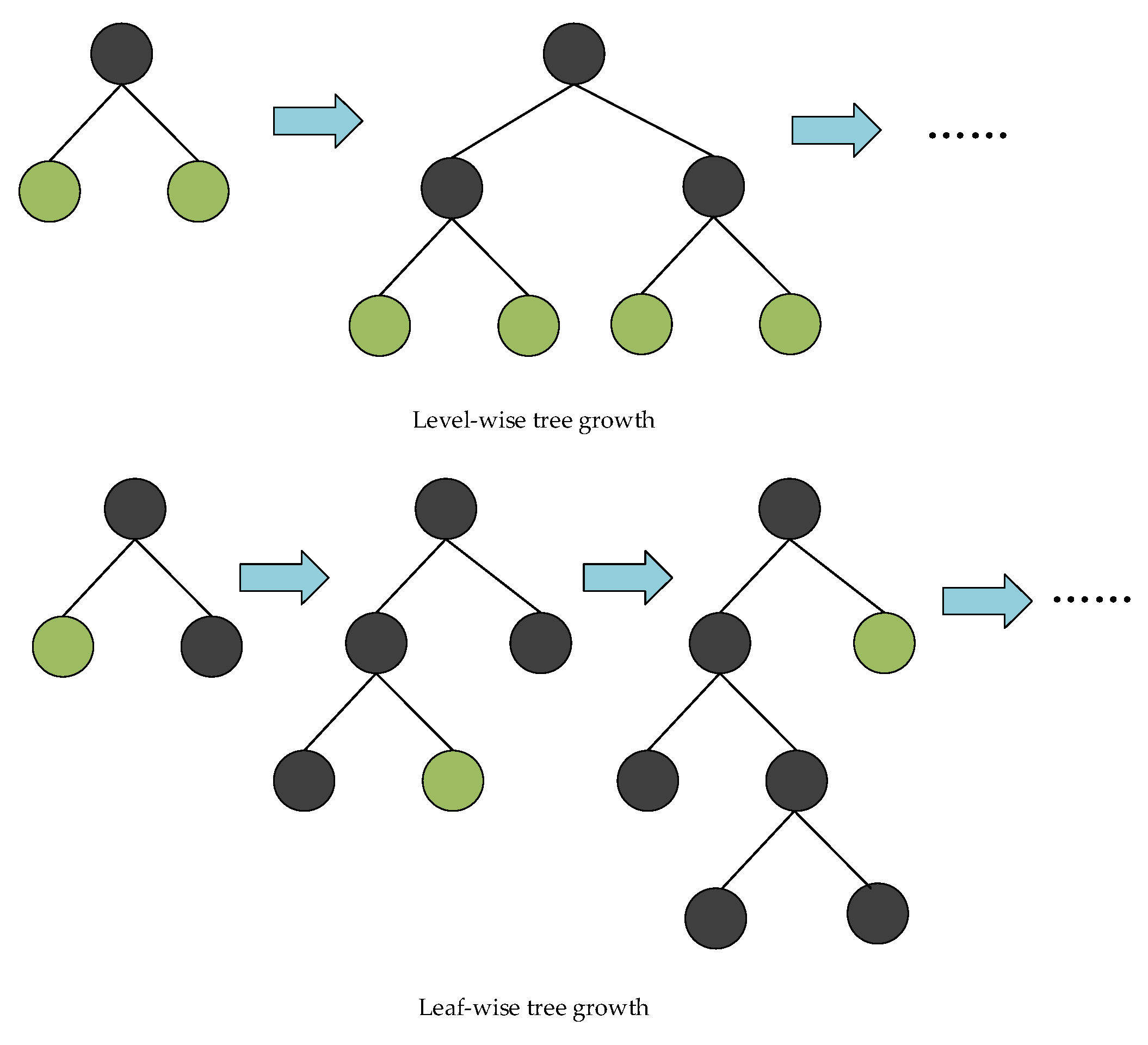
Figure 1. The strategy of tree growth in LightGBM.
Jmse 10 01150 g001
Figure 2. Schematic diagram of random forest prediction structure.
Jmse 10 01150 g002
Figure 3. The flowchart of the stacking model.
Jmse 10 01150 g003
Figure 4. The diurnal variation of hmax: (a) The changes on 1 February, 1 March, 1 April; (b) The changes on 1 May, 1 June, 1 July; (c) The changes on 1 August, 1 September, 1 October; (d) The changes on 1 November, 1 December, 1 January.
Jmse 10 01150 g004
Figure 5. The regression graph between several features and the target.
Jmse 10 01150 g005
Figure 6. Schematic diagram of stacking algorithm based on 5-fold cross-verification.
Jmse 10 01150 g006
Figure 7. The prediction performance of XGBoost: (a) The scatter plot between predicted value and true value; (b) The scatter plot between prediction residual and true value; (c) The histogram of z in the model.
Jmse 10 01150 g007
Figure 8. The prediction performance of LightGBM: (a) The scatter plot between predicted value and true value; (b) The scatter plot between prediction residual and true value; (c) The histogram of z in the model.
Jmse 10 01150 g008
Figure 9. The prediction performance of RF: (a) The scatter plot between predicted value and true value; (b) The scatter plot between prediction residual and true value; (c) The histogram of z in the model.
Jmse 10 01150 g009
Figure 10. The prediction performance of AdaBoost: (a) The scatter plot between predicted value and true value; (b) The scatter plot between prediction residual and true value; (c) The histogram of z in the model.
Jmse 10 01150 g010
Figure 11. The prediction performance of stacking: (a) The scatter plot between predicted value and true value; (b) The scatter plot between prediction residual and true value; (c) The histogram of z in the model.
Jmse 10 01150 g011
Figure 12. The prediction performance of improved stacking: (a) The scatter plot between predicted value and true value; (b) The scatter plot between prediction residual and true value; (c) The histogram of z in the model.
Jmse 10 01150 g012
Table 1. Explanations of abbreviated symbols.
SymbolIllustrationUnits
u10the horizontal speed of air moving toward the east, at a height of ten meters above the surface of the earthm/s
v10the horizontal speed of air moving toward the north, at a height of ten meters above the surface of the earthm/s
airMassthe mass of air per cubic meter over the oceanskg/m3
cdwwthe resistance that ocean waves exert on the atmospheredimensionless
vertVan estimate of the vertical velocity of updraughts generated by free convectionm/s
mpwwthe average time for two consecutive wave crests, on the surface of the sea generated by local winds, to pass through a fixed points
mslthe pressure (force per unit area) of the atmosphere at the surface of the earthPa
windthe horizontal speed of the “neutral wind”, at a height of ten meters above the surface of the earthm/s
sstthe temperature of seawater near the surfaceK
spthe pressure (force per unit area) of the atmosphere at the surface of land, sea, and inland waterPa
hmaxan estimate of the height of the expected highest individual wave within a 20 min windowm
Table 2. The statistics of individual features.
FeaturesMinimum ValueMaximum ValueMedian Value
u10 (m/s)−17.94011.734−3.174
v10 (m/s)−18.11112.1390.705
airMass (kg/m3)1.1321.2111.160
cdww (dimensionless)0.00060.0030.0011
vertV (m/s)0.00011.7340.713
mpww (s)1.5179.2983.476
msl (Pa)99,522.455102,522.813101,082.747
wind (m/s)2.00018.1416.621
sst (K)296.405304.136300.774
sp (Pa)99,522.562102,523.899101,083.687
hmax (m)0.72711.2632.253
Table 3. The nomenclature of the paper.
AbbreviationIllustration
XGBoostThe extreme gradient boosting
LightGBMThe light gradient boosting machine
RFThe random forest
AdaBoostThe adaptive boosting
LRThe linear regression
MAEThe mean absolute error
MSEThe mean squared error
R2The r2 score
Table 4. Model evaluations of different models on training and test sets.
DatasetsParametersXGBoostLightGBMRFAdaBoostStackingImproved Stacking
training setsMAE0.4460.4470.4450.4170.2840.281
MSE0.3720.3210.3440.2590.1540.150
R20.8950.9090.9020.9260.9560.957
test setsMAE0.4590.4640.4610.4330.2780.278
MSE0.3990.3590.3750.2850.1410.140
R20.8880.8990.8950.9200.9600.961
Table 5. The base model prediction performance.
ParametersXGBoostLightGBMRFAdaBoost
corr0.9640.9780.9470.962
std_resid0.5670.6000.6120.521
number of samples z > 334223612
Publisher’s Note: MDPI stays neutral with regard to jurisdictional claims in published maps and institutional affiliations.