Abstract
This article presents a model study of the dynamics of icebergs and surface floats in the Labrador Sea. The model was forced with data on the wind above the ocean surface, surface waves, and ocean currents. These data were obtained from the reanalysis of near-surface characteristics of the ocean and atmosphere for the year 2008. Icebergs and floats launched in an area north of the Labrador coast and to the east of Greenland generally move southeastward until they reach a boundary current “highway”. After that, they are carried by ocean currents into the central part of the subpolar North Atlantic. Simulations demonstrated that, for smaller icebergs, the primary balance is between the air and water drag, while for larger icebergs, it is between three forces: the air and water drag and the combined Coriolis and pressure forces. Floats, on the other hand, are driven mostly by the Ekman component of the surface velocity, while the geostrophic and Stokes components are less important. The significant variability in the motion of icebergs and floats is due to storms passing over the Labrador Sea, since these high-wind events introduce time-dependent dynamics.
1. Introduction
Icebergs of different shapes and sizes drifting past the shores of Newfoundland are a major tourist attraction, but they require our attention for other reasons as well. The fact that icebergs present danger to shipping, as well as to offshore oil platforms, is well known. Icebergs are indicators of climate change, to which the polar ocean is most sensitive; they can potentially affect local ocean environments and ecosystems. In the Labrador Sea, icebergs originate from the Labrador and Greenland glaciers and then travel around the sea, driven by the current, wind, and waves.
Calving of icebergs from terrestrial glaciers is a source of freshwater flux into the ocean with important implications for ocean climate. The mass loss of glaciers due to calving from Antarctica and Greenland is estimated to be about Gt/year [1,2]. The processes of the melting and erosion of icebergs along their paths influence the salinity in the ocean surface layer. Understanding the role of icebergs in the global freshwater budget requires a quantitative description of their dynamics and trajectories. The present study is motivated by the climate issues: Its goal is to contribute to the understanding of iceberg dynamics, particularly during storms passing over the Labrador Sea.
Iceberg velocities are normally computed using the momentum equation, which is driven by environmental forcing terms. The major forces are the air and water drag, the Coriolis force, and the pressure gradient force [3]. Although the formulation of the forces is straightforward, the problem is in the details of their parameterization. Perhaps the most important detail is the velocity field in the ocean surface layer. This field has to be provided with sufficiently high spatial and temporal resolution. The horizontal component of velocity should ideally be resolved up to the sub-mesoscale, which is not currently achievable. Sub-mesoscale motions include eddies, meanders, filaments, and fronts with spatial scales in the range between 1 and 100 km. Icebergs and floats are affected by these smaller-scale motions in the same way as they are affected by larger (mesoscale) motions. Thus, their effects on iceberg trajectories should either be resolved or parameterized, which is yet to be done. The vertical variation of velocity must also be accounted for because icebergs reach quite deep below the ocean surface. In the Arctic, smaller icebergs have keels that typically reach depths of 50 to 100 m; bigger icebergs can reach up to 400 m in depth [4]. Ocean currents, especially the Ekman and Stokes components, vary significantly in both magnitude and direction across the surface Ekman layer of a typical depth of 50 m. In the future, high-resolution satellite data might be available. In anticipation of this, we develop a model that can be “fed” by satellite altimetry data, as well as data on wind velocity and surface waves. Our model, however, goes beyond geostrophy and includes higher-order terms that are due to the unsteady and nonlinear character of the flow. In this paper, we study the response of icebergs to high-frequency hourly surface winds and eddy-resolving ocean currents. Wind forcing affects the velocity field via the Ekman velocity component while the waves contribute as the Stokes component; both components are depth dependent.
In addition to the momentum equation, an iceberg model requires equations that describe iceberg melting. Melting is due to turbulent heat exchange between icebergs and their environment, as well as due to erosion, which is caused by turbulent buoyant convection. An empiric melting model was developed by Bigg et al. [5] and used by Martin and Adcroft [2] and Wagner et al. [6]. As a result of melting, icebergs change their size and shape during their journey. The changes in an iceberg’s mass result in a shift in balance between the forces applied on the iceberg.
Recently, iceberg models were successfully coupled with general circulation models (GCMs) of oceans (e.g., [3,5,7,8,9]). The comparisons of real iceberg trajectories with model hindcasts showed that these models can perform reasonably well within a short time period of about one day. However, apart from general concepts of iceberg physics and thermodynamics, little is known about the dynamics of icebergs over long distances [10]. The main problems in the accurate prediction of iceberg trajectories in long-term simulations are due to uncertainties in the parameters of icebergs, such as their size and shape, and in the empirical parameters, as well as due to forcing by the ocean and wind. High-frequency wind variations can have a significant impact on icebergs’ motion. Gladstone et al. [11] simulated long-term iceberg trajectories by using atmospheric forcing from the European Center for Medium-Range Weather Forecasting (ECMWF) and adding 2.5 days of variations with amplitudes of 10 m/s to represent passing storms. In this work, we focus on the long-term computation of trajectories. Instead of studying particular individual cases, we launch clusters of identical icebergs and observe general patterns of their motion given the oceanic and atmospheric conditions in the Labrador Sea. The iceberg model is driven by the latest version of the ECMWF hourly reanalysis data (ERA5).
Sea ice and iceberg models have also been included in global climate models (e.g., [2,12,13,14,15,16,17]). It is also worth mentioning that GCMs have been used quite effectively to track other floats, such as plastic debris [18].
Surface drifters and profiling floats have become an integral part of observational oceanography [19]. Floats provide a “Lagrangian point of view” of the ocean dynamics, and they are important for understanding other floating objects, including debris, pollution, sea ice, and icebergs. In this article, we present a case study of ensemble simulations of surface floats and icebergs in the Labrador Sea with forcing data for the year 2008. We investigate which of the environmental forcing factors are more important in the dynamics of floats and icebergs. In particular, the roles of different components of surface velocity for surface floats are investigated. For icebergs, the relative importance of forcing terms, including form drag due to ocean currents and wind, is investigated; the components of the seawater velocity affect the dynamics of icebergs via these forcing terms.
The rest of this paper is organized as follows. In Section 2, we describe the equation of motion of an iceberg forced by ocean currents and wind. Section 2 also contains pertinent information about the dynamics of the upper ocean layer. In particular, geostrophic and ageostrophic components of the current velocity, including those due to wind stress and waves at the surface, are specified. Section 3 contains details on the remotely sensed environmental data used to run the model, as well as a description of the numerical algorithm of the model. Section 4 describes the computed iceberg trajectories, and Section 5 gives concluding remarks.
2. Theory
The dynamics of icebergs or smaller objects floating at the surface of water are controlled by currents and wind. Forcing terms in the momentum equation depend on the near-surface ocean and atmospheric characteristics that can be determined from remotely sensed observations of the ocean surface and the output of numerical reanalysis.
2.1. Iceberg Drift
The equation of motion of an iceberg can be written as
where M and are the mass and the horizontal velocity of the iceberg, respectively, f is the Coriolis parameter, is the vertical unit vector, is the force due to the pressure gradient in the water, and and are the water and air drag, respectively. The forcing terms on the right-hand side of (1) can be specified as follows. The horizontal pressure gradient, , is due to the variation of the sea surface height in the horizontal; it is the same pressure gradient that drives the ocean current [3,5]. The force on the iceberg is
where is the seawater density, is the sea surface height (SSH), and is the geostrophic velocity of the ocean current. Equation (2) shows that either SSH measured by a satellite altimeter or the geostrophic velocity can be used to compute . Moving the Coriolis term in the brackets to the right-hand side of (1) and combining it with , we obtain
Henceforth, we call this term the combined Coriolis and pressure gradient force. The water and air drag terms are given by usual quadratic drag equations:
where and are the velocities of the ocean current and air (wind), respectively, and are the drag coefficients, and and are the cross-sectional areas of the iceberg under and above the water, respectively. The drag coefficients depend on the form of an object; for simplicity, we take both of them as equal to unity, as for a cylinder. Note that we only consider quadratic (form) drag and do not take skin friction that occurs due to turbulent momentum transfer in the boundary layer around the iceberg into account.
Melting changes an iceberg’s aspect ratio and mass. In our simulations, we adopt an empiric melting model developed by [3] (see also [2,6]). The dominant processes that cause melting include (i) sidewall erosion due to surface waves , (ii) sidewall erosion due to buoyant convection , and (iii) basalt melt due to turbulent heat exchange at the base of an iceberg . These quantities give the rate of change in the linear dimensions of an iceberg and are parameterized as
and
where ms, , m sC, m sC, and m sC are the empirical coefficients, is the seawater temperature, and is the iceberg temperature, which is assumed to be fixed at = −4 C. The iceberg horizontal dimensions evolve as , while the vertical dimension evolves as [6].
2.2. Ocean Currents in the Surface Layer
To complete the iceberg drift model, we need to obtain the current velocity in the surface layer of the ocean. It is defined as a sum of the geostrophic and ageostrophic components , where , in turn, can be decomposed into a number of components such that
The first two terms on the RHS of (9) occur due to the unsteady and nonlinear character of the momentum equations of water and can be written as [20,21]
where J is the Jacobian operator (the determinant of the matrix of partial derivatives), which, in Cartesian geometry, is . The temporal derivative or tendency, , is calculated via the finite difference between two successive data fields in a sequence. Note that the ageostrophic components and are routinely computed in laboratory experiments with high-resolution altimetry [22,23,24,25,26,27].
The remaining two terms in (9) are the Ekman and Stokes components, respectively [28,29]. They account for the Ekman currents due to wind stress at the surface of the ocean, as well as the Stokes drift due to surface gravity waves. Classic Ekman surface-boundary-layer theory describes a wind-stress-induced current and its variation with depth such that
where is the characteristic depth of the Ekman layer, , is the effective vertical viscosity in the upper ocean, and is the wind stress. Note that cannot be measured directly by remote means, but it was shown to be related to the wind velocity , which can be obtained from satellite data. A useful approximation is , where all quantities are in SI units [29,30,31]. The last term in (9) accounts for the modification of the Ekman boundary layer by surface gravity waves and can be written as [28,32,33]
where is the Stokes drift given by [34]
where a is the wave amplitude, is the wavenumber vector, and is the wave frequency related to the wavenumber k via a dispersion relation for deep-water waves. The wave amplitude can be obtained from the significant wave height data, and . The direction and magnitude of the wave vector can be obtained from remotely sensed mean wave direction and period data; k is related to the wave period T via the dispersion relation such that .
3. Data and Methods
We present the results from a case study from the year 2008. Our computational domain includes the entire Labrador Sea and extends from N to N and from W to W (Figure 1). The forcing data (Figure 2) include ocean currents, wind velocity, and the characteristics of surface waves. The latter consist of the mean wave period T, mean wave direction , and the significant height of the combined waves and swells . The wind and surface wave characteristics were derived from the hourly ECMWF reanalysis (ERA5) [35] with a spatial resolution of . ERA5 is the fifth-generation ECMWF reanalysis [36], which has been extensively used in studies of the subpolar North Atlantic over the last few years [37,38]. The ERA5 surface atmospheric fields over the Labrador Sea were validated and compared with those obtained in other reanalyses in [39].
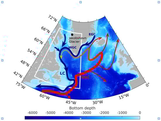
Figure 1.
Map of the computational domain and circulation in the subpolar North Atlantic. The arrows show major currents in the subpolar gyre, including the North Atlantic Current (NAC), the Eastern Greenland Current (EGC), the Western Greenland Current (WGC), and the Labrador Current (LC).

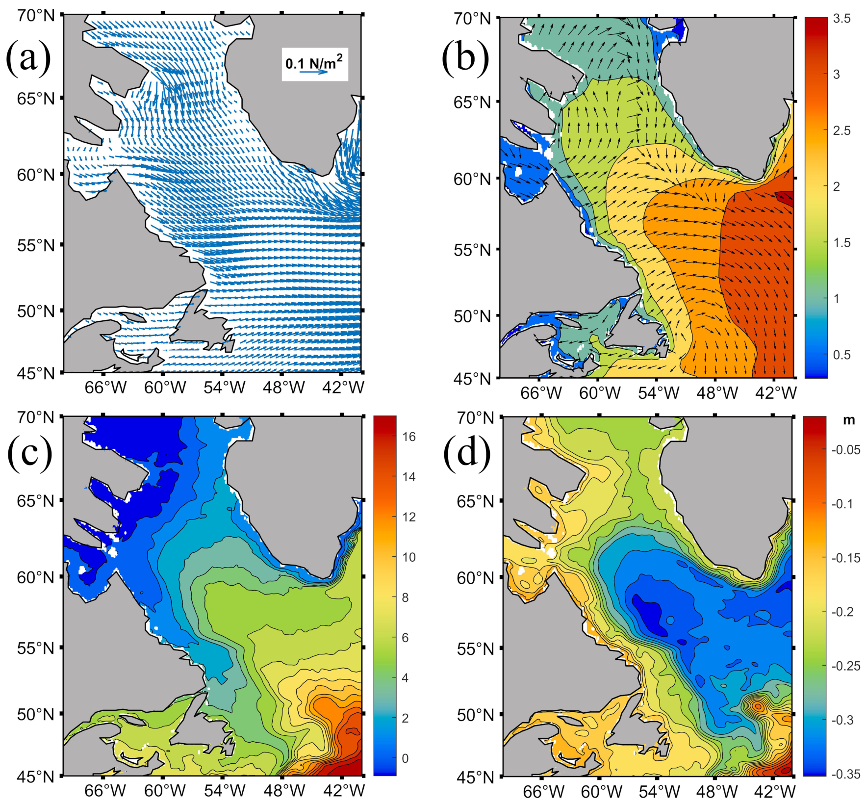
Figure 2.
Annual mean surface forcing used in the iceberg model due to: (a) surface wind stress; (b) direction and mean height of surface waves; (c) sea surface temperature (contour interval C); (d) sea surface height (contour interval 2 cm).
The ocean current, sea surface height, and sea surface temperature are from the MERCATOR Ocean International daily reanalysis provided by the Copernicus Programme (https://marine.copernicus.eu/, accessed 3 May 2022). All forcing data are spatially interpolated on a numerical grid.
In this study, we use the common assumption that the icebergs are of a cuboid shape of length L, width W, and height H. A typical ratio of an iceberg’s horizontal dimensions is [3]. In the vertical, the ratio of the subsurface depth or the draught of an iceberg to the total height can be easily found with
where kg/m is the density of the sea ice and kg/ is the seawater density. The above-water height (“freeboard” in nautical terminology) is, then, . Observations show that icebergs can be divided into several categories according to their size [11]. Here, we choose 8 categories of icebergs (Table 1), which correspond to categories 2–5 and 7–10 in [11].

Table 1.
The iceberg categories.
Surface floats and icebergs are considered to be Lagrangian particles, and their trajectories are computed through the integration of the kinematic equation
where is the position vector of a float or an iceberg. Floats are driven by the surface velocity such that the right-hand side (RHS) of (16) is simply the (Eulerian) velocity of the ocean current, . For icebergs, the RHS of (16) is the iceberg velocity, . The computation of float trajectories requires solving the single Equation (16). In contrast, the computation of iceberg trajectories involves solving several equations simultaneously, including the momentum Equation (1), Equations (6)–(8) describing melting and erosion, and the kinematic Equation (16). Numerical integration of these equations employs the fourth-order Runge–Kutta method.
Icebergs of each category are seeded over an area of offshore of the Jakobshavn glacier, which is a major source of icebergs in western Greenland [40]. The initial condition for iceberg velocities is obtained as a solution of the stationary version of Equation (1) with the forcing for 1:00 a.m. on 1 January 2008. The drag is calculated by averaging over the depth of the submerged part of the iceberg. Following [6], we assume that icebergs are oriented at a random angle relative to the wind and current. In this case, the long-term means of the vertical surface areas under and above the water are given by
4. Results
In this section, we describe the results of modeling of the trajectories of surface floats and icebergs for the year 2008, as well as the analysis of the relative importance of different components of the environmental forcing.
4.1. Surface Floats
Figure 3 shows the annual mean surface velocity and its components, namely, the quasigeostrophic, Ekman, and Stokes velocities. Here, the term “quasigeostrophic” is used for the sum of the geostrophic, nonlinear, and time-tendency components of the velocity. The standard deviation of the velocity components is shown in color. The quasigeostrophic velocity (Figure 3b) has its highest magnitude in the East and West Greenland currents and in the Labrador Current. These boundary currents are steered by the bottom topography and are intensified over the continental slope. They are strengthened by winds in the fall and winter seasons and decrease in the summer. The quasigeostrophic currents in the southern part of the region are influenced by the North Atlantic Current (NAC). This current is subject to high mesoscale eddy variability (Figure 3b). The annual mean Ekman currents have predominantly southward to southwestward directions (Figure 3c). The variations of the Ekman transport are most significant along the west coast of Greenland. The Stokes velocity has the smallest contribution to the annual mean surface currents (Figure 3d). It has a larger magnitude in the southeastern part of the region.
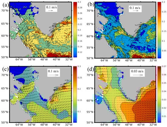
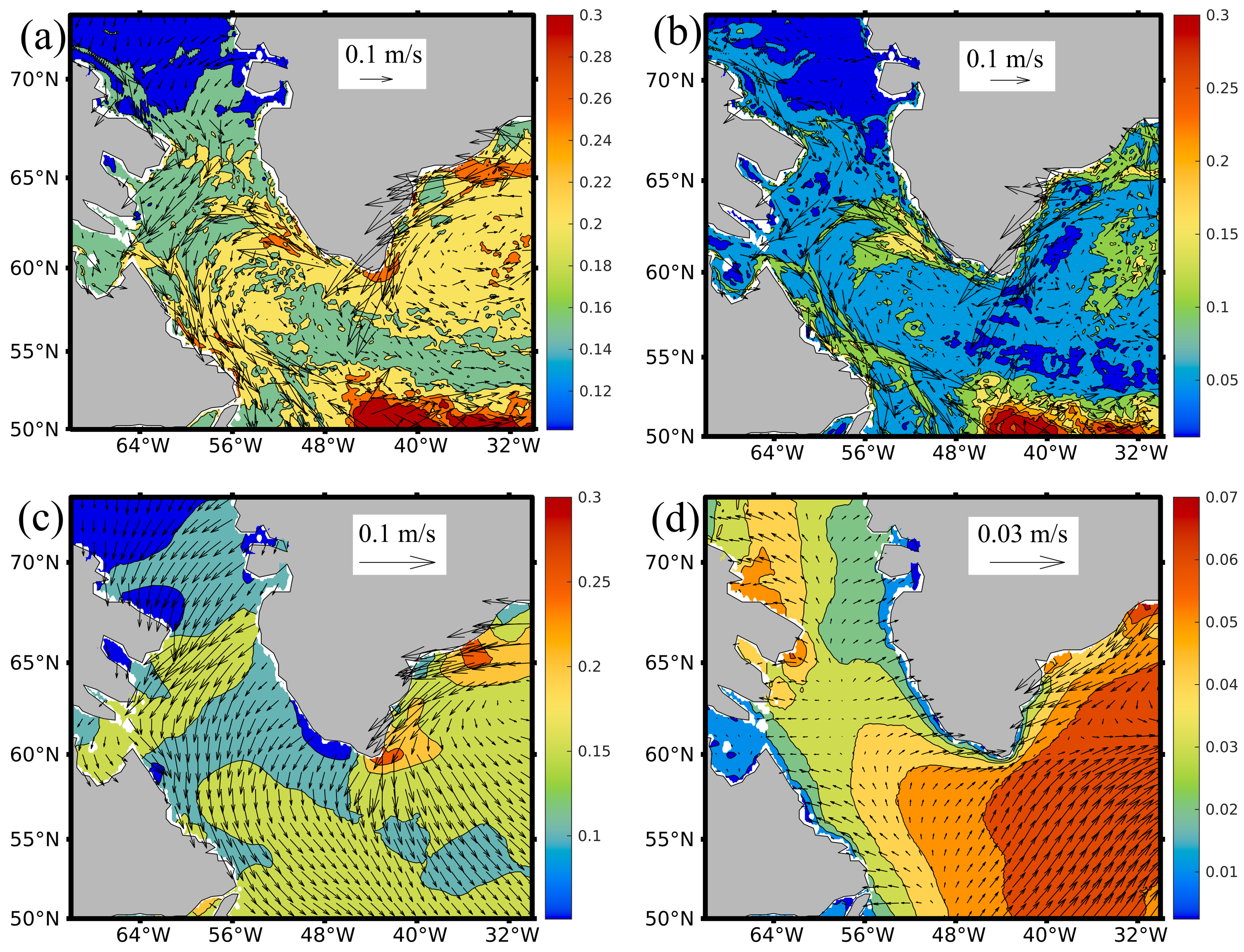
Figure 3.
Annual mean and contours of the standard deviation of (a) the ocean surface velocity (contour interval 0.05 cm/s), (b) the geostrophic velocity (contour interval 0.05 m/s), (c) the Ekman velocity (contour interval 0.05 m/s), and (d) the Stokes velocity (contour interval 0.01 m/s).
A comparison of the mean surface current (Figure 3a) with its individual components shows that it is quasigeostrophic to a certain degree in the boundary current along the coasts of Labrador and Greenland. In the northern part of the region and in the Baffin Strait, the Ekman component has a significant contribution (Figure 3c) to the mean and standard deviation of velocity. The time series show that the Ekman and Stokes components can intensify locally in areas of passing weather disturbances. These intensifications can affect the surface velocity locally for a relatively short period of time of several days.
In our model, floats were released in a domain on 1 January 2008. Figure 4a shows their trajectories for the time period of one year. The floats to the north of the Labrador coast and to the east of Greenland launched in cold waters (blue) tend to quickly converge towards the boundary current and then follow the boundary current “highway”. Indeed, the pattern of the surface Ekman velocity (Figure 3c) in these two regions is such that it carries the floats towards the boundary current, where they are picked up by the quasigeostrophic velocity.
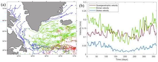
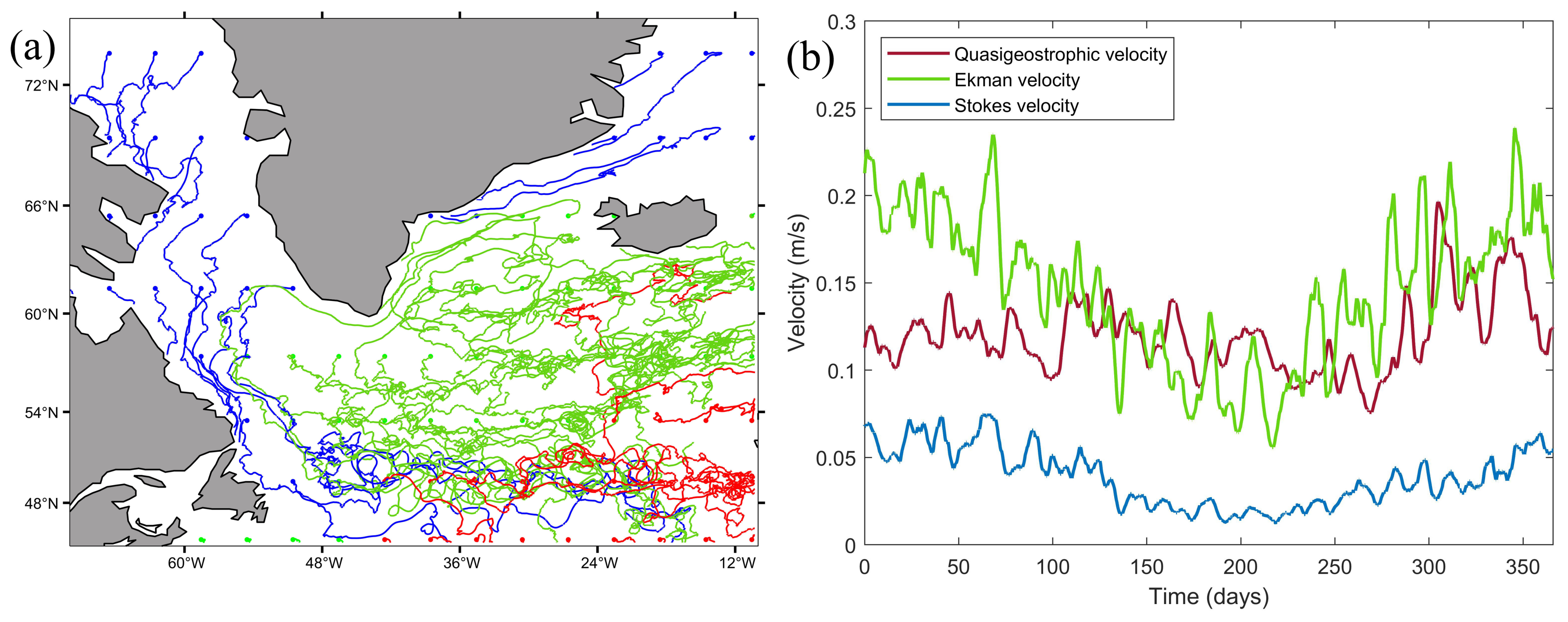
Figure 4.
Surface float trajectories (a) and velocity components (b). The trajectories are colored according to the annual mean sea surface temperature at the point of release: C (red), C (green), and C (blue). The quasigeostrophic (red line), Ekman (green line), and Stokes (blue line) components of velocity are averaged over the entire ensemble of floats.
In contrast, the floats released in the Atlantic Ocean south of Iceland (green) move quite chaotically and tend to linger in this area, which is characterized by strong mesoscale variability. In addition, the total surface velocity is relatively weak in the central part of this region (Figure 3a), which also contributes to the observed behavior of the floats.
The surface temperature shows that the most significant horizontal gradients are in the southern part of the region (see Figure 2). The Labrador Current brings cold freshwater along the coast of Newfoundland. The NAC transports warm salty waters of subtropical origin northeastward into the eastern subpolar North Atlantic. Most of the floats released in the warm southern part of the model region (red) move quickly along the NAC path. The baroclinic instability generates an intense mesoscale variability in the NAC (see Figure 3b). The related eddy-induced transport brings some of the floats released in the NAC into the central part of the Subpolar Gyre.
Figure 4b shows the components of the velocity averaged over the entire ensemble of floats. In addition, all three time series are low-pass filtered with a running 5-day window. The Ekman and Stokes components (green and blue, respectively) demonstrate clear seasonal variability with a larger magnitude in the winter and fall seasons (days 1–100 and 250–365). This is not surprising, since both of them are driven by wind. The unfiltered time series (not shown here) show high-frequency variations with a period of 2–3 days during strong storms. The magnitudes of these events are several times higher than the mean values. The seasonal cycle is less pronounced in the quasigeostrophic velocity component (red), which remains relatively flat during winter and spring, slightly decreases in the summer, and somewhat increases in the fall.
4.2. Icebergs
In contrast to floats, which are carried passively by surface currents, icebergs are directly exposed to wind above the surface of the water, as well as to currents in the deeper layers below the surface. As a result, their dynamics are more diverse. Different forcing terms in the momentum Equation (1) affect iceberg trajectories to different degrees. Smaller icebergs can be compared to a sailboat that is driven by wind and ocean currents. The dominant forces are from drags due to the motion of icebergs relative to the air and water [3]. Interestingly, air drag is a dominant force on a sail only when a boat is running downwind or in the so-called “broad reach” point of sail. When a boat is traveling at a right angle to the wind (beam reach), or even somewhat upwind (close-hauled), a lift force becomes dominant. This force occurs due to a shape of the sail which acts as an airfoil; the lift force is perpendicular to the wind. If an exact shape of an iceberg was known, one could compute the lift force in addition to the drag. However, this would require running a full hydrodynamic simulation of the flow around the iceberg, which is not practical. In addition, the lift is likely to be much smaller than the drag for most icebergs. For larger icebergs, the combined Coriolis and pressure gradient force becomes significant [6]. In our model, the forcing is derived from eddy-resolving ocean data and high-frequency 1-h surface forcing. This allows us to study how the balance of forces varies along iceberg trajectories for different categories of icebergs.
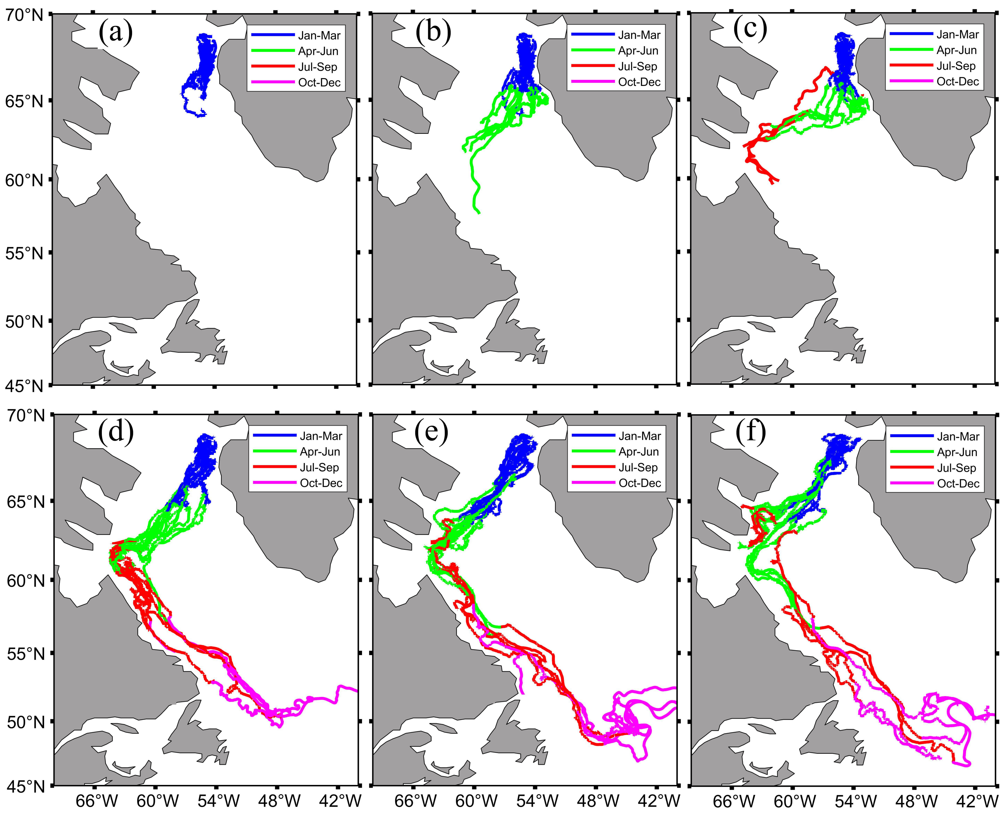
Figure 5 shows trajectories of 16 icebergs of each category (six categories out of the eight listed in Table 1). The icebergs are released in a small area offshore of the Jakobshavn Glacier. Not unlike the floats released in the same area, icebergs then follow the cyclonic circulation in the Labrador Sea, moving first southwestward towards the Hudson Strait and then following the direction of the boundary current along the coasts of Labrador and Newfoundland. However, there are essential differences as well. In contrast to floats, which are driven exclusively by surface current and leave the area of the northwestern part of the Labrador Sea fairly quickly, icebergs tend to linger there for a relatively long period of time of approximately 3 months. Smaller icebergs melt and never advance very far (Figure 5a). Larger icebergs, however, eventually make their way to the Labrador current and are carried out of the Labrador Sea to the open ocean.
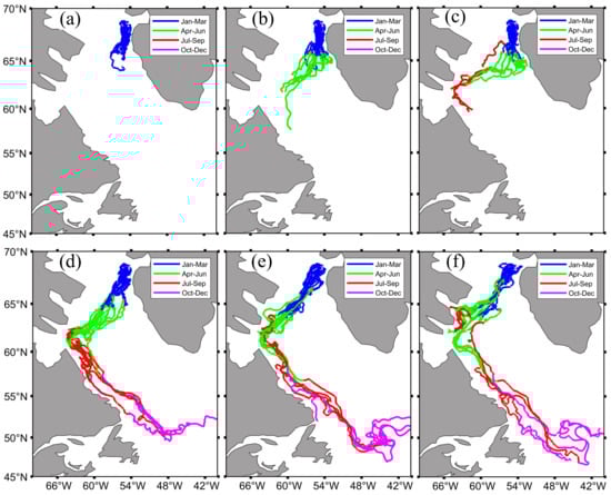
Figure 5.
Trajectories of icebergs of different masses: categories 3 (a), 4 (b), 5 (c), 7 (d), 9 (e), and 10 (f) (Table 1).
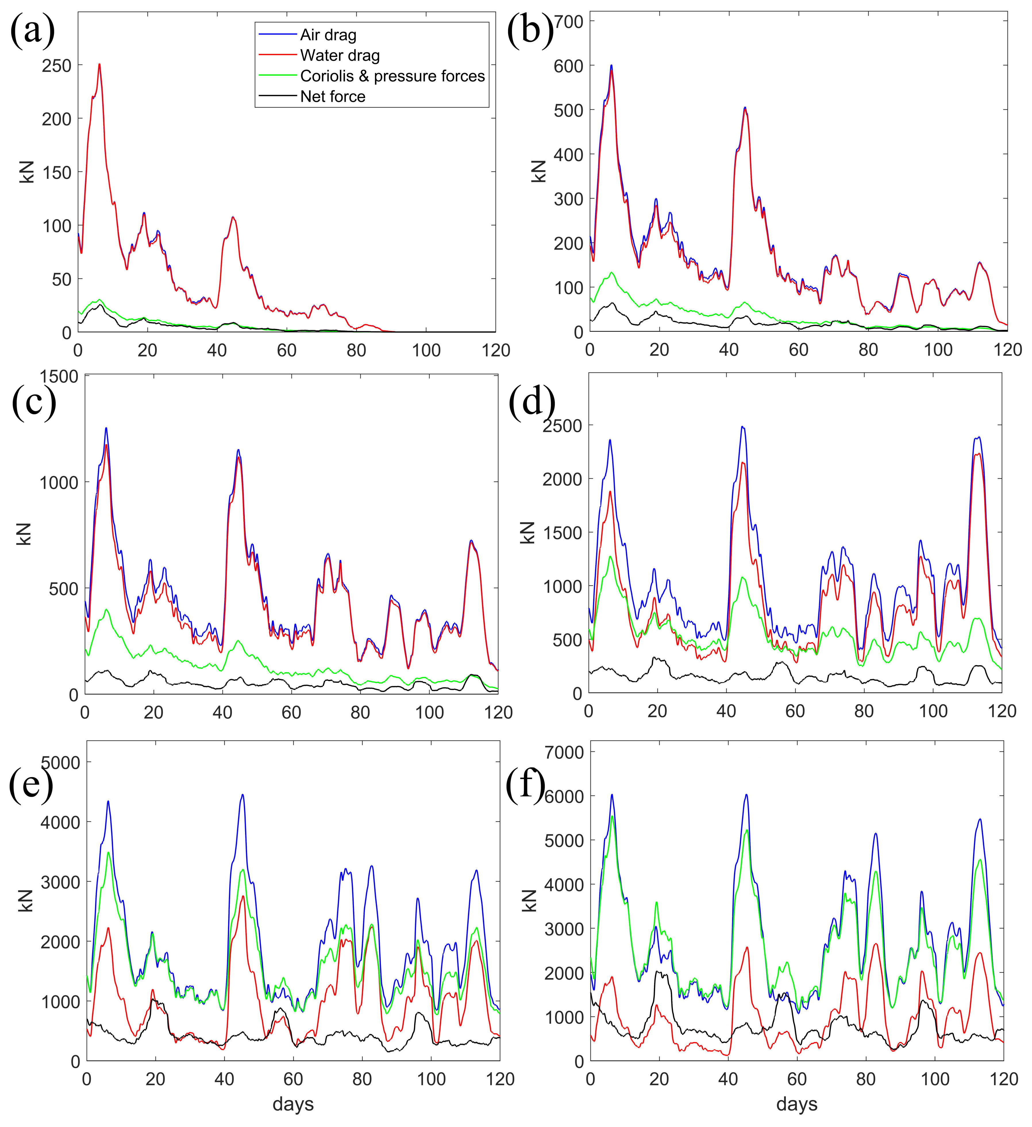
To further understand how the forces applied on icebergs vary during different weather events, in Figure 6, we plot their magnitude as a function of time for each cluster of icebergs. Only the first 120 days of the iceberg voyage are shown. Figure 6 shows that all forces exhibit variations related to weather disturbances passing over the region. Note that the time series in Figure 6 were filtered with a low-pass filter with a running 5-day window. The original data (not shown here) exhibit variability of an even higher frequency. During a storm, the air drag rapidly increases in magnitude over a period of several hours to one day. As a result, icebergs accelerate; the degree of acceleration can be deduced from the magnitude of the net force, which is shown as a black line in Figure 6. The increased iceberg velocity with respect to the water causes an increase in the water drag such that air and water drags become well balanced (“sailboat” behavior). Since the air and water drag cancel each other almost completely, the combined Coriolis and pressure gradient force is the one that determines the net force on the iceberg (also shown in Figure 6a).
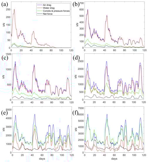
Figure 6.
The magnitude of forces applied on icebergs of different masses during the first 120 days of their journey: categories 3 (a), 4 (b), 5 (c), 7 (d), 9 (e), and 10 (f) (Table 1).
The almost identical variations in the air and water drag are exhibited by smaller icebergs, as shown in Figure 6a,b, while for larger icebergs (see Figure 6e,f), the combined Coriolis and pressure gradient force follows the air drag quite closely. The main reason that the balance of forces depends on the iceberg size is that the drag forces (4) and (5) and the combined Coriolis and pressure gradient force (3) scale differently with size. The drag forces are proportional to cross-sectional areas either under or above water, which both scale as the length squared. The combined Coriolis and pressure gradient force, , on the other hand, is proportional to the mass and, therefore, scales as the length cubed. Thus, becomes dominant for larger icebergs. Another consequence of the balance shift is that the water drag becomes relatively small. Since the water drag is proportional to the difference between the ocean current velocity and iceberg velocity, a small water drag indicates that these velocities are close. In other words, very large icebergs are mostly carried by ocean currents. Note, however, that the largest categories of icebergs are more typical for those observed in Antarctica, rather than in the Arctic.
Consider the evolution of forces during the single storm passing over the western North Atlantic on days 41–46. The vector diagrams in Figure 7 show the time series of forces for four icebergs of different masses. For the smaller icebergs (see Figure 7a,b), the air and water drag forces are in opposite directions but of the same amplitude; they are in almost perfect balance. The combined Coriolis and pressure gradient force is much smaller; together with the residual of the balanced stronger drag forces, it results in the total net force.
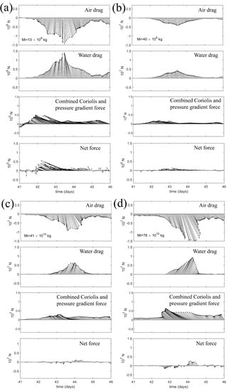
Figure 7.
Vector diagrams of forces for icebergs of different masses during a storm event: categories 4 (a), 5 (b), 9 (c), and 10 (d) (Table 1).
The forces are quite different for the larger icebergs in both direction and magnitude (Figure 7c,d). With the strongest wind on days 43–44, the air drag becomes very large. The water drag also increases significantly during this period, and, together with the combined Coriolis and pressure gradient force, it balances the air drag such that the resultant net force is relatively small compared to the individual components. It is also interesting to observe what happens when the winds are light (days 41–42) or moderate (days 45–46). The water drag becomes negligible, while the air drag and the combined Coriolis and pressure gradient force cancel each other almost exactly.
It is instructive to compare the direction of iceberg velocity with the wind and water velocities. Figure 8 shows vector diagrams of the velocity during the same days as those of the force diagrams in Figure 7. The velocity of the smaller icebergs is more closely aligned with the wind. The icebergs of categories 4 and 5 (shown in Figure 8a,b) deflect to the right of the wind by 20 and 24 , respectively. The magnitudes of iceberg velocity are approximately 1.4 and 1.0 of the wind speed for these two categories. These values are within the range of the observational estimates of 1.8 reported for icebergs in the Labrador Sea [7,41]. Note, however, that in dynamical models, the ratio of iceberg and wind velocities is sensitive to the values of the air and water drag coefficients. In operational models, these coefficients are routinely “tuned” to obtain a better agreement with observations. In our model, we did not attempt this because it was beyond our main focus. Larger icebergs drift at an angle of approximately 45 to the right of the wind in strong winds and at an angle of approximately 90 in light winds. The latter result is in agreement with the model from Wagner et al., where it occurred in the asymptotic case of large icebergs and light winds. Furthermore, comparing iceberg velocities with the surface velocity of seawater, one can see that they are quite different in both direction and magnitude for all icebergs. Since the surface velocity is the one carrying the surface floats, it is clear that icebergs drift differently.
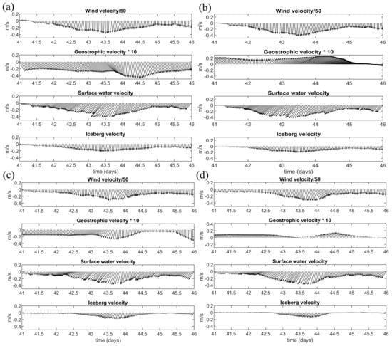
Figure 8.
Vector diagrams of air, water, and iceberg velocity for icebergs of different masses during a storm event: categories 4 (a), 5 (b), 9 (c), and 10 (d) (Table 1).
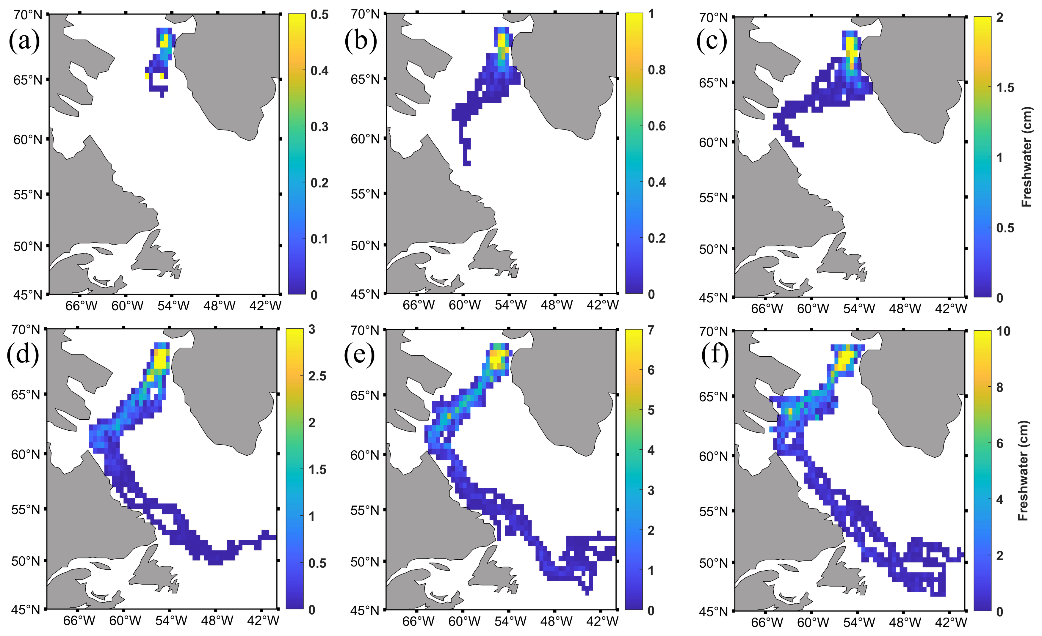
Icebergs melt during their journey, delivering cold freshwater to the environment. The amount of freshwater depends on how long an iceberg stays in a particular area, as well as on the control parameters in Equations (6)–(8). Perhaps the main parameter affecting the melting rate is the seawater temperature, . Figure 2c shows that seawater becomes warmer by approximately 2–3 C along a typical iceberg trajectory while following the boundary current from offshore of the Jakobshavn Glacier to the end of the Labrador coast. Beyond that, the seawater temperature rapidly increases in the eastern direction towards the warm waters of the NAC. Figure 9 shows the simulated amount of freshwater delivered by icebergs. This amount is averaged over an area of and is shown in cm. The pattern of melting is similar for all icebergs, although larger icebergs deliver more freshwater, as one might expect. The greatest amount of freshwater is deposited in the area west of Greenland, where icebergs spend more time. Similar melting patterns were reported in simulations by different authors [2,6].
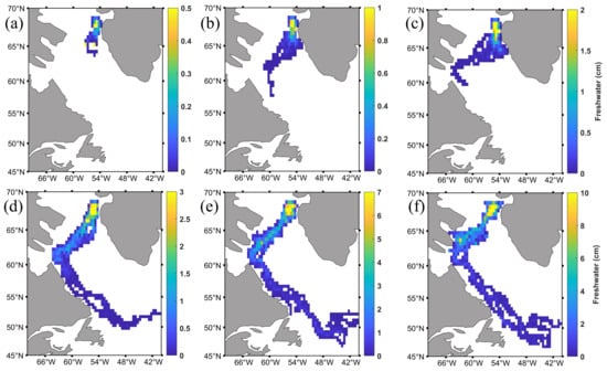
Figure 9.
Intensity of melting along the iceberg paths: categories 3 (a), 4 (b), 5 (c), 7 (d), 9 (e), and 10 (f) (Table 1).
5. Conclusions
In this paper, we described an idealized model of iceberg drift. The momentum equation of the model contains environmental forcing terms, including the air and water drag and the combined Coriolis and pressure gradient force. The model requires input data, which can be obtained through remote measurements. In particular, the seawater velocity can be computed using altimetry data, but it is not limited to geostrophy, as it includes higher-order terms due to nonlinearity and time tendency. Presently, we used the sea surface height from a reanalysis model, but in the future, high-resolution satellite altimetry data can be used directly. The measured characteristics of wind and surface waves allowed us to compute the Ekman and Stokes components of the velocity. Note that the latter two components are depth dependent; analytical equations were used to describe their vertical variation.
We simulated surface floats and iceberg trajectories in the Labrador Sea for the year 2008. Both floats and icebergs that start their journey west of the coast of Greenland converge into the Labrador current and are carried into the North Atlantic. Floats that are assumed to be passive Lagrangian tracers are carried by the surface velocity. The dominant component of the velocity is the Ekman component, especially in strong winds. The quasigeostrophic velocity, which is a sum of the geostrophic, nonlinear, and time-tendency components, is a close second.
Air and water drag and the combined Coriolis and pressure gradient force exerted on icebergs show high variability at synoptic time scales. This variability is driven by atmospheric disturbances passing over the Labrador Sea. Strong winds directly affect the air drag, while the water drag is affected via the Ekman component of the water velocity. While the duration of strong atmospheric disturbances is typically limited to a few days, the resulting forces on the iceberg can be significantly greater compared to their magnitude outside the storm periods.
Our present results show that the force balance and, hence, iceberg trajectories are significantly affected by temporal changes in their environment, such as those caused by weather events. In this work, the temporal resolution of input data was quite high, but the spatial resolution was not. The ocean data, although they were (mesoscale) eddy-resolving data, were still rather smooth on smaller (sub-meso) scales. When icebergs encounter sub-mesoscale oceanic motions, their trajectories are expected to deviate. Future simulations of iceberg trajectories should consider using sub-mesoscale ocean data with the goal of investigating the sensitivity of the trajectories to such “less smooth” forcing. These data can be provided by a high-resolution regional ocean model embedded in a global model.
Author Contributions
Conceptualization, Y.D.A. and E.D.; methodology, Y.D.A., E.D. and J.P.; writing—original draft preparation, J.P., E.D. and Y.D.A., data—acquisition J.P. and E.D., model—simulations and visualization, J.P. and E.D.; supervision, Y.D.A. and E.D. All authors have read and agreed to the published version of the manuscript.
Funding
J.P. and E.D. are supported by the Ocean Frontier Institute. Y.D.A. is supported by the Natural Sciences and Engineering Research Council of Canada.
Data Availability Statement
The data used to force the iceberg model in this study are existing data, which are openly available at https://resources.marine.copernicus.eu/ (accessed on 3 May 2022) and https://cds.climate.copernicus.eu/#!/home (accessed on 6 may, 2022), and they are cited in the reference section.
Acknowledgments
The authors are thankful to Stephanie Curnoe for proofreading the article.
Conflicts of Interest
The authors declare no conflict of interest.
References
- Hooke, R.L. Principles of Glacier Mechanics; Cambridge University Press: Cambridge, MA, USA, 2005. [Google Scholar]
- Martin, T.; Adcroft, A. Parameterizing the fresh-water flux from land ice to ocean with interactive icebergs in a coupled climate model. Ocean Model. 2010, 34, 111–124. [Google Scholar] [CrossRef]
- Bigg, G.R.; Wadley, M.R.; Stevens, D.P.; Johnson, J.A. Prediction of iceberg trajectories for the North Atlantic and Arctic oceans. Geophys. Res. Lett. 1996, 23, 3587–3590. [Google Scholar] [CrossRef] [Green Version]
- Schild, K.M.; Sutherland, D.A.; Elosegui, P.; Duncan, D. Measurements of Iceberg Melt Rates Using High-Resolution GPS and Iceberg Surface Scans. Geophys. Res. Lett. 2021, 48, e2020GL089765. [Google Scholar] [CrossRef]
- Bigg, G.R.; Wadley, M.R.; Stevens, D.P.; Johnson, J.A. Modelling the dynamics and thermodynamics of icebergs. Cold Reg. Sci. Technol. 1997, 26, 113–135. [Google Scholar] [CrossRef] [Green Version]
- Wagner, T.J.; Dell, R.W.; Eisenman, I. An analytical model of iceberg drift. J. Phys. Oceanogr. 2017, 47, 1605–1616. [Google Scholar] [CrossRef]
- Smith, S.D. Hindcasting iceberg drift using current profiles and winds. Cold Reg. Sci. Technol. 1993, 22, 33–45. [Google Scholar] [CrossRef]
- Kubat, I.; Sayed, M.; Savage, S.B.; Carrieres, T. An operational model of iceberg drift. Int. J. Offshore Polar Eng. 2005, 15, ISOPE-05-15-2-125. [Google Scholar]
- Turnbull, I.D.; Fournier, N.; Stolwijk, M.; Fosnaes, T.; McGonigal, D. Operational iceberg drift forecasting in Northwest Greenland. Cold Reg. Sci. Technol. 2015, 110, 1–18. [Google Scholar] [CrossRef]
- Marko, J.; Birch, J.; Wilson, M. A study of long-term satellite-tracked iceberg drifts in Baffin Bay and Davis Strait. Arctic 1982, 35, 234–240. [Google Scholar] [CrossRef] [Green Version]
- Gladstone, R.M.; Bigg, G.R.; Nicholls, K.W. Iceberg trajectory modeling and meltwater injection in the Southern Ocean. J. Geophys. Res. Oceans 2001, 106, 19903–19915. [Google Scholar] [CrossRef] [Green Version]
- Hunke, E.C.; Comeau, D. Sea ice and iceberg dynamic interaction. J. Geophys. Res. Oceans 2011, 116. [Google Scholar] [CrossRef] [Green Version]
- Losch, M.; Menemenlis, D.; Campin, J.M.; Heimbach, P.; Hill, C. On the formulation of sea-ice models. Part 1: Effects of different solver implementations and parameterizations. Ocean Model. 2010, 33, 129–144. [Google Scholar] [CrossRef] [Green Version]
- Hill, J.C.; Condron, A. Subtropical iceberg scours and melt water routing in the deglacial western North Atlantic. Nat. Geosci. 2014, 7, 806–810. [Google Scholar] [CrossRef]
- Jongma, J.I.; Driesschaert, E.; Fichefet, T.; Goosse, H.; Renssen, H. The effect of dynamic-thermodynamic icebergs on the Southern Ocean climate in a three-dimensional model. Ocean Model. 2009, 26, 104–113. [Google Scholar] [CrossRef]
- Bügelmayer, M.; Roche, D.M.; Renssen, H. How do icebergs affect the Greenland ice sheet under pre-industrial conditions?—A model study with a fully coupled ice-sheet–climate model. Cryosphere 2015, 9, 821–835. [Google Scholar] [CrossRef] [Green Version]
- Fitzmaurice, A. Parameterizing the Melting of Icebergs in Global Climate Models. Ph.D. Thesis, Princeton University, Princeton, NJ, USA, 2018. [Google Scholar]
- Maximenko, N.; Hafner, J.; Kamachi, M.; MacFadyen, A. Numerical simulations of debris drift from the Great Japan Tsunami of 2011 and their verification with observational reports. Mar. Pollut. Bull. 2018, 132, 5–25. [Google Scholar] [CrossRef]
- Roemmich, D.; Johnson, G.; Riser, S.; Davis, R.; Gilson, J.; Owens, W.; Garzoli, S.; Schmid, C.; Ignaszewski, M. The Argo Program: Observing the global ocean with profiling floats. Oceanography 2009, 22, 34–43. [Google Scholar] [CrossRef] [Green Version]
- Cushman-Roisin, B.; Chassignet, E.P.; Tang, B. Westward motion of mesoscale eddies. J. Phys. Oceanogr. 1990, 20, 758–768. [Google Scholar] [CrossRef]
- Afanasyev, Y.D. Altimetry in a GFD laboratory and flows on the polar β-plane. In Modelling Atmospheric and Oceanic Flows: Insights from Laboratory Experiments and Numerical Simulations; von Larcher, T., Williams, P., Eds.; AGU Wiley: Hoboken, NJ, USA, 2015; Chapter 5; pp. 101–117. [Google Scholar]
- Afanasyev, Y.D.; O’Leary, S.; Rhines, P.B.; Lindahl, E.G. On the origin of jets in the ocean. Geoph. Astroph. Fluid Dyn. 2012, 106, 113–137. [Google Scholar] [CrossRef]
- Afanasyev, Y.D.; Rhines, P.B.; Lindahl, E.G. Velocity and potential vorticity fields measured by altimetric imaging velocimetry in the rotating fluid. Exp. Fluids 2009, 47, 913–926. [Google Scholar] [CrossRef]
- Zhang, Y.; Afanasyev, Y. Beta-plane turbulence: Experiments with altimetry. Phys. Fluids 2014, 26, 026602. [Google Scholar] [CrossRef] [Green Version]
- Matulka, A.M.; Zhang, Y.; Afanasyev, Y.D. Complex environmental β-plane turbulence: Laboratory experiments with altimetric imaging velocimetry. Nonlinear Process. Geophys. 2016, 23, 21–29. [Google Scholar] [CrossRef] [Green Version]
- Zhang, Y.; Afanasyev, Y. Baroclinic turbulence on the polar beta-plane in the rotating tank: Down to submesoscale. Ocean Model. 2016, 107, 151–160. [Google Scholar] [CrossRef]
- Afanasyev, Y.D. Turbulence, Rossby waves and zonal jets on the polar β-plane: Experiments with laboratory altimetry. In Zonal Jets: Phenomenology, Genesis, and Physics; Galperin, B., Read, P.L., Eds.; Cambridge University Press: New York, NY, USA, 2019; Chapter 8; pp. 152–166. [Google Scholar]
- Wu, K.; Liu, B. Stokes drift–induced and direct wind energy inputs into the Ekman layer within the Antarctic Circumpolar Current. J. Geophys. Res. Oceans 2008, 113. [Google Scholar] [CrossRef] [Green Version]
- Hui, Z.; Xu, Y. The impact of wave-induced Coriolis-Stokes forcing on satellite-derived ocean surface currents. J. Geophys. Res. Oceans 2016, 121, 410–426. [Google Scholar] [CrossRef] [Green Version]
- Ekman, V.W. On the Influence of the Earth’s Rotation on Ocean-Currents; Arch. Math. Astron. Phys. 1905, 2, 1–52. [Google Scholar]
- Santiago-Mandujano, F.; Firing, E. Mixed-layer shear generated by wind stress in the central equatorial Pacific. J. Phys. Oceanogr. 1990, 20, 1576–1582. [Google Scholar] [CrossRef] [Green Version]
- Liu, B.; Wu, K.; Guan, C. Global estimates of wind energy input to subinertial motions in the Ekman-Stokes layer. J. Oceanogr. 2007, 63, 457–466. [Google Scholar] [CrossRef]
- Polton, J.A.; Lewis, D.M.; Belcher, S.E. The role of wave-induced Coriolis–Stokes forcing on the wind-driven mixed layer. J. Phys. Oceanogr. 2005, 35, 444–457. [Google Scholar] [CrossRef]
- Philipps, O.M. The Dynamics of the Upper Ocean; Cambrige University Press: Cambrige, MA, USA, 1977. [Google Scholar]
- Hersbach, H.; Bell, B.; Berrisford, P.; Biavati, G.; Horányi, A.; Muñoz Sabater, J.; Nicolas, J.; Peubey, C.; Radu, R.; Rozum, I.; et al. ERA5 Hourly Data on Single Levels from 1959 to Present. Copernicus Climate Change Service. Climate Data Store (CDS). 2018. Available online: https://cds.climate.copernicus.eu/#!/home (accessed on 6 May 2022).
- Hersbach, H.; Berrisford, B.B.; Hirahara, S.; Horányi, A.; Muñoz-Sabater, J.; Peubey, J.N.; Radu, R.; Schepers, D.; Simmons, A.; Soci, C.; et al. The ERA5 global reanalysis. Q. J. R. Meteorol. Soc. 2020, 146, 1999–2049. [Google Scholar] [CrossRef]
- Li, F.; Lozier, M.S.; Bacon, S.; Bower, A.S.; Cunningham, S.A.; de Jong, M.F.; deYoung, B.; Fraser, N.; Fried, N.; Han, G.; et al. Subpolar North Atlantic western boundary density anomalies and the Meridional Overturning Circulation. Nat. Commun. 2021, 12, 3002. [Google Scholar] [CrossRef] [PubMed]
- New, A.L.; Smeed, D.A.; Czaja, A.; Blaker, A.T.; Mecking, J.V.; Mathews, J.P.; Sanchez-Franks, A. Labrador Slope Water connects the subarctic with the Gulf Stream. Environ. Res. Lett. 2021, 16, 084019. [Google Scholar] [CrossRef]
- Pennelly, C.; Myers, P.G. Impact of different atmospheric forcing sets on modeling Labrador Sea Water production. J. Geophys. Res. Oceans 2021, 126, e2020JC016452. [Google Scholar] [CrossRef]
- Holland, D.M.; Thomas, R.H.; De Young, B.; Ribergaard, M.H.; Lyberth, B. Acceleration of Jakobshavn Isbræ triggered by warm subsurface ocean waters. Nat. Geosci. 2008, 1, 659–664. [Google Scholar] [CrossRef]
- Garrett, C.; Middleton, J.; Hazen, M.; Majaess, F. Tidal Currents and Eddy Statistics from Iceberg Trajectories off Labrador. Science 1985, 227, 1333–1335. [Google Scholar] [CrossRef]


Publisher’s Note: MDPI stays neutral with regard to jurisdictional claims in published maps and institutional affiliations. |
© 2022 by the authors. Licensee MDPI, Basel, Switzerland. This article is an open access article distributed under the terms and conditions of the Creative Commons Attribution (CC BY) license (https://creativecommons.org/licenses/by/4.0/).