ALOS-Based USV Path-Following Control with Obstacle Avoidance Strategy

Abstract

Path following and obstacle avoidances are used in heading control and path replanning for unmanned surface vessels (USVs), which have attracted the interest of many researchers over the years. This paper investigates the path-following and obstacle avoidance problems for USVs. First, on the basis of the current position and desired path, an adaptive line-of-sight (ALOS) algorithm is used to obtain the desired heading angle, and the sideslip angle compensation is considered. Then, to ensure that the USV follows the desired path. Model predictive control (MPC) is used to reduce the lateral error. The event-triggered mechanism (ETM) strategy is utilized to reduce the computational cost of MPC. Moreover, to obtain accurate state quantities in real time, a linear extended state observer (LESO) is used to counteract the effects of external disturbances and the nonlinear term of the model. Furthermore, an improved obstacle avoidance algorithm based on the geometric relationship is proposed. This method can better ensure USV navigation safety and reduce consumption and computation. Lastly, multiple simulation experiments illustrate that the algorithm improves the path-following capability and security and ensures smooth input changes by setting input constraints. Therefore, the designed controller has better feasibility and robustness.

1. Introduction

In recent years, many aspects of unmanned surface vessel (USV) studies have been challenging [1], such as USV navigation technology, USV guidance technology, USV control technology, and navigation and control for multiple USVs. USV guidance technology can be further divided into path planning and path replanning. Among these problems, expected path following and obstacle avoidance are two important topics in USV path planning and path replanning problems [2,3,4]. In [5], a novel path planning method was proposed. This method calculates the feasible path on the basis of the current environmental information, considering energy consumption. In [6], a path planning algorithm that extends the already existing $A^{*}$ approach was investigated. This approach solves path planning in the USV navigation environment by restricting the optimal path points using the boundary of a circle as a safety condition. In [7], a predicted trajectory approach was proposed. The optimal path selection for this approach was based on length, safety, and smoothness. Furthermore, all dynamic constraints were taken into account to further improve the control performance. The authors of [8] proposed an improved ant colony optimization/artificial potential field. This method was used to search for globally optimal paths in the grid map. Compared to the four methods above, the path generated by two adjacent points is simple to implement, reducing the amount of computation and improving the real-time performance.

To ensure that the USV follows the desired path, the line-of-sight (LOS) navigation algorithm is proposed to convert the path following into reducing the lateral error between the USV and the desired path [9]. However, since LOS lacks sensitivity to lateral error variations, an adaptive line-of-sight (ALOS) algorithm that adapts to error variations is applied to path following [10]. Furthermore, many control methods have been investigated to make the USV follow the desired path.

In [11], a proportional–integral–derivative-based controller was designed to generate commanded rudder deflections. In [12], the backstepping method was designed. In [13], suitable slip modes were designed to ensure system stability, which ensured that the surge and heading velocities could track the desired velocities separately. In the actual operation of the USV, the input, output, and state quantities of the entire system may be limited, which poses a challenge for the design of the controller. The methods mentioned above do not handle the limitation problem very smoothly. In contrast, model predictive control (MPC) is able to better handle the limitation in the USV heading process. In [14], a robust H-infinity-type state feedback model predictive control was proposed. This method was used to control the roll/yaw speeds of a ship while sailing while considering the effect of input limitations to improve the control performance. In [15], nonlinear MPC was used to handle the input limitation of USV. However, the high computational cost of MPC leads to limitations in its practical applications. In [16], a dynamic event-triggered control scheme was proposed. This approach was used to reduce the energy consumption from the controller to the actuator while designing dynamic parameters to improve the control performance according to dynamic conditions. To avoid the high computational costs and improve the practical application of MPC, an event-triggered mechanism (ETM) strategy that sets the maximum value of the measurement state error to design the trigger condition was proposed [17]. This method can effectively reduce the computational cost of MPC to ensure the system’s stability and simple structure.

USV is subject to external uncertainties, nonlinear dynamics, and state unpredictability during navigation [18]. The presence of these disturbances can affect the control performance of the controller. Ignoring these effects will lead to poorer control and increase the danger of navigation. The MPC controller depends heavily on the accuracy of the established USV model. To improve control performance, measures are needed to design the controller to resist disturbances, nonlinearities, and unpredictable effects. There are many results in the design of a research observer. In [19], a time-delayed extended state observer (ESO) was designed. The event-triggered ESO based on a reduced-order ESO was designed to estimate the position and velocity. Eventually, the better performance of the event-triggered ESO was confirmed through comparative simulation experiments. Previous work [20] proposed a trajectory tracking controller based on the homogeneous nonlinear extended state observer (HNESO) and the dynamic surface control. Compared with the conventional dynamics surface control, nonlinear model predictive, and adaptive sliding mode control (SMC) for multiple simulation experiments, the proposed algorithm in [20] performed better against interference. HNESO improves the estimation accuracy but undoubtedly increases the system model complexity and computational consumption. In addition, another problem of USV control obstacle avoidance is also considered during path following. USV obstacle avoidance research is also a popular current research direction. In [21], a dynamic navigation ship domain was proposed, which was used to achieve obstacle avoidance by inferring the collision risk in time on the basis of obstacle information and then planning the local path. In [22], an inland-ship collision avoidance decision system is proposed. This approach was used to solve the inland-ship collision avoidance problem. A sensor measurement-based obstacle avoidance law was proposed in [23], which could avoid unknown obstacles. However, the sensors may be more susceptible to noise interference. Previous work [23] proposed that the algorithm requires real-time reception of the sensor’s signal during obstacle avoidance, which may bring excessive energy consumption and reduce the real-time performance, as well as a slightly lower safety margin in obstacle avoidance path planning.

Considering the abovementioned issues and the existing works, this paper focuses on the following elements:

• To reduce the lateral error throughout the process, by changing the sight distance, the ALOS algorithm is used to make the USV follow the desired path. In order to consider the influence of the current on navigation, the ALOS algorithm is also designed with sideslip angle compensation to control the USV better to follow the desired path.
• The control methods mentioned above, such as PID and SMC, lack control of the input and states, making the input change sharply and increasing energy consumption and rudder wear. MPC has the advantages of better solving constraints and limitations due to the structure of the rudder. Therefore, the advantages of MPC are taken to solve the actual USV path following and construction constraints. The ETM strategy is used to reduce the computational effort of MPC to improve real-time performance.
• In the actual navigation environment, there are inevitably many unknown disturbances. In this paper, the effects of unknown disturbances and nonlinear terms are estimated in real time by a linear extended state observer (LESO) to improve the system’s control performance.
• The obstacle avoidance algorithm in [23] has problems in the face of known obstacles, such as the sensors being susceptible to noise, and it is computationally intensive because it achieves real-time detection. Therefore, on the basis of [23], a new obstacle avoidance algorithm for known obstacles is proposed. This algorithm does not require sensors to detect the edge of the obstacle in real time but only needs to use the location and obstacle information to achieve obstacle avoidance, which significantly reduces the amount of computation and the impact of environmental interference. An allowance is also added to ensure the safety of the USV obstacle avoidance process.

Section 2 presents the USV control model used in this paper, and, in Section 3, the controller design of the whole system is presented. Section 4 provides proof of the system stability. The proposed algorithm is subjected to multiple sets of comparative simulation experiments as shown in Section 5. Section 6 presents the conclusions and future research directions of this paper.

2. Mathematical Model

From a rigorous analysis, the USV model should be built using six degrees of freedom (DOFs), which is accurate but very difficult for practical control of the USV. Inspired by [24], different kinds of DOF models applied to other targets have been conveyed and confirmed. For example, a USV model with three DOFs is used to study the tracking of curved paths, and this model can be used to ensure the monitoring of velocities and not only for directions. It should be stated here that the USV studied in this paper lacks control of the sway velocity, but a propeller is equipped to keep the surge velocity constant, and a rudder is used to control the yaw of the USV. This paper applies a previously proposed model to accomplish the desired path following and obstacle avoidance. Thus, a one-DOF USV model is used to solve the objects mentioned above.

The second-order Nomoto model was studied in [25], which is as follows:

$$T_1{T}_2\ddot{r}+\left(T_1+T_2\right)\dot{r}+r=K\left(T_3\dot{\delta }+\delta \right),$$

(1)

where $r$ is the angular velocity of yaw, $K$, $T_1$, $T_2$, and $T_3$ are the parameters that affect USV rudder to heading control, and $\delta$ is the rudder angle. However, the Nomoto model (Equation (1)) has some problems, as illustrated by [26], which were corrected by the nonlinear item of $r$ proposed in [27]. Therefore, the Nomoto model (Equation (1)) can be written as

$$T_1{T}_2\ddot{r}+\left(T_1+T_2\right)\dot{r}+r+\alpha r^3=K\left(T_3\dot{\delta }+\delta \right).$$

(2)

A servo system controls the rudder angle of the USV with a time delay rather than directly acting on the actual system, which was modeled by [28,29], i.e., $\dot{\delta }=\left(K_{1}U-\delta \right)/T_4$, and it was also taken into account. Therefore, Equation (2) can be written as

$$T_1{T}_2\stackrel{⃛}{\psi }+\left(T_1+T_2\right)\ddot{\psi }+\dot{\psi }+\alpha {\dot{\psi }}^3=K\left(\frac{T_3\left(K_{1}U-\delta \right)}{T_4}+\delta \right),$$

(3)

where $K_1$ and $T_4$ are the parameters representing the gain and response time of the rudder servo system, respectively. If $U$ is the input variable, and $\psi$ is the output variable, the heading angle can be determined by $\dot{\psi }=r$. $\alpha$ is the coefficient of the nonlinear term. A coordinate transformation adding the nonlinear item and unknown disturbance is defined as follows:

$$\dot{x}=f\left(x,U\right)=\left[\begin{array}{l}{x}_2\\ x_3\\ h\left(x,U\right)+d\\ \frac{K_{1}U-x_4}{T_4}\end{array}\right],$$

(4)

where $x$ is the system states defined by $x=\left[\begin{array}{cccc}{x}_1& x_2& x_3& x_4\end{array}\right]=\left[\begin{array}{cccc}\psi & r& \dot{r}& \delta \end{array}\right]$, and $d$ is the system interference with the nonlinear item and unknown disturbance. The $h(x,U)$ derived by Equation (3) without the nonlinear item is expressed as

$$h\left(x,U\right)=\frac{1}{T_1{T}_2}\left[-{\left(T_1+T\right)}_2{x}_3-x_2+K{x}_4+\frac{K{T}_3}{T_4}\left(K_{1}U-x_4\right)\right].$$

(5)

3. Design of a Feasible System Control Strategy

Strategies can be decomposed into three fundamental subsystems: ALOS, MPC controller with ETM strategy, and LESO. ALOS is used to provide the right heading angle for the MPC. The MPC controller with the ETM strategy is used to reduce the error between the current heading angle of the system and the desired heading angle provided by ALOS. LESO is used to estimate the current actual state of the system. The block diagram of the whole system is shown in Figure 1.

3.1. Assumptions

In this paper, in order to improve the rigor and simplify the construction of the USV path-following model, the following assumptions are made:

• The velocities of USV in the sway direction and surge direction are constants, and the drift angle is also a constant.
• The shape of the obstacle and the safe region are circular. The information relative to USV frame of obstacle is available, including the position and radius of the circle.

3.2. The ALOS Guidance Strategy

When the desired path and heading angle are known, a USV located in any position to follow the path was first studied by Fossen in [7]. Furthermore, the LOS algorithm was introduced to convert the path-following problem to reduce the lateral error between the current position and the desired path. Meanwhile, the error revealed in the form of a lateral error can be calculated from the look-ahead distance and the difference $\tilde{\psi }=\psi -{\psi }_d$, as illustrated in Figure 2.

In Figure 2, $\Delta$ is the variable look-ahead distance as $e$ and the lateral error change. $u,v$ represent the surge velocity and sway velocity, respectively. $P_k$ is the predetermined current waypoint, and the next waypoint is $P_{k+1}$. $\beta$ is generated by the disturbance in the sway direction. As the lateral error increases, the look-ahead distance decreases correspondingly, guaranteeing efficient convergence to the path. However, as the traditional LOS algorithm is short of the look-ahead distance varying with the lateral error, inspired by [8], an adaptive LOS algorithm with the varying look-ahead distance is used, defined as follows

$$\Delta =\left({\Delta }_{max}-{\Delta }_{min}\right)exp^\left(-\frac{e^2}{u}\right),$$

(6)

where ${\Delta }_{max}$, ${\Delta }_{min}$ are the maximum and minimum boundary values of the look-ahead distance, respectively.

As a matter of fact, with the flow rate of water disturbance, it is evident that the course angle consists of the heading angle with the drift angle compensation generated by the disturbance in the sway direction. According to assumption 1, inspired by [30], the desired course angle ${\psi }_d$ with drift angle compensation and the latter error is as follows:

$${\psi }_d={\psi }_r-{\tan }^{-1}\left(\frac{e}{\Delta }\right)+{\tan }^{-1}\left(\frac{v}{u}\right),$$

(7)

where the ${\psi }_r$ is the course angle of desired path, and $\mathrm{v}$ is the sway velocity.

The derivative of the latter error is defined by Equation (8).

$$\dot{e}=u\sin \left(\psi -{\psi }_r\right)-v\cos \left(\psi -{\psi }_r\right).$$

(8)

From Equation (8), when the course angle tracks the desired path heading, the derivative of the error is converged to zero, and the increment in ${\psi }_d$ defined by error $e$ is also zero such that the stability be detailed in the analysis of system stability can be guaranteed.

3.3. The MPC System Controller Design

In view of Section 3.2, the desired course angle is proposed. Therefore, in the current section, a scheme based on MPC is designed to decrease the error between the actual and expected course. The controlled model is defined in Equation (4), but the model requires to be discretized with a method utilizing a fourth-order Runge–Kutta to improve the accuracy. The discretized model is as follows:

$$x\left(k+1\right)=x\left(k\right)+\frac{T}{6}\left(K_2+2K_3+2K_4{+K}_5\right).$$

(9)

In Equation (9), $x\left(k\right)$ is the state of the current time interval $k$, and $x\left(k+1\right)$ is the state of the next time interval $k+1$. T is the predictive horizon time interval. $K_2=f\left(kT+\frac{T}{2},x\left(k\right)\right)$ and $K_3=f\left(kT+\frac{T}{2},x\left(k\right)+\frac{T}{2}{K}_2\right)$. Assume that the state is constant. Therefore, $K_4=f\left(kT+\frac{T}{2},x\left(k\right)+\frac{T}{2}{K}_3\right)$ and $K_5=f\left(kT+T,x\left(k\right)+T{K}_4\right)$.

In order for the USV to follow the desired path, the optional problem can be written as

$$J\left(k\right)={\displaystyle \sum _{i=0}^{N_p-1}{\Vert \tilde{x}\left(k+i|k\right)\Vert }_{\mathrm{Q}}}+{\displaystyle \sum _{i=0}^{N_c-1}{\Vert \tilde{U}\left(k+i|k\right)\Vert }_{\mathrm{R}}}+{\Vert \tilde{x}\left(k+N_p\right)\Vert }_{\mathrm{P}},$$

(10)

where $\Vert \tilde{x}\left(k+i\right)\Vert =\Vert x\left(k+i\right)-x_r\left(k+i\right)\Vert$,$\Vert \tilde{U}\left(k+i\right)\Vert =\Vert U\left(k+i\right)-U_r\left(k+i\right)\Vert$, $x_r\left(k+i\right)$, and $U_r\left(k+i\right)$ represent the reference of state and input, respectively. $N_p$ is the predictive horizon designed according to the stability requirements, while $N_c$ is the control horizon.$\Vert \tilde{x}\left(k+N_p\right)\Vert =\Vert x\left(k+N_p\right)-x_r\left(k+N_p\right)\Vert$ is defined to guarantee convergence to a stable horizon, as illustrated in [31].

$$\begin{array}{l}J\left(k\right)={\displaystyle \sum _{i=0}^{N_p-1}{\Vert \tilde{x}(k+i|k)\Vert }_{\mathrm{Q}}}+{\displaystyle \sum _{i=0}^{N_c-1}{\Vert \tilde{U}(k+i|k)\Vert }_{\mathrm{R}}}+{\Vert \tilde{x}(k+N_p)\Vert }_{\mathrm{P}}\\ s.t.:\\ x\left(k+i+1|k\right)=f\left(x\left(k+i|k\right),U\left(k+i|k\right)\right)\\ U\in \left[U_{\min },U_{\max }\right]\\ U\left(k+i+1|k\right)-U\left(k+i|k\right)\in \left[\Delta U_{\min },\Delta U_{\max }\right]\\ U\left(k+j|k\right)=U\left(k+N_c-1|k\right)\\ i=0,\cdots ,N_p-1\\ j=N_c,\cdots ,N_p-1.\end{array}$$

(11)

The advantage of MPC compared with other controlled schemes is the ability to constrain saturated input and states during control [32]. A feasible controlled sequence obtained by solving the quadratic problem (QP) determined by Equation (11) about constrained input $u$ can be utilized to control the USV plant. Note that the method used here for solving the QP is interior point.

However, with the existence of $\mathit{P}$, the characteristic of convergence to some stability region can be guaranteed better than without $\mathit{P}$. However, difficulties also accompany the use of $\mathit{P}$, as mentioned in [33]. With the view of solving the aforementioned complexed problems, inspired by [34], the scheme without terminal constraints and $\mathit{P}$ is proposed to simplify the complexity of solving QP. Therefore, the $J(k)$ is revised as follows:

$$J\left(k\right)={\displaystyle \sum _{i=0}^{N_p-1}{\Vert \tilde{x}(k+i|k)\Vert }_{\mathrm{Q}}}+{\displaystyle \sum _{i=0}^{N_c-1}{\Vert \tilde{U}(k+i|k)\Vert }_{\mathrm{R}}}.$$

(12)

3.4. LESO for Unknown System Interference

From Equation (4), the system interference with unknown disturbance can be realized, and the unmodeled nonlinear item can be taken into account for solving QP and controlling the plant accurately. A LESO scheme was studied in [35] to reject the influence of system interference. According to the study and Equations (4) and (5), the LESO applied to the USV in this paper may be designed as follows:

$$\{\begin{array}{l}{\dot{\widehat{x}}}_1={\widehat{x}}_2-l_1\left({\widehat{x}}_1-x_1\right)\\ {\dot{\widehat{x}}}_2={\widehat{x}}_3-l_2\left({\widehat{x}}_1-x_1\right)\\ {\dot{\widehat{x}}}_3=\frac{1}{T_1{T}_2}\left[-{\widehat{x}}_2-\left(T_1+T_2\right){\widehat{x}}_3+\frac{K\left(T_3+T_4\right)}{T_4}{\widehat{x}}_4+K{K}_1\frac{T_3}{T_4}U\right]\\ \begin{array}{cc}& \end{array}+\widehat{f}-l_3\left({\widehat{x}}_1-x_1\right)\\ \dot{\widehat{f}}=-l_4\left({\widehat{x}}_1-x_1\right),\end{array},$$

(13)

where $\widehat{x}=\left[\begin{array}{cccc}{\widehat{x}}_1& {\widehat{x}}_2& {\widehat{x}}_3& {\widehat{x}}_4\end{array}\right]=\left[\begin{array}{cccc}\widehat{\psi }& \widehat{r}& \widehat{\dot{r}}& \delta \end{array}\right]$ is the estimation of system states, and it can be noted that the interference does not influence state $x_4$. The parameters $l_1$, $l_2$, and $l_3$ are the positive LESO parameters, and their choice is a key factor of LESO stability. $\widehat{f}$ is the estimation of interference.

3.5. ETM Strategy Design

The traditional MPC for USV path following is a systematic strategy that leads to high computational cost and wastes substantial energy, which may accelerate wear on the rudder.

In this paper, to solve this practical problem and improve the practical application of MPC, an MPC fusing ETM strategy is first proposed during path following. Inspired by [36], the trigger condition of ETM can be designed as

$$t_k=\min \left\{t\ge t_{k-1}|\Vert \widehat{x}-x_r\Vert |>\mathcal{J}\right\},$$

(14)

where $\mathcal{J}$ is the positive trigger threshold of state error between estimation and reference. At the same time, the update instant $t_0$ can be defined as

$$t_0=\min \left\{t\ge 0|\Vert \widehat{x}-x_r\Vert >\mathcal{J}\right\}.$$

(15)

The ETM strategy may generate the Zeno phenomenon determined by [37]. To avoid this, a scheme that sets a minimum trigger interval as the discrete time interval is adopted in this paper.

3.6. Obstacle Avoidance

Typically, the controller is assigned to achieve path following. Nevertheless, considering the complex sailing environment, obstacles may destroy this process, forcing the controller to plan the path of obstacle avoidance independently.

On the basis of [23], an improved scheme of obstacle avoidance is proposed. The USV sails into a region with obstacles, and, once the obstacles appear in the detection region, the avoidance controller is utilized to avoid the obstacles.

The scheme can be described by the following steps:

• On the basis of the position of the current obstacle related to the USV frame, the distance between the obstacle center and the line that passes the current USV position is calculated, taking $\tan \left(\pi /2-x_1+n\Delta \psi \right)$ as the gradient, where $n$ and $\Delta \psi$ can be defined as constants constrained by Equation (16). If the line is on the left of the current actual heading, $n$ is positive. Conversely, $n$ is negative.

$$\{\begin{array}{l}n=0,\pm 1,\pm 2\cdots \\ n\Delta \psi \in \left[-\frac{\pi }{2},\frac{\pi }{2}\right].\end{array}$$

(16)

Then, $h_n$ shown in Figure 3 is calculated using Equation (17)

$$h_n=\sqrt{{\left(x_U-x_o\right)}^2+{\left(y_U-y_o\right)}^2-d_n{}^2}-\sqrt{\left(R_0{}^2-d_n{}^2\right)},$$

(17)

where the parameters mentioned are determined as shown in Figure 3.

2.

Step 1 is repeated until the entire $h_n$ sequence is available. Then, the $h_e^n$ sequence also is available. Here, $h_e^n$ can be defined as positive if the line is on the right of the current real heading.

3.

If the sequence $h_e^n$ features some items which are unequal to zero, it is divided into three cases.

4.

When the obstacle lies on the right of the actual heading, if the minimum item of the sequence is less than the safety distance from the edge of the obstacle $R_1$, the latter error $e$ is defined by $e=R_1-\min (h_e^n)+\ell$, where $\ell$ is the allowance to ensure sailing safety.

5.

When the obstacle lies on the left of the real heading, if the maximum item of the sequence is more than $-R_1$, the latter error $e$ is defined by $e=-\left(\max (h_e^n)+R_1+\ell \right)$.

6.

When the obstacle lies in the direction of the real heading, the real heading approaches the left edge of the obstacle so that the USV can avoid the current obstacle from the left direction. The latter error $e$ is defined by $e=R_1-\min (h_e^n)+\ell$. On the other hand, the real heading approaches the right edge of the obstacle so that the USV can avoid the current obstacle from the right direction. The latter error $e$ is defined by $e=-\left(\max (h_e^n)+R_1+\ell \right)$. Note that if the center of the obstacle is located on the desired path, we default to avoid the obstacle from the left side.

7.

If all items of the sequence $h_e^n$ are equal to zero, the USV still keeps the course heading.

8.

When the USV follows the obstacle avoidance path, if the distance between the obstacle center and the line with $-\tan \left(x_1-\beta \right)$ as the gradient is more than the safe margin, the obstacle avoidance process is accomplished when the USV follows the desired path sequentially.

Once an obstacle appears in the detection region, the obstacle avoidance strategy is adopted again.

4. The Analysis of System Stability

On the basis of the controller designed above, the system stability analysis is presented in this section. The overall proof of system stability can be divided into three significant parts: proof of ALOS stability, LESO stability, and MPC stability. The specific analysis is provided below.

4.1. The Stability of ALOS

To illustrate the system stability, the appropriate Lyapunov function is chosen for the analysis.

Theorem 1.

The ALOS subsystem is uniformly asymptotically stable by choosing a constant that satisfies$\chi >0$.

Proof of Theorem 1.

First, the Lyapunov function is defined as follows [29]:

$$V_1=\chi e^2,$$

(18)

after which the following equation can be obtained by deriving $V_1$:

$${\dot{V}}_1=2\chi e\dot{e}.$$

(19)

Substituting Equation (8) into Equation (19) yields Equation (20).

$${\dot{V}}_1=-\sqrt{u^2+v^2}\frac{2\chi e^2}{\sqrt{e^2+{\Delta }^2}}.$$

(20)

For any lateral error $e$, Equation (20) does not hold more significance than 0 and takes the equal sign when and only when $e=0$. Therefore, it can be concluded that the heading angle obtained by the designed ALOS algorithm can converge to the desired value. □

4.2. Stability Analysis for LESO

Theorem 2.

There are three parameters to be determined:$\alpha$, $\beta$, and$\zeta$. If the parameters to be determined satisfy$1-\alpha l_2=0$, $(\alpha -\beta /T_1{T}_2)l_1=\beta l_3$, $(\alpha -\beta /T_1{T}_2)>0$, and$(\beta l_2-l_4\zeta )=0$, the LESO subsystem is stable.

Proof of Theorem 2.

Initially, the Lyapunov function is defined as follows, analogous to the literature [38]:

$$V_2=\frac{1}{2}{\tilde{x}}_1{}^2+\frac{1}{2}\alpha {\tilde{x}}_2{}^2+\frac{1}{2}\beta {\tilde{x}}_3{}^2+\frac{1}{2}\zeta {\tilde{f}}^2,$$

(21)

the derivative of which yields the following equation:

$${\dot{V}}_2={\tilde{x}}_1{\dot{\tilde{x}}}_1+\alpha {\tilde{x}}_2{\dot{\tilde{x}}}_2+\beta {\tilde{x}}_3{\dot{\tilde{x}}}_3+\zeta \tilde{f}\dot{\tilde{f}}.$$

(22)

After combining Equations (4) and (13) with Equation (22), we can further obtain the following equation:

$$\begin{array}{l}{\dot{V}}_2=-l_1{\tilde{x}}_1{}^2+\left(1-\alpha l_2\right){\tilde{x}}_1{\tilde{x}}_2+\left(\alpha -\frac{\beta }{T_1{T}_2}\right){\tilde{x}}_2{\tilde{x}}_3-\frac{\beta \left(T_1+T_2\right)}{T_1{T}_2}{\tilde{x}}_3{}^2\\ \begin{array}{cc}& +\end{array}\beta {\tilde{x}}_3\tilde{f}-\beta l_3{\tilde{x}}_1{\tilde{x}}_3-l_4\zeta {\tilde{x}}_1\tilde{f},\end{array}$$

(23)

where $-l_1{\tilde{x}}_1{}^2,-\beta \left(T_1+T_2\right){\tilde{x}}_3{}^2/T_1{T}_2$; these two terms are not greater than 0. The remaining terms are sorted and combined to obtain the following three terms:

$$\{\begin{array}{l}\left(1-\alpha l_2\right){\tilde{x}}_1{\tilde{x}}_2\\ {\tilde{x}}_3\left[\left(\alpha -\frac{\beta }{T_1{T}_2}\right){\dot{\tilde{x}}}_1+\left(\alpha -\frac{\beta }{T_1{T}_2}\right)l_1{\tilde{x}}_1-\beta l_3{\tilde{x}}_1\right]\\ \tilde{f}\left[\beta {\dot{\tilde{x}}}_2+{\tilde{x}}_1\left(\beta l_2-l_4\zeta \right)\right],\end{array}$$

(24)

where it is worth noting that, when $1-\alpha l_2=0$, then the ${\tilde{x}}_1{\tilde{x}}_2$ is 0. For the second part of Equation (24), let $(\alpha -\beta /T_1{T}_2)l_1-\beta l_3=0$. Choosing the appropriate parameters, $(\alpha -\beta /T_1{T}_2)$ is always guaranteed to be positive. On the one hand, if ${\dot{\tilde{x}}}_1>0$, then ${\tilde{x}}_1$ will increase to be greater than 0. From Equation (13), it is known that ${\dot{\tilde{x}}}_3<0$. It is further known that ${\tilde{x}}_3$ will decrease to less than zero. On the other hand, if ${\dot{\tilde{x}}}_1<0$, it can be obtained that ${\tilde{x}}_3>0$. Therefore, on the basis of the above analysis, the second term is not greater than 0. For the last item, let $(\beta l_2-l_4\zeta )=0$. On the one hand, if ${\dot{\tilde{x}}}_2>0$, then ${\dot{\tilde{x}}}_1>0$, which in turn leads to $\tilde{f}<0$. On the other hand, if ${\dot{\tilde{x}}}_2<0$, then ${\dot{\tilde{x}}}_1<0$, which in turn leads to $\tilde{f}>0$. Therefore, the third term is also not greater than 0.

In summary, according to ${\dot{V}}_2\le 0$ and $V_2\ge 0$, the LESO designed in this paper is stable. □

4.3. Analysis of Constraints on MPC Stability

The QP at moments $k$ and $k+1$ can be defined as follows:

$$J(k)=X_k^{T}Q{X}_k+U_k^{T}R{U}_k,$$

(25)

$$J(k+1)=X_{k+1}^{T}Q{X}_{k+1}+U_{k+1}^{T}R{U}_{k+1},$$

(26)

where $X$ and $U$ corresponding to different moments are defined as follows:

$$U_k=\left[\begin{array}{l}{U}_k^k\\ U_k^{k+1}\\ \cdots \\ U_k^{k+N_c-1}\end{array}\right],X_k=\left[\begin{array}{l}{X}_k^{k+1}\\ X_k^{k+2}\\ \cdots \\ X_k^{k+N_p}\end{array}\right],U_{k+1}=\left[\begin{array}{l}{U}_k^{k+1}\\ U_k^{k+2}\\ \cdots \\ U_k^{k+N_c}\end{array}\right],X_{k+1}=\left[\begin{array}{l}{X}_k^{k+2}\\ X_k^{k+3}\\ \cdots \\ X_k^{k+N_p+1}\end{array}\right].$$

(27)

An optimal sequence of solutions with respect to $k$ moment is defined as follows:

$${\overline{U}}_k=\left[\begin{array}{l}{\overline{U}}_k^k\\ {\overline{U}}_k^{k+1}\\ \cdots \\ {\overline{U}}_k^{k+N_c-1}\end{array}\right],{\overline{X}}_k=\left[\begin{array}{l}{\overline{X}}_k^{k+1}\\ {\overline{X}}_k^{k+3}\\ \cdots \\ {\overline{X}}_k^{k+N_p}\end{array}\right].$$

(28)

It is clear that, if the optimal sequence is utilized, then it can be obtained that $\overline{J}(k)=\min J(k)$.

After subtracting Equations (25) and (26), the following equation is further deduced:

$$\begin{array}{ll}J\left(k+1\right)-J\left(k\right)& =X_{k+1}^{T}Q{X}_{k+1}+U_{k+1}^{T}R{U}_{k+1}-\left(X_k^{T}Q{X}_k+U_k^{T}R{U}_k\right)\\ & \le X_{k+1}^{T}Q{X}_{k+1}+U_{k+1}^{T}R{U}_{k+1}-\left({\overline{X}}_k^{T}Q{\overline{X}}_k+{\overline{U}}_k^{T}R{\overline{U}}_k\right)\\ & \le {\left(X_{k+1}^{k+N_p+1}\right)}^{T}Q{X}_{k+1}^{k+N_p+1}+{\left(U_{k+1}^{k+N_c}\right)}^{T}R{U}_{k+1}^{k+N_c}\\ & -\left({\left({\overline{X}}_k^{k+1}\right)}^{T}Q{\overline{X}}_k^{k+1}+{\left({\overline{U}}_k^k\right)}^{T}R{\overline{U}}_k^k\right).\end{array}$$

(29)

According to Equation (29), if $J(k+1)-J(k)\le 0$. is not greater than 0, the stability of MPC can be guaranteed. Combining Equations (11), (12), and (29), we can obtain the QP that satisfies the stability of MPC should be rewritten as follows:

$$\begin{array}{l}J\left(k\right)={\displaystyle \sum _{i=0}^{N_p-1}{\Vert \tilde{x}(k+i|k)\Vert }_Q}+{\displaystyle \sum _{i=0}^{N_c-1}{\Vert \tilde{U}(k+i|k)\Vert }_R}\\ s.t.:\\ x\left(k+i+1|k\right)=f\left(x\left(k+i|k\right),U\left(k+i|k\right)\right)\\ U\in \left[U_{\min },U_{\max }\right]\\ U\left(k+i+1|k\right)-U\left(k+i|k\right)\in \left[\Delta U_{\min },\Delta U_{\max }\right]\\ U\left(k+j|k\right)=U\left(k+N_c-1|k\right)\\ x\left(k+N_p|k\right)+U\left(k+N_c-1|k\right)-\overline{x}\left(k|k-1\right)+\overline{U}\left(k-1|k-1\right)\le 0\\ i=0,\cdots ,N_p-1\\ j=N_c,\cdots ,N_p-1.\end{array}$$

(30)

The ETM strategy exists to reduce the computational cost. From Equations (14) and (15), it is known that the state error is bounded for the untriggered ETM case. Once the ETM strategy is triggered, the error is still limited to finite bounds in finite time. Because the MPC is stable, the ETM is stable.

5. Simulation Experiments

A simulation experiment was carried out through the previous theoretical discussion to further verify the algorithm’s correctness. Some of the parameters used in this paper were referenced from [39]. The parameters of MPC are shown in

Table 1. Parameters of MPC.

Parameters	Values
$N_p$	20
$N_c$	10
$Q$	diag(1, 0.01, 0.01, 0.01)
R	0.1
$U_i\left(\mathrm{deg}\right)$	$\left[-\pi /6,\pi /6\right]$
$\Delta U\left(\mathrm{deg}\right)$	$\left[-\pi /6,\pi /6\right]$

. In Table 1, $N_p$ represents the prediction domain length, $N_c$ represents the control domain length, $Q$ represents the state quantity weight matrix, $R$ represents the input quantity weights, $U_i$ represents the range of input quantities, and $\Delta U$ represents the range of input quantity change rates. To prove the superiority of the proposed algorithm, this paper applies the most commonly used PID algorithm in the actual control of USV for comparison. The PID controller can be designed as follows:

$$\delta =k_p{\tilde{x}}_1+k_i{\displaystyle {\int }_0^t{\tilde{x}}_{1}d\tau }+k_d{\dot{\tilde{x}}}_1,$$

(31)

where the parameters of PID are set to $k_p=15$, $k_i=0.1$, and $k_d=8$. A comparison with the original algorithm is added to illustrate improvements of the proposed algorithm.

The waypoints of a series of the composed desired paths are given in

Table 2. Waypoints of the desired path 1 and 2.

No.	Path 1	Path 2
$\mathrm{Waypoint}1\left(m,m\right)$	$\left(0,0\right)$	$\left(10,50\right)$
$\mathrm{Waypoint}2\left(m,m\right)$	$\left(60,60\right)$	$\left(80,50\right)$
$\mathrm{Waypoint}3\left(m,m\right)$	$\left(100,-20\right)$	$\left(30,-50\right)$
$\mathrm{Waypoint}4\left(m,m\right)$	$\left(120,-10\right)$	$\left(100,-50\right)$
$\mathrm{Waypoint}5\left(m,m\right)$	$\left(120,80\right)$	-
$\mathrm{Waypoint}6\left(m,m\right)$	$\left(0,80\right)$	-

. The parameters of ALOS are set as ${\Delta }_{\max }=5.7\mathrm{m}$, ${\Delta }_{\min }=0.475\mathrm{m}$, $u=0.8\mathrm{m}/\mathrm{s}$, and $v=0.15\mathrm{m}/\mathrm{s}$. The parameters of LESO are set as $l_1=0.5$, $l_2=0.1$, $l_3=0.75$, and $l_4=0.01$. The parameter $\mathcal{J}$ in Equation (14) is set as $\mathcal{J}=0.0003$.

The path-following results obtained by applying Yao et al.’s algorithm, PID + ALOS, and the algorithm proposed in this paper to USV are shown in Figure 4. Figure 4a illustrates the effects of path following for the three algorithms.

In general, all three algorithms could achieve path following. However, it is clear that the PID-based control had a more significant overshoot in following the path compared to the other two algorithms.

To better illustrate the proposed algorithm’s superiority, Yao et al.’s algorithm and the proposed algorithm used the MPC controller. Figure 4b−e illustrate that Yao et al.’s algorithm could enter into the safety margin, which could lead to dangerous navigation of the USV, which also reflects the advantage of the proposed improved algorithm to keep the USV at a certain distance from the safety margin. Figure 4b−e also show that PID control could lead to excessive heading angle compared to MPC, which would increase the energy loss and the rudder’s wear. At the same time, the PID oscillated more during the obstacle avoidance process, thus leading to an earlier end of obstacle avoidance in Figure 4d compared to the proposed algorithm.

To illustrate the effectiveness of the algorithm proposed in this paper, the following path was changed and then verified by simulation experiments. Figure 5 shows the following process of path 2. The same conclusion as Figure 4 could be obtained by analyzing Figure 5, which is not repeated here.

Figure 6 also shows that the angular velocity changed dramatically under the control of PID control law, which also reflects the better controller effect of the MPC controller compared to PID. On the contrary, the saturation value of the angular velocity could be set for the proposed control strategy such that it underwent a smoother variation process.

The comparison of the rudder and heading angles when following paths 1 and 2 based on PID and the proposed algorithm is shown in Figure 7. In Figure 7a,c, under the assumption that the rudder angle change rate is large enough, it is clear that the input rudder angle change based on PID control law was very drastic, and the change process was not smooth. On the other hand, the proposed MPC changed more slowly, and the process was smooth, reducing the loss to the rudder and saving resources. Figure 7a,c also show the advantage of MPC whereby it can better handle the state’s saturation and the input’s rate of change. Figure 7b,d illustrate the significant fluctuation in the PID during the balancing process, and the PID changed more drastically in the process of reducing the lateral error. In contrast, for the proposed algorithm, the whole process presented a minor change in the heading angle, which was more beneficial to the system control. For the proposed algorithm, the fluctuation during the balancing process was caused by the introduction of the ETM strategy.

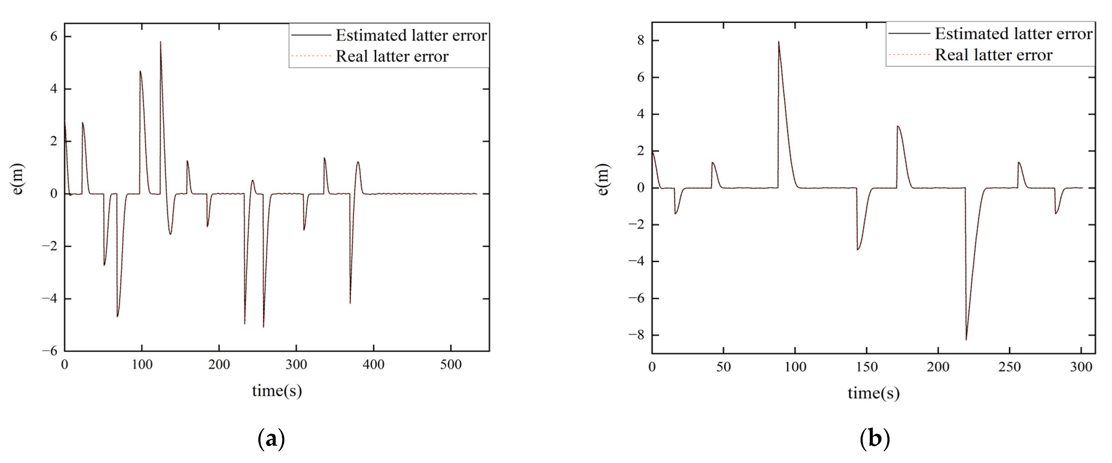
By comparing the estimated and actual values in Figure 8, it can be seen that the LESO designed in this paper was more effective and could estimate the lateral error in real time in the presence of interference, which also shows the rationality of the proposed control scheme.

To illustrate the advantage of the adopted ALOS algorithm with respect to the traditional LOS algorithm, the sum of absolute value of the lateral error of the whole process was used as a criterion to measure the ALOS algorithm $e_{sta}={\displaystyle \sum \left|e\right|}$, where $\Delta$ of LOS is a constant set as ${\Delta }_{\max }$. Calculated using path 1 as an example, the sum of the lateral error of ALOS was 430.8935 $\mathrm{m}$, while the sum of the lateral error of LOS was 432.0391 $\mathrm{m}$, which indicates that the adopted ALOS algorithm had higher accuracy and faster path-following speed. Since the difference between ALOS and LOS only appeared when the lateral error had a significant variation, the difference between the lateral error of the two was slight in this simulation experiment.

Figure 9 illustrates that the introduction of the ETM strategy reduced the computation of the control strategy to a certain extent, which could make up for the shortcomings of MPC’s extensive computation and improved the real-time performance to provide a way for practical application of the algorithm.

6. Conclusions

This paper focused on two hotly debated problems in USV control, i.e., path following and obstacle avoidance. The stability of the controller system designed in this paper was divided into three main components: ALOS stability, LESO stability, and MPC stability. Theoretically, the stability of the designed system was demonstrated in this paper. Several sets of comparative experiments were designed to illustrate the effectiveness and robustness of the proposed algorithm, mainly in four aspects. First, it was evident that the MPC controller had good control performance for actuator saturation and limiting compared with the PID controller. Therefore, using the MPC strategy reduced wear and tear. Second, LESO was designed to estimate the actual state quantities in order to resist the disturbance of external uncertainty and the effect of nonlinear model terms in the path-following process. The designed LESO was verified to have a good performance by simulation. Meanwhile, the designed LESO could ensure stability throughout the process during simulation experiments. Third, the ETM strategy was added to reduce the computational effort and improve the performance of practical applications. It is worth noting that the ETM strategy took effect when the desired path was not followed or the state error exceeded a set threshold, which also showed that the ETM strategy did not affect the system’s stability. On the contrary, it could also improve the system’s performance. The results show that the proposed algorithm could reduce the unnecessary computation of MPC while ensuring stability. Fourth, the proposed algorithm represents a geometric approach to solving the obstacle avoidance problem. Compared to Yao et al.’s work, for the known obstacles, the proposed algorithm avoided sensor accuracy and noise interference handling and further improved navigation safety. The effectiveness and robustness of the proposed algorithm were demonstrated through analyses of the following path and obstacle location.

In actual USV navigation, there may be a curved path to follow, which will be the focus of research in the future. At the same time, real ship experiments are expected to verify the application of the proposed algorithm in practical engineering. To better accomplish the obstacle avoidance task, the potential field’s theory can be added to the path replanning problem in future research. The previously established algorithms used in this paper, such as LESO and ETM strategies, can be further innovated in the future to better control the performance. Moreover, to design systems with better robustness, LESO can be used to design control rules that vary with disturbances.