Nonlinear Innovation-Based Maneuverability Prediction for Marine Vehicles Using an Improved Forgetting Mechanism

Abstract

This paper carries out marine vehicle maneuverability prediction based on nonlinear innovation. An improved Extended Kalman Filter (EKF) algorithm combined with a forgetting factor is developed by virtue of nonlinear innovation for ship maneuverability using full-scale data. Compared with existing algorithms, the proposed algorithm has high prediction consistency, a good prediction effect, and takes a shorter time to reach the agreement. Furthermore, the real-time prediction data are more than 95% consistent with the actual ship navigation. The forgetting factor is introduced to reduce the cumulative impact of historical interference data. Then, the tangent function is used to process errors; this can solve the problem of inaccurate maneuvering prediction of traditional identification algorithms, making up for the limitations of existing methods. The real-time prediction results are compared with the full-scale data, showing that the proposed ship prediction model has significant prediction accuracy and that the algorithm is reliable. This parameter identification method can be used to establish ship maneuvering prediction models.

1. Introduction

The EU Maritime Safety Agency has published an “Annual Overview of Maritime Casualties and Incidents 2020”, including an analysis of marine casualties and incidents reported by the EU in the European Maritime Accident Information Platform (EMCIP) as of 31 December 2020. In 2020, 2837 accidents were reported; the number of accidents in the previous six years was stable (an average of 3282 casualties from 2014 to 2019). In 2020, the total number of accidents stored in the EMCIP database exceeded 2250 [1].

In order to ensure the safety of navigation and to reduce ship collisions, ship motion pattern identification has become a popular research topic [2]. Maneuverability is an important identification object. As one of the ship’s hydrodynamic performance parameters, it is related to the safety and reliability of ship navigation. However, considering long-term ship operation, the performance of steering gear and hull resistance are time-varying, resulting in changes in ship maneuverability. Additionally, changes in the wave flow and ship draft will influence the ship’s maneuverability in real time [3]. This has a certain impact on accurate ship motion control using automatic rudders and advanced motion controllers (sliding mode control, model predictive control, etc.) that rely on ship maneuvering models. Therefore, it is necessary to realize the online identification of ship maneuvering model parameters and prediction [4,5,6]. Ship nonlinear motion model prediction is an important part of ship engineering research. Ship motion attitude prediction in waves usually refers to shortest-time prediction or real-time prediction; it predicts the ship’s motion attitude in a relatively short period of time in the future (3 to 10 s). Shortest-time prediction of ship motion has great military and civil value [7]; it plays an important role in ship safety and operation [8]. The mathematical model of ship motion is the basis and key to parameter identification and prediction. Establishing an accurate mathematical model of ship motion is essential for studying the ship’s motion characteristics [9].

In the three research fields of modern control systems (state estimation, identification, and control), system identification can effectively model the control process of uncertain or time-varying systems. The most commonly used identification methods are the least squares method [10], least squares recursive method [11,12], least squares support vector machine [13,14], random gradient algorithm [15], and neural networks based on identification algorithms [16]. Zhang, Zou [17], and Xu [18] used LSSVM and ε-LSSVM to research the modeling and prediction of ship maneuvering black boxes; Luo Weilin [19] used LSSVM to identify ship maneuverability parameters. The former research performed a regression analysis on the response relationship of ship motion characteristics from the perspective of black box modeling, and the latter gave a clear method for the determination of ship model parameters based on parameter identification.

The innovation identification theory uses certain-length information for recursive identification; by reusing the state information and measurement information, slow convergence speeds and low parameter identification accuracy can be improved to a certain extent [20]. Bai [21] identified this by locally weighted multi-innovation gradient iterative learning. Perez [22] studied model identification considering the actual measurement conditions of ship engineering. A two-step identification algorithm based on sensitivity weighting factors and the unscented Kalman filter has been proposed. Roth [23] used three common ship maneuverability prediction methods (automatic ship modeling tests, system prediction based on the computational fluid dynamics theory, and system simulations based on constrained ship modeling tests), combined with system identification technology to study the estimation of hydrodynamic derivatives in the ship design process.

The Kalman filtering algorithm is a recursive process. The current state of motion can be easily obtained by previous estimations of the motion state and the fixed prediction function [24]. Ship autonomous navigation control needs to establish an accurate model of ship maneuvering motion, and the identification of model parameters is an effective modeling method for control theory. As a filtering method that can predict and estimate the noise and state simultaneously, the Kalman filter (KF) has been applied to the parameter identification of ship motion models for a long time [25].

In 1992, Krstic used a direct MARC program and the inverse calculation of adjusting function to identify ship parameters [26]. Salid [27] proposed a 4-DOF model to avoid over-identification. In reference [28], the multi-innovation Kalman filter algorithm was used to track the target in video images, and the convergence of the proposed algorithm was proven by the approximation theory. The effectiveness of the multi-innovation Kalman Filter algorithm in tracking and prediction has been proven by simulation research. Nowadays, scholars mainly focus on the application of the improved Kalman filter in ship nonlinear models. Some have improved identification accuracy using Kalman smoothing filters on the identification data source [29], and some have changed the operation efficiency of the Kalman filtering algorithm itself [30]. However, the identification accuracy of EKF is sensitive to the initial estimation of process errors and measurement errors [31], and the algorithm is unstable and easy to diverge for the identification of strong nonlinear systems [32]. Many scholars have improved this, either by filtering the data source to improve the accuracy of EKF identification [33], or by parallel processing EKF to achieve efficient identification [34]. However, these algorithms do not pay attention to the real-time performance while improving the identification effect, which must be considered during actual navigation. The authors found that the existing prediction methods have a lot of room for improvement.

However, most identification results are based on non-interference motion model simulation data. In sensor measurements, the actual ship test data is not accurate enough. In order to improve the performance of covariance tracking, and to provide accurate parameter identification and the real-time prediction of ship models in ship autonomous navigation control, this paper proposes a real-time prediction method of nonlinear innovation ship maneuvering through full-scale test data based on a forgetting factor and Extended Kalman Filter.

Based on the above analysis, there are four main problems for identification method research: At present, research on ship motion identification modeling is mainly based on model simulation tests and scaled ship model tests—the scale effect is difficult to avoid. The effectiveness of the identification algorithm and the results’ accuracy need to be further improved.

Covariance matrices have the advantages of fusing multidimensional features to obtain a global optimal solution. However, traditional covariance matching is difficult to use for tracking severely occluded targets, and global searches are vulnerable to similar background interference.

Identification and prediction take a certain recursive time and need to converge and stabilize before a certain fitting degree is achieved. However, the convergence speed is too slow, and the fitting accuracy need to be improved.

In theory, there is a cumulative interference of old data for parameter estimation in the process of identification, and the data is not distinguished according to the degree of old and new—which is not conducive to the improvement of the convergence speed of identification, so as to reduce the prediction accuracy.

The main contributions of this paper are summarized as follows:

(1)

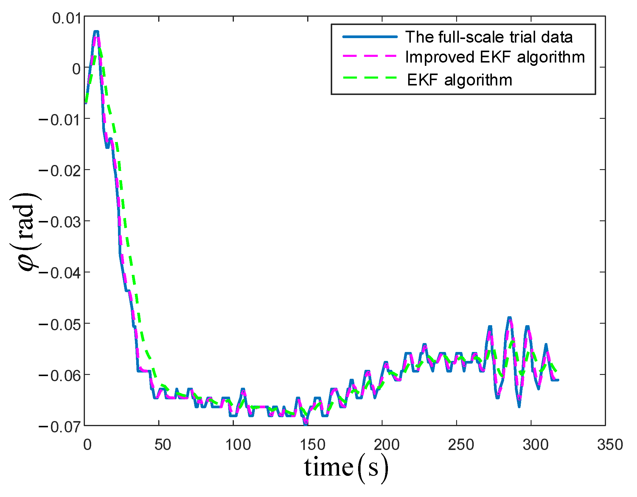
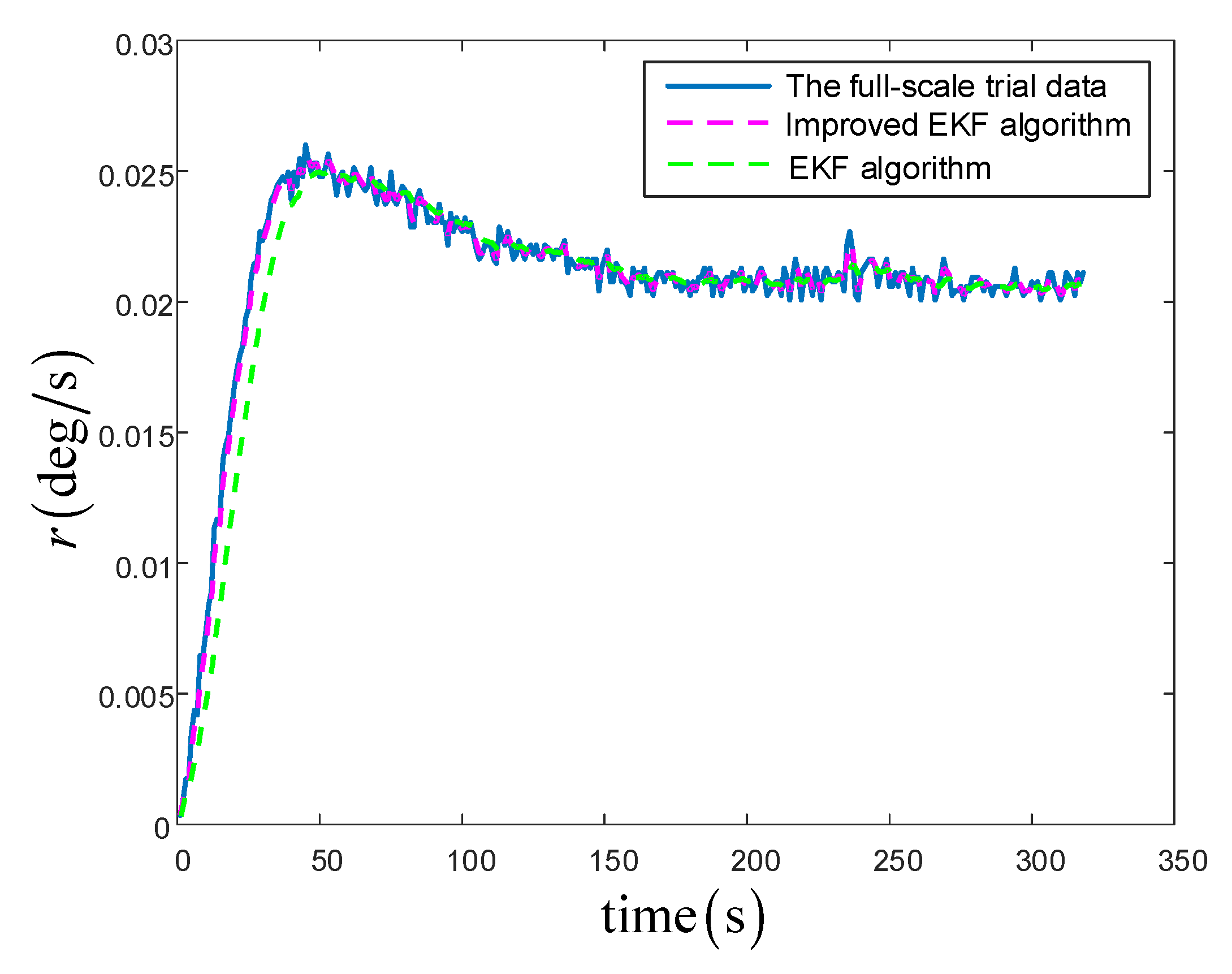
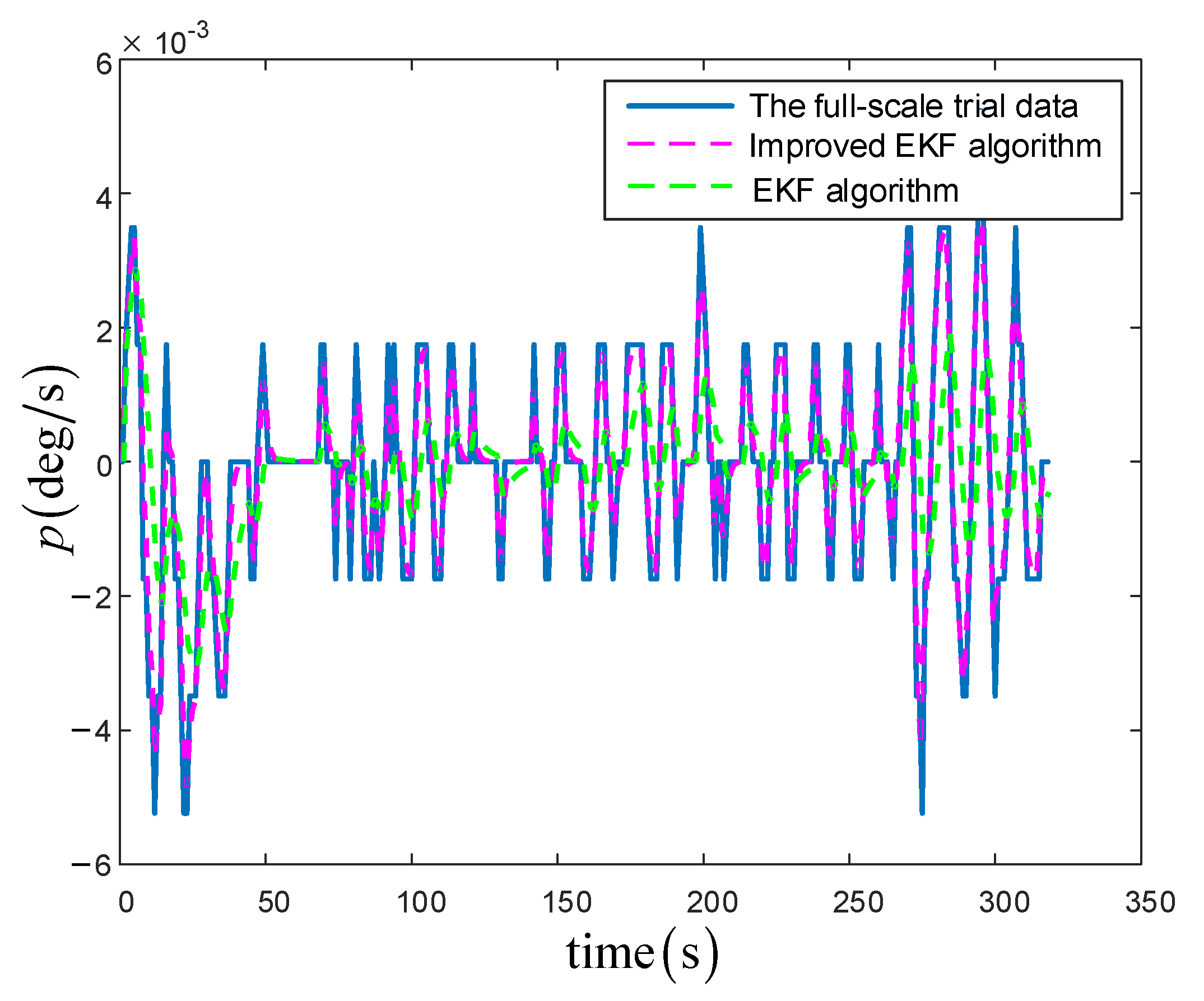
In this paper, an improved EFK algorithm was developed by virtue of nonlinear innovation. This solved the problem of limited innovation length for full-scale trail data and improved the online prediction convergence speed in engineering practice. Then, the tangent function was used to process errors. The forgetting factor was introduced to reduce the cumulative impact of historical interference data. The convergence of the improved algorithm identification and the consistency between the real-time prediction of ship maneuvering and the actual navigation were analyzed theoretically. In order to verify the effectiveness of the proposed method, this paper used real ship experimental data for turning tests. On this basis, the improved algorithm was compared with full-scale test data. The results showed that the proposed algorithm is effective, and that the real-time prediction data were more than 95% consistent with the ship’s actual navigation. This is more suitable for ship model parameter identification and maneuverability prediction. This has leading significance for practical engineering applications.

(2)

In this paper, a maneuvering prediction method was proposed for 4-DOF attitude prediction, using the corresponding nonlinear innovation algorithm. The parameters in the motion model were optimized to reduce the estimation error of the minimum variance, greatly improving the identification accuracy and efficiency. The most important purpose of this was to reduce the fitting time and improve the fitting degree. The effectiveness of this method for the real-time identification of ship motion mathematical model parameters was proven, and the feasibility of the ship motion prediction was verified. This method provides a theoretical reference for the real-time identification of actual ship motion.

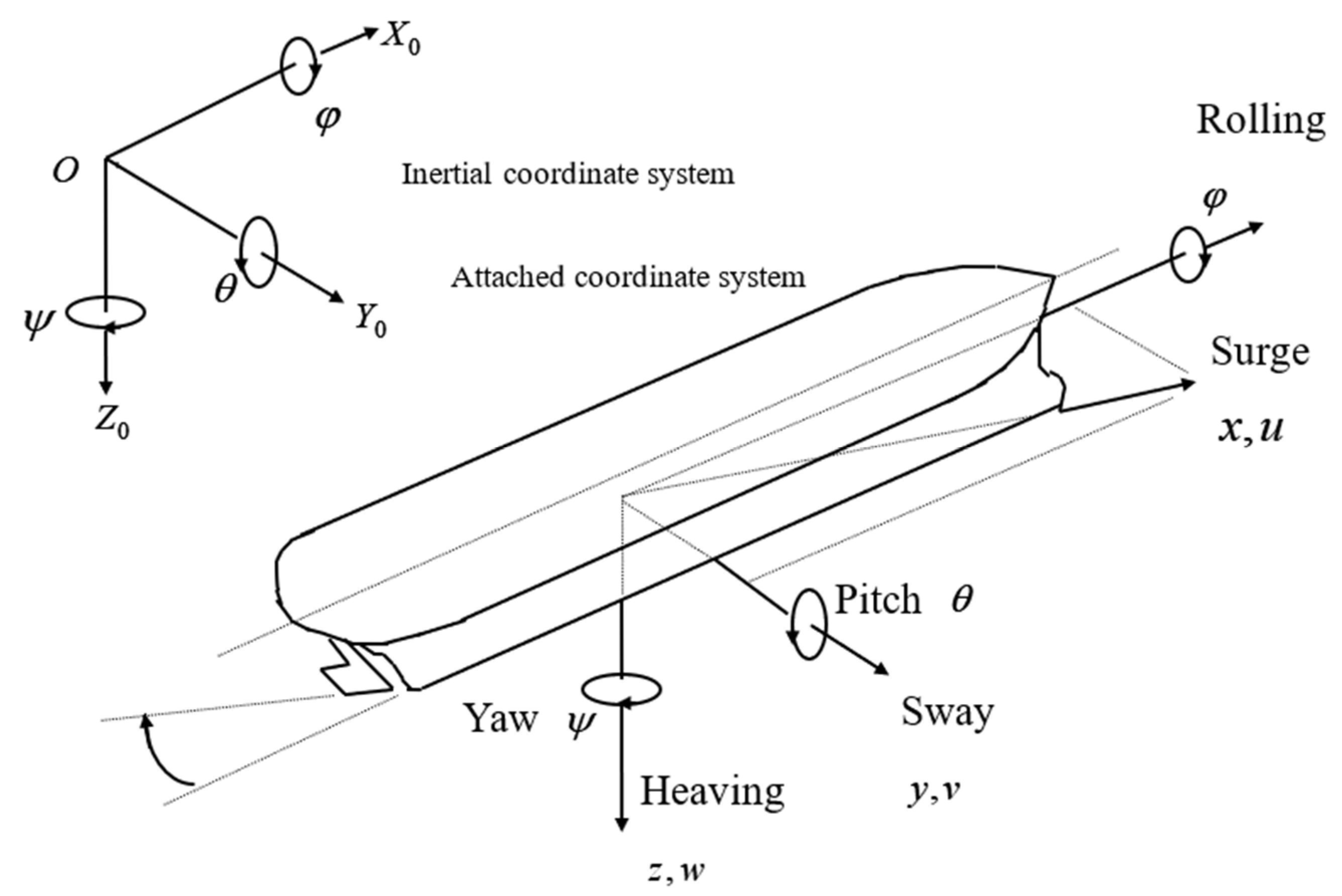
2. Description of the Mathematical Model

The Ship Maneuvering Mathematical Model Group (MMG) proposed a separate ship motion mathematical model. This model was designed to study the mutual interference between various parts in a propulsion and control system, based on the hydrodynamic characteristics of the hull, propeller, and rudder. Based on the MMG model and Newton’s rigid body mechanics, this paper established a mathematical model of ship motion with 4-DOF. The ship coordinate system is shown in Figure 1.

Where $u,v,r,p,\varphi$ denote the linear and angular velocities and roll angle, respectively; $m,I_x,I_z,m_x,m_y,J_x,J_z$ are the ship mass, the moments of inertia with respect to the x-axis and z-axis, and the corresponding added mass and added moment of inertia. GZ denotes the metacentric arm with respect to the x-axis. $g=9.8 \mathrm{N}/\mathrm{k}\mathrm{g}$ is the Newtonian universal of gravity. In addition, all of the above can be estimated with sufficient accuracy. In here, the damping force expression is used to describe the force or torque of the hull. These coefficients $X_H,Y_H,K_H,N_H$ are the hydrodynamic derivatives that will be estimated by the proposed identification scheme:

$$\begin{array}{l}\left(m+m_x\right)\dot{u}-\left(m+m_y\right)vr=X_H+X_P+X_R\\ \left(m+m_y\right)\dot{v}+\left(m+m_x\right)ur=Y_H+Y_P+Y_R\\ \left(I_x+J_x\right)\dot{p}-m_x{l}_{x}ur+mgGZ\left(\varphi \right)=K_H+K_P+K_R\\ \left(I_Z+J_Z\right)\dot{r}=N_H+N_P+N_R\end{array}$$

(1)

$$\begin{array}{l}{X}_H:u^2,u^3,v^2,r^2,vr,u{v}^2,uv{\varphi }^2,T\left(J_P\right),-F_N\sin \delta \\ Y_H:uv,up,u^{2}v,r^3,v{r}^2,uv{p}^2,ur{p}^2,\left|v\right|v,\left|r\right|v,\left|v\right|r,\left|r\right|r,-F_N\cos \delta \\ K_H:p,uv,ur,u^{2}v,v^3,v^{2}r,v{r}^2,uv{\varphi }^2,ur{\varphi }^2,\left|v\right|v,-F_N\cos \delta \\ N_H:uv,up,u\varphi ,u^{2}r,u^{2}v,v^3,r^3,v{r}^2,v^{2}r,ur{p}^2,\left|r\right|v,\left|v\right|v,-F_N\cos \delta \end{array}$$

(2)

The forces and moments of the propeller $X_P,Y_P,K_P,N_P$ and the rudder $X_R,Y_R,K_R,N_R$ are expressed as:

$$\begin{array}{l}{X}_P=\left(1-t_P\right)T\left(J_P\right),\\ Y_P=K_P=N_P=0,\\ X_R=-\left(1-t_R\right)F_N\sin \delta ,\\ Y_R=-\left(1+a_H\right)F_N\cos \delta ,\\ K_R=\left(1+a_H\right)Z_{HR}{F}_N\cos \delta ,\\ N_R=-\left(X_R+a_H{x}_H\right)F_N\cos \delta ,\\ T\left(J_P\right)=\rho \left|n\right|n{D}_P^4{K}_T\left(J_P\right),\\ K_T\left(J_P\right)=J_0+J_1{J}_P+J_2{J}_P^2\end{array}$$

(3)

$$\begin{array}{l}T\left(J_p\right)=\rho \left|n\right|n{D}_P^4{K}_T\left(J_p\right)\\ K_T\left(J_p\right)=J_0+J_1{J}_p+J_2{J}_p^2\end{array}$$

(4)

where $t_P,n,D_P,K_T,J_P$ are the thrust deduction fractions, propeller revolutions per second, propeller diameter, the thrust coefficient, and the advance ratio of propeller, respectively; $J_0,J_1,J_2$ are the hydrodynamic coefficients for the open water propeller characteristics. For the rudder force/moment, $\delta ,x_R,z_{HR}$ denote the rudder angle, the $x$ and $z$ directional center of the normal force acting on the rudder. Additionally, $t_R,a_H,x_H$ are used to describe the interaction of the hull and rudder. In the identification scheme, the parameters in the equation $\left(1-t_R\right),\left(1+a_H\right),\left(1+a_H\right)z_{HR},\left(x_R+a_H{x}_H\right)$ are considered as coefficients to be estimated.

The mathematical model Equations (1)–(4) provide a generalized family model that can describe nonlinear dynamics of different ships.

3. Design of the Nonlinear Innovation Based on the Identification Algorithm

In order to identify the ship motion model of the state space type, six categories of data are needed. The speed $u$, the sway velocity $v$, the rolling rate $p$, the yaw rate $r$, the propeller velocity $n$, and the rudder angle $\delta$. These time series are the measured data from the ship’s actual navigation. The model parameters that need to be identified in Equation (5) are $a_i\left(i=1~9\right),b_i\left(i=1~12\right),c_i\left(i=1~11\right),d_i\left(i=1~13\right)$—45 parameters in total.

$$\begin{array}{l}\dot{u}=a_1{u}^2+a_2{u}^3+a_3{v}^2+a_4{r}^2+a_{5}vr+a_{6}u{v}^2+a_{7}uv{\varphi }^2+a_{8}T\left(J_p\right)+a_9{F}_N\sin \delta \\ \dot{v}=b_{1}uv+b_{2}up+b_3{u}^{2}v+b_4{r}^3+b_{5}v{r}^2+b_{6}uv{p}^2+b_{7}ur{p}^2+b_8\left|v\right|v+b_9\left|r\right|v+\\ b_{10}\left|v\right|r+b_{11}\left|r\right|r-b_{12}{F}_N\cos \delta \\ \dot{p}=c_{1}p+c_{2}uv+c_{3}ur+c_4{u}^{2}v+c_5{v}^3+c_6{v}^{2}r+c_{7}v{r}^2+c_{8}uv{\varphi }^2+c_{9}ur{\varphi }^2+\\ c_{10}\left|v\right|v-c_{11}{F}_N\cos \delta \\ \dot{r}=d_{1}uv+d_{2}up+d_{3}u\varphi +d_4{u}^{2}r+d_5{u}^{2}v+d_6{v}^3+d_7{r}^3+d_{8}v{r}^2+d_9{v}^{2}r+\\ d_{10}ur{p}^2+d_{11}\left|r\right|v+d_{12}\left|v\right|v-d_{13}{F}_N\cos \delta \end{array}$$

(5)

Reducing Equation (5) to a general system equation:

$$\begin{array}{l}\dot{x}(t)=\left[f\left(x\left(t\right),s\left(t\right),t\right)+\omega \left(t\right)\tan \left(\omega e\right)\right]{\mathbf{\alpha }}^{*}\\ y\left(t\right)=\left[Hx\left(t\right)+e\left(t\right)\tan \left(\omega e\right)\right]{\mathbf{\alpha }}^{*}\end{array}$$

(6)

In Equation (6), $x\left(t\right)={\left[\begin{array}{cccc}u\left(t\right)& v\left(t\right)& p\left(t\right)& r\left(t\right)\end{array}\right]}^{\mathrm{T}},s\left(t\right)={\left[\begin{array}{cc}\delta \left(t\right)& n\left(t\right)\end{array}\right]}^{\mathrm{T}},$ $f={\left[\begin{array}{cccc}{f}_1& f_2& f_3& f_4\end{array}\right]}^{\mathrm{T}},$$H=I_{4\times 4}$.

When the number of innovations continues to increase, the cumulative interference of old information rises, and the estimation error of the algorithm begins to increase.

The forgetting factor is introduced to identify and improve the algorithm. By weakening the historical old data, the correction effect is enhanced, and the cumulative interference is reduced. The algorithm reacts quickly to changes in new measurement inputs.

The forgetting factor matrix $\mathbf{\alpha }$ is added to the matrix in Equation (6) to reduce the weight of the information and to increase the weight of new measurement information, so as to improve the algorithm and define the matrix. In order to maximize the gain weight of information, it can be described as in Equation (7):

$${\mathit{\lambda }}_1\ge \left({\mathit{\lambda }}_2+{\mathit{\lambda }}_3+\cdot \cdot \cdot +{\mathit{\lambda }}_p\right)$$

(7)

After weighting and processing the old information gain, the algorithm achieves a relative balance between effective correction and inhibition of cumulative interference. In order to further improve the method, Equation (8) can be written as:

$$\{\begin{array}{c}{\mathit{\lambda }}_1=1\\ {\mathit{\lambda }}_2={\mathit{\lambda }}_3=\cdot \cdot \cdot ={\mathit{\lambda }}_p=\frac{\alpha }{p-1},0<\alpha <1\end{array}$$

(8)

In Equation (8): $\alpha$ is the design parameter of the forgetting factor matrix. When the parameter is $0<\alpha <1$, the equation holds. $\alpha =0$ is meaningless and $\alpha =1$ means no forgetting. The smaller the parameter, the more information is forgotten.

The model parameters $a_i,b_i,c_i,d_i$ are introduced into the Extended Kalman Filtering algorithm as an unknown quantity. These are state variables of the Extended Kalman Filter algorithm that identify the model parameters of the separated ship motion model. The state equation and observation equation of the extended system are discretized as follows (9):

Based on the EKF algorithm and forgetting factor, combined with the nonlinear innovation algorithm, an improved algorithm is formed:

$$\begin{array}{l}{\dot{x}}^a(t+1)=\left[f^a\left(x^a\left(t\right),s\left(t\right),t\right)+\omega \left(t\right)\tan \left(\omega e\right)\right]{\mathbf{\alpha }}^{*}\\ y\left(t\right)=\left[H{x}^a\left(t\right)+e\left(t\right)\tan \left(\omega e\right)\right]{\mathbf{\alpha }}^{*}\end{array}$$

(9)

In Equation (9), $s\left(t\right)$ represents the sampling mean of the input at $T\left(t\right)$ and $T\left(t+1\right)$, $T$ is the sampling interval, $w\left(t\right)$ is the zero-mean white noise sequence, $e\left(t\right)$ is the error (innovation), and the variances are $Q$ and $R$, respectively; $f^a={\left[f_1^a{f}_2^a...f_{45}^a\right]}^{\mathrm{T}}$. According to Equations (5) and (9), the following expression is obtained:

$$\begin{array}{l}{f}_1^a=T\left(\begin{array}{l}{a}_1\left(t\right)u{\left(t\right)}^2+a_2\left(t\right)u{\left(t\right)}^3+a_3\left(t\right)v{\left(t\right)}^2+a_4\left(t\right)r{\left(t\right)}^2+a_5\left(t\right)v\left(t\right)r\left(t\right)+\\ a_{6}u\left(t\right)v{\left(t\right)}^2+a_7\left(t\right)u\left(t\right)v\left(t\right)\varphi {\left(t\right)}^2+a_8\left(t\right)T\left(J_p\right)\left(t\right)+a_9\left(t\right)F_N\sin \delta \left(t\right)\end{array}\right)\\ f_2^a=T\left(\begin{array}{l}{b}_1\left(t\right)u\left(t\right)v\left(t\right)+b_2\left(t\right)u\left(t\right)p\left(t\right)+b_3\left(t\right)u{\left(t\right)}^{2}v\left(t\right)+b_4\left(t\right)r{\left(t\right)}^3+\\ b_5\left(t\right)v\left(t\right)r{\left(t\right)}^2+b_6\left(t\right)u\left(t\right)v\left(t\right)p{\left(t\right)}^2+b_7\left(t\right)u\left(t\right)r\left(t\right)p{\left(t\right)}^2+\\ b_8\left(t\right)\left|v\right|\left(t\right)v\left(t\right)+b_9\left(t\right)\left|r\right|\left(t\right)v\left(t\right)+b_{10}\left(t\right)\left|v\right|\left(t\right)r\left(t\right)+b_{11}\left(t\right)\left|r\right|\left(t\right)r\left(t\right)-\\ b_{12}\left(t\right)F_N\cos \delta \left(t\right)\end{array}\right)\\ f_3^a=T\left(\begin{array}{l}{c}_1\left(t\right)p\left(t\right)+c_2\left(t\right)u\left(t\right)v\left(t\right)+c_3\left(t\right)u\left(t\right)r\left(t\right)+c_4\left(t\right)u{\left(t\right)}^{2}v\left(t\right)+\\ c_5\left(t\right)v{\left(t\right)}^3+c_6\left(t\right)v{\left(t\right)}^{2}r\left(t\right)+c_7\left(t\right)v\left(t\right)r{\left(t\right)}^2+c_8\left(t\right)u\left(t\right)v\left(t\right)\varphi {\left(t\right)}^2+\\ c_9\left(t\right)u\left(t\right)r\left(t\right)\varphi {\left(t\right)}^2+c_{10}\left(t\right)\left|v\right|\left(t\right)v\left(t\right)-c_{11}\left(t\right)F_N\cos \delta \left(t\right)\end{array}\right)\\ f_4^a=T\left(\begin{array}{l}{d}_1\left(t\right)u\left(t\right)v\left(t\right)+d_2\left(t\right)u\left(t\right)p\left(t\right)+d_3\left(t\right)u\left(t\right)\varphi \left(t\right)+d_4\left(t\right)u{\left(t\right)}^{2}r\left(t\right)+\\ d_5\left(t\right)u{\left(t\right)}^{2}v\left(t\right)+d_6\left(t\right)v{\left(t\right)}^3+d_7\left(t\right)r{\left(t\right)}^3+d_8\left(t\right)v\left(t\right)r{\left(t\right)}^2+\\ d_9\left(t\right)v{\left(t\right)}^{2}r\left(t\right)+d_{10}\left(t\right)u\left(t\right)r\left(t\right)p{\left(t\right)}^2+d_{11}\left(t\right)\left|r\right|\left(t\right)v\left(t\right)+\\ d_{12}\left(t\right)\left|v\right|\left(t\right)v\left(t\right)-d_{13}\left(t\right)F_N\cos \delta \left(t\right)\end{array}\right)\\ f_5^a=a_1\left(t\right),f_6^a=a_2\left(t\right),...,f_{49}^a=d_{13}\left(t\right)\end{array}$$

(10)

The improved recursive equation can be expressed as:

$$\begin{array}{l}{\widehat{X}}^a\left(t+1|t\right)=f^a\left(x^a\left(t\right),s\left(t\right),t\right)\tan \left(\omega e\right){\mathbf{\alpha }}^{*}\\ P\left(t+1|t\right)=\left(\mathbf{\Phi }P\left(t\right){\mathbf{\Phi }}^{\mathrm{T}}+Q\right){\mathbf{\alpha }}^{*}\\ K\left(t+1\right)=P\left(t+1|t\right)H^{\mathrm{T}}{\left[HP\left(t+1|t\right)H^{\mathrm{T}}+R\right]}^{-1}\\ P\left(t+1\right)=\left[I-K\left(t+1\right)H\right]P\left(t+1|t\right)\\ \widehat{X}\left(t+1\right)=\widehat{X}\left(t+1|t\right)+K\left(t+1\right)\cdot \left[y\left(t+1\right)-H\widehat{X}\left(t+1|t\right)\right]\tan \left(\omega e\right){\mathbf{\alpha }}^{*}\end{array}$$

(11)

Remark 1.

The forgetting factor is introduced to reduce the cumulative impact of historical interference data.

Remark 2.

The improved Extended Kalman filter is introduced to optimize the parameters in the motion model, which reduces the estimation error of the minimum variance, shortens the fitting time, and improves the fitting degree.

In Equation (11), ${\mathbf{\Phi }}_{45\times 45}=\frac{\partial f^a}{\partial x^a}{|}_{x^a=x^a\left(k\right)}$. After repeated recursion, the system will reach a convergence state; then, the state value $x^a\left(t\right)$ of Equation (9) can be obtained, so as to obtain the estimated value of the model parameter $a_i,b_i,c_i,d_i$.

In order to better illustrate that the motion model established by identifying model parameters can more accurately reflect the motion time data sequence, the fitted motion model is established with the identified data of each step. In the test, the prior identification data are used in the previous step, and the identified parameters are used for estimation in the next step. Firstly, the nonlinear ship motion parameter identification model is established:

$$\begin{array}{l}\dot{u}=a_1\left(t\right)u^2+a_2\left(t\right)u^3+a_3\left(t\right)v^2+a_4\left(t\right)r^2+a_5\left(t\right)vr+a_{6}u{v}^2+a_7\left(t\right)uv{\varphi }^2+\\ a_8\left(t\right)T\left(J_p\right)+a_9\left(t\right)F_N\sin \delta \\ \dot{v}=b_1\left(t\right)uv+b_2\left(t\right)up+b_3\left(t\right)u^{2}v+b_4\left(t\right)r^3+b_5\left(t\right)v{r}^2+b_6\left(t\right)uv{p}^2+\\ b_7\left(t\right)ur{p}^2+b_8\left(t\right)\left|v\right|v+b_9\left(t\right)\left|r\right|v+b_{10}\left(t\right)\left|v\right|r+b_{11}\left(t\right)\left|r\right|r-b_{12}\left(t\right)F_N\cos \delta \\ \dot{p}=c_1\left(t\right)p+c_2\left(t\right)uv+c_3\left(t\right)ur+c_4\left(t\right)u^{2}v+c_5\left(t\right)v^3+c_6\left(t\right)v^{2}r+c_7\left(t\right)v{r}^2+\\ c_8\left(t\right)uv{\varphi }^2+c_9\left(t\right)ur{\varphi }^2+c_{10}\left(t\right)\left|v\right|v-c_{11}\left(t\right)F_N\cos \delta \\ \dot{r}=d_1\left(t\right)uv+d_2\left(t\right)up+d_3\left(t\right)u\varphi +d_4\left(t\right)u^{2}r+d_5\left(t\right)u^{2}v+d_6\left(t\right)v^3+\\ d_7\left(t\right)r^3+d_8\left(t\right)v{r}^2+d_9\left(t\right)v^{2}r+d_{10}\left(t\right)ur{p}^2+d_{11}\left(t\right)\left|r\right|v+d_{12}\left(t\right)\left|v\right|v-d_{13}\left(t\right)F_N\cos \delta \end{array}$$

(12)

This is a nonlinear time-varying model and the model parameters change over time. According to the step length of the identification data $h=1 \mathrm{s}$, Equation (13) is discretized to obtain:

$$\begin{array}{l}u\left(t+1\right)=u\left(t\right)+h\times \left(\begin{array}{l}{a}_1\left(t\right)u^2\left(t\right)+a_2\left(t\right)u^3\left(t\right)+a_3\left(t\right)v^2\left(t\right)+a_4\left(t\right)r^2\left(t\right)+\\ a_5\left(t\right)v\left(t\right)r\left(t\right)+a_{6}u\left(t\right)v^2\left(t\right)+a_7\left(t\right)u\left(t\right)v\left(t\right){\varphi }^2\left(t\right)+\\ a_8\left(t\right)T\left(J_p\right)\left(t\right)+a_9\left(t\right)F_N\sin \delta \left(t\right)\end{array}\right)\\ v\left(t+1\right)=v\left(t\right)+h\times \left(\begin{array}{l}{b}_1\left(t\right)u\left(t\right)v\left(t\right)+b_2\left(t\right)u\left(t\right)p\left(t\right)+b_3\left(t\right)u^2\left(t\right)v\left(t\right)+\\ b_4\left(t\right)r^3\left(t\right)+b_5\left(t\right)v\left(t\right)r^2\left(t\right)+b_6\left(t\right)u\left(t\right)v\left(t\right)p^2\left(t\right)+\\ b_7\left(t\right)u\left(t\right)r\left(t\right)p^2\left(t\right)+b_8\left(t\right)\left|v\right|\left(t\right)v\left(t\right)+b_9\left(t\right)\left|r\right|\left(t\right)v\left(t\right)+\\ b_{10}\left(t\right)\left|v\right|\left(t\right)r\left(t\right)+b_{11}\left(t\right)\left|r\right|\left(t\right)r\left(t\right)-b_{12}\left(t\right)F_N\cos \delta \left(t\right)\end{array}\right)\\ p\left(t+1\right)=p\left(t\right)+h\times \left(\begin{array}{l}{c}_1\left(t\right)p\left(t\right)+c_2\left(t\right)u\left(t\right)v\left(t\right)+c_3\left(t\right)u\left(t\right)r\left(t\right)+\\ c_4\left(t\right)u^2\left(t\right)v\left(t\right)+c_5\left(t\right)v^3\left(t\right)+c_6\left(t\right)v^2\left(t\right)r\left(t\right)+\\ c_7\left(t\right)v\left(t\right)r^2\left(t\right)+c_8\left(t\right)u\left(t\right)v\left(t\right){\varphi }^2\left(t\right)+\\ c_9\left(t\right)u\left(t\right)r\left(t\right){\varphi }^2\left(t\right)+c_{10}\left(t\right)\left|v\right|\left(t\right)v\left(t\right)-\\ c_{11}\left(t\right)F_N\cos \delta \left(t\right)\end{array}\right)\\ r\left(t+1\right)=r\left(t\right)+h\times \left(\begin{array}{l}{d}_1\left(t\right)u\left(t\right)v\left(t\right)+d_2\left(t\right)u\left(t\right)p\left(t\right)+d_3\left(t\right)u\left(t\right)\varphi \left(t\right)+\\ d_4\left(t\right)u^2\left(t\right)r\left(t\right)+d_5\left(t\right)u^2\left(t\right)v\left(t\right)+d_6\left(t\right)v^3\left(t\right)+\\ d_7\left(t\right)r^3\left(t\right)+d_8\left(t\right)v\left(t\right)r^2\left(t\right)+d_9\left(t\right)v^2\left(t\right)r\left(t\right)+\\ d_{10}\left(t\right)u\left(t\right)r\left(t\right)p^2\left(t\right)+d_{11}\left(t\right)\left|r\right|\left(t\right)v\left(t\right)+d_{12}\left(t\right)\left|v\right|\left(t\right)v\left(t\right)-\\ d_{13}\left(t\right)F_N\cos \delta \left(t\right)\end{array}\right)\end{array}$$

(13)

The convergence of the filter state estimation directly affects the reliability of the filter identification. The basic measure to improve the filter convergence is to properly increase the weighting of the innovation $e\left(t\right)=y\left(t\right)-C\widehat{x}\left(t|t-1\right)$ to ensure that the gain matrix $T\left(t+1\right)$ has sufficient strength, so that the forecast $\widehat{x}\left(t|t-1\right)$ can be corrected in time.

Among these,

State prediction:

$$\widehat{x}\left(t+1|t\right)=\left(\mathbf{\Phi }\widehat{x}\left(t\right)+GU\left(t\right)\right){\mathbf{\alpha }}^{*}$$

(14)

Innovation:

$$e\left(t+1\right)=y\left(t+1\right)-C\widehat{x}\left(t-1|t\right)$$

(15)

Prediction error covariance matrix:

$$P\left(t+1|t\right)=\left[M\left(t+1\right)\mathbf{\Phi }P\left(t\right){\mathbf{\Phi }}^{\mathrm{T}}+R_1\left(t\right)\right]{\mathbf{\alpha }}^{*}$$

(16)

Logical calculation according to guaranteed convergence measures $M\left(t+1\right)$.

Filter gain matrix:

$$K\left(t+1\right)=P\left(t+1|t\right)C^{\mathrm{T}}{\left[CP\left(t+1|t\right)C^{\mathrm{T}}+R_2\left(t\right)\right]}^{-1}$$

(17)

State estimation:

$$\widehat{x}\left(t+1\right)=\left[\widehat{x}\left(t+1|t\right)+K\left(t+1\right)e\left(t+1\right)\right]{\mathbf{\alpha }}^{*}$$

(18)

Estimated error covariance matrix:

$$P\left(t+1\right)=\left[I-K\left(t+1\right)C\right]P\left(t+1|t\right){\mathbf{\alpha }}^{*}$$

(19)

It can be seen that Equation (16) has only one more coefficient M(k + 1) that guarantees convergence other than the general Kalman filter equation. The value of M(k + 1) is calculated according to the Kalman filter convergence condition. Convergence condition 1 is:

$$e^{\mathrm{T}}\left(t\right)e\left(t\right)\le t_r\left[\mathrm{Var}\left[e\left(t\right)\right]\right]=t_r\left[CP\left(t|t-1\right)C^{\mathrm{T}}+R_1\left(t\right)\right]$$

(20)

If Equation (20) holds, then convergence, otherwise it diverges.

Convergence condition 2 is:

$$e^{\mathrm{T}}\left(t\right)e\left(t\right)<\mathrm{Var}\left[e\left(t\right)\right]=CP\left(t|t-1\right)C^{\mathrm{T}}+R_1\left(t\right)$$

(21)

If Equation (21) holds, then it converges, otherwise it diverges.

Using convergence condition 1 to judge whether the parameter identification of the improved algorithm converges, and using condition 2 to calculate $M\left(t+1\right)$,

$$e^{\mathrm{T}}\left(t\right)e\left(t\right)\le t_r\left\{C\left[\mathbf{\Phi }P\left(t\right){\mathbf{\Phi }}^{\mathrm{T}}+R_1\left(t\right)\right]C^{\mathrm{T}}+R_2\left(t\right)\right\}$$

(22)

If Equation (22) inequality holds, then it converges; then $M\left(t+1\right)=1$.

Otherwise it diverges, and then:

$$M\left(t+1\right)=\frac{1}{n}{t}_r\left\{\left[e^{\mathrm{T}}\left(t+1\right)e\left(t+1\right)-C{R}_1\left(t\right)C^{\mathrm{T}}-R_2\left(t\right)\right]{\left[C\mathbf{\Phi }P\left(t\right){\mathbf{\Phi }}^{\mathrm{T}}{C}^{\mathrm{T}}\right]}^{-1}\right\}$$

(23)

where $n$ is the filter dimension.

4. Experiment for the Maneuvering Prediction and Discussion

The identification modeling needs prior data as the identification data. The prior data can be the actual ship data or the simulation results. This paper is based on full-scale actual ship test data. Actual ship experimental data can better reflect the real situation of ship navigation and is more representative.

The data used in this paper are from the “Yukun” ship sea test. The “Yukun” ship is a scientific research and training ship of Dalian Maritime University. Its main parameters are shown in

Table 1. The Principal Particulars of the Vessel “Yukun”.

Quantity	Conversion from Gaussian and CGS EMU to SI
Length between perpendiculars	$105 \mathrm{m}$
Breadth	$18 \mathrm{m}$
Mean draft	$5.4 \mathrm{m}$
Displacement volume	$5710.2 {\mathrm{m}}^3$
Height of the initial stability	$1.3 \mathrm{m}$
Block coefficient	$0.5595$
Rudder area	$11.8 {\mathrm{m}}^2$
Aspect ratio	$1.9525$
Max. rudder angle	$30°$
Max. rudder rate	$2.8°/\mathrm{s}$
Propeller diameter	$3.8 \mathrm{m}$
Speed	$16.7 \mathrm{kn}$
Max. shaft velocity	$120 \mathrm{rpm}$

. Ship turning tests are used to evaluate ship maneuverability. Figure 2 shows the turning test of the “Yukun” ship in the Bohai Sea.

The operation speed of the “Yukun” ship is $16.7 \mathrm{kn}$, but in this test, in order to prove the accuracy of the real-time prediction to a greater extent, the speed was increased to $18.5 \mathrm{kn}$.

A comparison of the results from EKF algorithm and the improved algorithm is shown in Figure 3, Figure 4 and Figure 5; it can be seen that the traditional method (EKF algorithm) has low prediction accuracy, poor prediction coincidence, slow fitting speed, and a certain deviation from the real values.

The average error between the trail data and predicted data was 1.31% in the rolling angle, 0.4% in the yaw rate, and 9.65% in the rolling rate. It can be seen from the above that the proposed algorithm not only has high accuracy and better convergence, but most importantly, that the results were highly fitted to the true values. Furthermore, the convergence time was short and had better prediction results. These results are sufficient to prove that the algorithm is reliable in terms of parameter identification and prediction.

5. Conclusions

In this paper, a marine vehicle maneuverability prediction method based on nonlinear innovation was proposed. This was an improved Extended Kalman Filter (EKF) algorithm combined with a forgetting factor. Based on the existing EKF algorithm, a forgetting factor was introduced to reduce the cumulative impact of historical interference data. Then, the tangent function was used to process errors. The experimental results showed that the prediction consistency of the proposed algorithm was more than 95%. This algorithm greatly improved prediction speed and accuracy. This proves that the method can feasibly provide real-time prediction in actual ship navigation. With the development of large-scale and intelligent ships, ships in different navigation environments need real-time precise motion models of ships. The method proposed in this paper can provide a theoretical reference to improve the control level of ships.

Next, the authors will carry out more tests for unmanned ships, so that the ship decision system can be better applied in the direction of unmanned ships.

References

1. Duncombe, J.U. Infrared navigation—Part I: An assessment of feasibility. IEEE Trans. Electron Devices 1959, ED-11, 34–39. [Google Scholar] [CrossRef]
2. Guo, J.; Chiu, F.C.; Cheng, S.W.; Chen, H.W. Docking control for a biomimetic autonomous underwater vehicle using active vision. IFAC Proc. Vol. 2006, 3916, 335–347. [Google Scholar] [CrossRef]
3. Song, C.; Zhang, X.; Zhang, G. Nonlinear innovation identification of ship response model via the hyperbolic tangent function. Proc. Inst. Mech. Eng. Part I J. Syst. Control. Eng. 2021, 235, 977–983. [Google Scholar] [CrossRef]
4. Parczewski, K.; Wnk, H. The influence of vehicle body roll angle on the motion stability and maneuverability of the vehicle. Combust. Engines 2017, 56, 133–139. [Google Scholar] [CrossRef]
5. Hu, J.; Bu, R.; Yin, J.; Wang, Y. Adaptive control for ship steering based on clonal selection model identification. In Proceedings of the 2009 Chinese Control and Decision Conference, Guilin, China, 17–19 June 2009; pp. 2863–2868. [Google Scholar]
6. Sonnenburg, C.R.; Woolsey, C.A. Modeling, identification, and control of an unmanned surface vehicle. J. Field Robot. 2013, 30, 371–398. [Google Scholar] [CrossRef]
7. Van Gestel, T.; De Brabanter, J.; De Moor, B.; Vandewalle, J.; Suykens, J.A.K.; Van Gestel, T. Least Squares Support Vector Machines; World Scientific: Singapore, 2002. [Google Scholar]
8. Zhang, X.-K.; Zhang, G.-Q.; Ren, H.-X.; Yang, G.-P. Linear reduction of backstepping algorithm based on nonlinear decoration for ship course-keeping control system. Ocean. Eng. 2018, 147, 1–8. [Google Scholar] [CrossRef]
9. Qin, Y.; Ma, Y. Parametric Identification of ship’s Maneuvering Motion Based on Improved Least Square Method. In Proceedings of the 2014 International Conference on Mechatronics, Electronic, Industrial and Control Engineering (MEIC-14), Shenyang, China, 15–17 November 2014; Atlantis Press: Amsterdam, The Netherlands, 2014. [Google Scholar]
10. Hu, Y.; Xu, S. A direct generalized predictive controller for ship course keeping. In Proceedings of the 2007 Mediterranean Conference on Control & Automation, Athens, Greece, 27–29 June 2007; pp. 1–4. [Google Scholar]
11. Xie, S.; Chu, X.; Liu, C.; Wang, L.; Mao, W. Ship heading control based on backstepping and Least squares support vector machine. In Proceedings of the 2017 4th International Conference on Transportation Information and Safety (ICTIS), Banff, AB, Canada, 8–10 August 2017. [Google Scholar]
12. Chunyu, S.; Zhang, X.; Zhang, G. Nonliner Identification For 4 DOF Ship Maneuvering Modeling Via Full-Scale Trial Data. IEEE Trans. Ind. Electron. 2021, 69, 1829–1835. [Google Scholar]
13. Hess, D.; Faller, W. Simulation of ship maneuvering using recursive neural networks. In Proceedings of the 23rd Symposium on Naval Hydrodynamics, Val de Reuil, France, 17–22 September 2000. [Google Scholar]
14. Zhang, X.; Wang, X.; Meng, Y.; Yin, Y. Research progress and future development trend of ship motion modeling and simulation. J. Dalian Marit. Univ. 2021, 47, 1–8. [Google Scholar]
15. Zhang, G.Q.; Zhang, X.K.; Pang, H.S. Multi-innovation auto-constructed least squares identification for 4 DOF ship maneuvering modelling with full-scale trial data. Isa Trans. 2015, 58, 186–195. [Google Scholar] [CrossRef]
16. Xie, L.B.; Feng, D.; Wang, Y. Auxiliary model-based identification method for quantized control systems. Kongzhi Lilun Yu Yinyong/Control. Theory Appl. 2009, 26, 277–282. [Google Scholar]
17. Ruichek, Y. Multilevel- and neural-network-based stereo-matching method for real-time obstacle detection using linear cameras. IEEE Trans. Intell. Transp. Syst. 2005, 6, 54–62. [Google Scholar] [CrossRef]
18. Zhang, X.G.; Zou, Z.J. Black-box modeling of nonlinear hydrodynamic model for ship maneuvering based on support-vector-regression. In Proceedings of the International Conference on Marine Simulation and Ship Maneuverability 2012 (MARSIM 2012), Singapore, 23–27 April 2012. [Google Scholar]
19. Zhang, X.G.; Zou, Z.J. Black box modeling of ship maneuvering motion based on support vector machine. J. Beijing Univ. Aeronaut. Astronsutics 2013, 11, 025. [Google Scholar]
20. Xie, S.; Chen, D.; Chu, X.; Liu, C. Improved multi-innovation Kalman filter method to identify ship response model. J. Harbin Eng. Univ. 2018, 39, 8. [Google Scholar]
21. Bai, W.; Ren, J. Multi-Innovation Gradient Iterative Locally Weighted Learning Identification for A Nonlinear Ship Maneuvering System. China Ocean. Eng. 2018, 32, 288–300. [Google Scholar] [CrossRef]
22. Perez, T.; Fossen, T. Time-domain models of marine surface vessels based on seakeeping computations. In Proceedings of the 7th IFAC Conference on Maneuvering and Control of Marine Vessels MCMC, Lisbon, Portugal, 20–22 September 2006. [Google Scholar]
23. Ross, A. Nonlinear Maneuvering Models for Ships: A Lagrangian Approach. Ph.D. Thesis, Norwegian University of Science and Technology, Trondheim, Norway, 2008. [Google Scholar]
24. Randeni, P.S.; Forrest, A.L.; Cossu, R.; Leong, Z.Q.; Ranmuthugala, D.; Schmidt, V. Parameter identification of a nonlinear model: Replicating the motion response of an autonomous underwater vehicle for dynamic environments. Nonlinear Dyn. 2018, 91, 1229–1247. [Google Scholar] [CrossRef]
25. Haseltine, E.L.; Rawlings, J.B. Critical Evaluation of Extended Kalman Filtering and Moving-Horizon Estimation. Ind. Eng. Chem. Res. 2005, 44, 2451–2460. [Google Scholar] [CrossRef]
26. Krstic, M.; Kanellakopoulos, I.; Kokotovic, P.V. Adaptive Nonlinear Control Without Over Parametrization. Syst. Control. Lett. 1992, 19, 177–185. [Google Scholar] [CrossRef]
27. Salid, S.; Jenssen, N.A. Adaptive Ship Autopilot with Wave Filter. Model. Identif. Control. 1983, 4, 33–46. [Google Scholar] [CrossRef]
28. Gupta, S.; Kambli, R.; Wagh, S.; Kazi, F. Support-Vector-Machine-Based Proactive Cascade Prediction in Smart Grid Using Probabilistic Framework. IEEE Trans. Ind. Electron. 2015, 62, 2478–2486. [Google Scholar] [CrossRef]
29. Qin, P.; Lv, G.; Liu, M.; Miao, Q.; Chen, X. Research and Application of Moving Target Tracking Based on Multi-innovation Kalman Filter Algorithm; Springer: Berlin/Heidelberg, Germany, 2015. [Google Scholar]
30. Ding, Y.K.; Meng-Hong, Y.U. Parallel EKF Identification Methods for Mathematics Model of Ship. Ship Eng. 2015, 1, 72–74. [Google Scholar]
31. Chen, B.; Dang, L.; Gu, Y.; Zheng, N.; Príncipe, J.C. Minimum Error Entropy Kalman Filter. IEEE Trans. Syst. Man Cybern. Syst. 2019, 51, 5819–5829. [Google Scholar] [CrossRef]
32. Zhang, X.; Yang, G.; Zhang, Q.; Zhang, G.; Zhang, Y. Improved Concise Backstepping Control of Course-Keeping for Ships Using Nonlinear Feedback Technique. J. Navig. 2017, 70, 1–14. [Google Scholar] [CrossRef]
33. Lv, G.H.; Qing, P.L.; Miao, Q.G. Research of Extended Kalman Filter Based on Multi-innovation Theory. J. Chin. Comput. Syst. 2016, 37, 576–580. [Google Scholar]
34. Luo, W.; Zou, Z.; Xiang, H. Simulation of Ship Maneuvering in the Proximity of a Pier by Using Support Vector Machines. In Proceedings of the International Conference on Offshore Mechanics and Arctic Engineering, Rotterdam, The Netherlands, 19–24 June 2011. [Google Scholar]
Figure 1. Ship Coordinate System.
Jmse 10 01210 g001
Figure 2. Dalian Maritime University scientific research training ship “Yukun” turning test.
Jmse 10 01210 g002
Figure 3. Rolling angle comparison curve.
Jmse 10 01210 g003
Figure 4. Yaw rate comparison curve.
Jmse 10 01210 g004
Figure 5. Rolling rate comparison curve.
Jmse 10 01210 g005