Article

Numerical Simulation and Analysis of Water and Suspended Sediment Transport in Hangzhou Bay, China

1
State Key Laboratory of Estuarine and Coastal Research, East China Normal University, Shanghai 200241, China
2
School of Marine Science and Engineering, Shanghai Maritime University, Shanghai 201306, China
*
Author to whom correspondence should be addressed.
J. Mar. Sci. Eng. 2022, 10(9), 1248; https://doi.org/10.3390/jmse10091248
Submission received: 21 July 2022 / Revised: 1 September 2022 / Accepted: 2 September 2022 / Published: 5 September 2022

Abstract

:
Hangzhou Bay is a large, high-turbidity shallow bay located on the southern side of the Changjiang Estuary, China. The process and dynamic mechanisms of water and sediment transport in the bay are not yet clear. An improved three-dimensional sediment numerical model that combined various dynamic factors was established to simulate and analyze these mechanisms. The residual current cannot properly represent the net water and sediment transport, and the residual unit width water flux (RUWF) and residual unit width sediment flux (RUSF) were used to explain the water and sediment transport. The results of numerical simulations indicate that in summer, the surface RUWF from the Changjiang Estuary near Nanhui Cape flows westward along the coast, in which the major part flows southward to the Zhenhai area, and the small part flows further westward along the north coast and then turns to the south coast and eastward, forming the water transport pattern of north-landward and south-seaward, which is stronger in the spring tide than in the neap tide. The bottom RUWF near Zhenhai flows northward to Nanhui Cape in the neap tide, which is larger in the neap tide than in the spring tide. In the middle and western parts of the bay, the RUWF has the same pattern as the surface water transport and is stronger in the spring tide than in the neap tide. The pattern of RUSF is roughly similar to the water flux transport. During the spring tide, the water and sediment transport fluxes near Nanhui Cape are from the Changjiang Estuary into Hangzhou Bay, but from Hangzhou Bay into the Changjiang Estuary during the neap tide. In the winter, the distributions of RUWF, RUSF, and suspended sediment concentration (SSC) are similar to those in the summer. In addition, the distance of surface water transport westward along the north coast is shorter than that in the summer, the magnitude of the bottom RUWF is smaller than that in the summer due to the weaker salinity gradient, and the bottom RUSF near Nanhui Cape is weaker than that in the summer during the neap tide. The net transect water flux (NTWF) and the net transect sediment flux (NTSF) near Nanhui Cape are from the Changjiang Estuary into Hangzhou Bay during the spring tide; during the neap tide, the NTWF is still from the Changjiang Estuary into Hangzhou Bay, but the NTSF is from Hangzhou Bay into the Changjiang Estuary because the SSC is much higher in the bottom layer than in the surface layer. The dynamic reason for the temporal and spatial variation in RUWF and RUSF is that the barotropic pressure gradient force is larger than the baroclinic pressure gradient force during the spring tide and is the opposite during the neap tide.

1. Introduction

Suspended sediments are carriers of nutrients, organic matter, and pollutants, which reduce light transmission, photosynthesis, and primary productivity, and affect the marine environment and ecological processes [1,2,3]. At the same time, the deposition of suspended sediment in the estuaries will shape the landform and block the navigation channel [4,5]. Therefore, the study of estuarine and coastal sediment transport processes has received widespread attention from oceanographers.
Hangzhou Bay, located on the south side of the Changjiang Estuary (Figure 1), has the characteristics of a large tide, strong flow, and high suspended sediment concentration (SSC), connecting to the Qiantang River in the west. The tide is irregular and semidiurnal [6,7]. Morphologically, Hangzhou Bay is an east-west trumpet-shaped bay with an average water depth of 8–10 m [7]. The average annual water volume of the Changjiang River reaches 9.24 × 10¹¹ m3, and after the implementation of the Three Gorges Dam project, the sediment entering the Changjiang Estuary is approximately 1.5 × 10⁸ t per year [8,9]. The average annual water volume and sediment transport of the Qiantang River are 1.98 × 10¹⁰ m3 and 2.5 × 10⁶ t, respectively [10].
Many researchers used observational data and remote sensing methods to analyze the long-term variation and spatial distribution of the SSC in the Changjiang Estuary and adjacent sea [11,12,13,14]. The Changjiang River has a large amount of sediment entering the sea every year, and approximately 10–30% of the river load sediment is transported to the open seas [15]. It is generally believed that most of the sediment accumulates in the wide submerged modern delta area west of 122.5–123° E and the adjacent Hangzhou Bay after leaving the Changjiang Estuary [16,17]. Sternberg, et al. [18] deduced from field observations that the annual transport of nudged sediment outside the Changjiang River mouth was 5.4 × 10⁴ kg·km−1·y−1. Liu, et al. [19] concluded that the sediment dispersed southward as far as the Taiwan Strait after exiting the river mouth under coastal current transport and estimated that the sediment transported to the Zhejiang-Fujian coast accounted for 32% of the total sediment into the sea.
Previous studies of Hangzhou Bay were mainly based on the analysis of in situ measurements or historical data [6,7,20,21,22]. The suspended sediment in the Changjiang Estuary is the main source for Hangzhou Bay [23,24], and there is a direct material exchange between them [21,25]. The net sediment transport in the central Hangzhou Bay displays a “north-landward and south-seaward” trend, presenting a “C”-shaped transport mode [6]. With the development of numerical models and satellite remote sensing, Xie, et al. [26] developed a two-dimensional model of suspended sediment in Hangzhou Bay to obtain residual current and sediment transport directions. Du, et al. [27] used a three-dimensional suspended sediment model to analyze the temporal variation in the SSC during the the neap–spring tidal cycle in Hangzhou Bay. Xie, et al. [28] used the Delft3D model to point out that sediment transport in Hangzhou Bay is affected by tidal asymmetry, the presence of Zhoushan Islands, and the unique shape of Hangzhou Bay. According to the SSC maps made from hourly GOCI (Geostationary Ocean Color Imager, handled by the Korea Institute of Ocean Science and Technology in Ansan, Gyeonggi-do, Korea), Hu, et al. [29] showed that the area of the strongest daily change in the SSC in Hangzhou Bay was on the south coast of the bay, followed by Nanhui Cape. Yang, et al. [30] indicated that the action of tidal currents dominated the sediment deposition and resuspension in Hangzhou Bay using GOCI retrieval data to initialize the sediment transport model. Wang, et al. [31] used the adjoint assimilation of the numerical model in Hangzhou Bay to improve the accuracy of the modeled SSC, but only for short-term simulations.
The transport of sediment in Hangzhou Bay is complex and influenced by various physical and chemical processes, such as current, mixing, settlement, and flocculation. Traditional fixed-point measurements are insufficient to finely portray the material transport in the entire bay, and satellite remote sensing means are limited to the surface layer of the water body, while the numerical model of suspended sediment can make up for the deficiencies of traditional field observation and remote sensing methods [31,32]. Incomplete factors in the numerical sediment model with a low grid resolution in Hangzhou Bay were considered in previous studies [27,28,30], and the water and sediment transport and their dynamic mechanism are still unclear.
Based on the improved ECOM-si (Estuary, Coast, and Ocean Model with semi-implicit), a high-resolution three-dimensional numerical model of suspended sediment in Hangzhou Bay and the Changjiang Estuary is established, with the combined consideration of settlement, suspension, flocculation of sediment, waves, and turbidity-induced stratification, to simulate and analyze the water and sediment transport in Hangzhou Bay. The detailed model description and validation are presented in Section 2. In Section 3, the transport of water and suspended sediment in Hangzhou Bay, and the exchange flux between the bay and Changjiang Estuary are analyzed. The dynamic mechanisms of water and sediment transport are presented in Section 4. Finally, the conclusion is presented in Section 5.

2. Methods

2.1. Numerical Model

The three-dimensional sediment numerical model includes a hydrodynamic model, a sediment module, and the SWAN (Simulating Waves Nearshore) model, providing wave parameters for the hydrodynamic model and sediment module.

2.1.1. Hydrodynamic Model

The hydrodynamic model is based on the numerical model ECOM-si [33], which originated from the POM (Princeton Ocean Model) model developed by Princeton University [34]. The model uses the “Arakawa C” grid configuration variables [35], and the sigma coordinates in the vertical direction. To better fit the curved shoreline of the estuary and coast, a nonorthogonal curve grid was used in the horizontal direction [36]. The level 2.5 turbulence closure model by Mellor and Yamada [37] was used to calculate the vertical mixing coefficients, while the parameterization scheme of Smagorinsky [38] was used to calculate the horizontal mixing coefficients. A wet/dry scheme was included to describe the intertidal flat with a critical depth of 0.2 m. To reduce the numerical dissipation and improve the computational accuracy in the material transport process, Wu and Zhu [39] developed the HSIMT-TVD (high-order spatial interpolation at the middle temporal level coupled with a TVD limiter) to solve the advection term in the material transport equation. To eliminate the CFL (Courant, Friedrichs, and Lewyt) criterion to increase the time step, the baroclinic pressure gradient force in the momentum equation was solved by an implicit method, and the continuous equation was solved by the semi-implicit method of Casulli and Cattani [40].
The model domain covered all of the Changjiang Estuary and Hangzhou Bay, and adjacent seas from 117.5° E to 125° E longitude and 27.9° N to 33.7° N latitude (Figure 2a). The model grid consisted of 396 × 522 cells in the horizontal dimension. Fifteen σ levels were set in the vertical direction with five logarithmically distributed layers near the bottom (σ = −0.929, −0.964, −0.982, −0.991, −1.0) and 10 layers in the remaining layers (σ = 0, −0.1, −0.2, −0.3, −0.4, −0.5, −0.6, −0.7, −0.79, −0.87). The minimum resolution of the grid inside the Changjiang Estuary was close to 100 m, and the spatial resolution at open sea boundaries was 2–10 km. In Hangzhou Bay, a high-resolution model grid was configurated based on 2018 shoreline data with a resolution of approximately 600 m in the central Hangzhou Bay and 200 m at the top of the bay (Figure 2b).
The open sea boundary condition was specified by the tide and residual water level. The tide was composed of 16 astronomical constituents: M2, S2, N2, K2, K1, O1, P1, Q1, MU2, NU2, T2, L2, 2N2, J1, M1, and OO1, which were derived from the NaoTide dataset (http://www.miz.nao.ac.jp/ (accessed on 10 February 2021)). The residual water level was derived from the result simulated by a large domain model encompassing the Bohai Sea, Yellow Sea, and the East China Sea [41]. The river boundary was driven by in river discharge at Datong hydrologic station (Changjiang Water Resources Commission) for the Changjiang River, and at Fuchunjiang hydroelectric power station for the Qiantang River. Wind data were adopted from the ECMWF (European Centre for Medium-Range Weather Forecasts, https://apps.ecmwf.int/datasets/data/interim-full-daily/levtype=sfc/ (accessed on 17 April 2021)) with a resolution of 0.125 × 0.125°.

2.1.2. Sediment Module

The three-dimensional sediment transport equation in a σ coordinate system can be written as
D C t + D u C x + D v C y + [ C ( ω w s ) ] σ = D x ( K h C x ) + D y ( K h C y ) + σ ( K v D C σ )
where C is the SSC; D is the total water depth; u and v are the eastward and northward velocities, respectively; ω is the vertical water velocity normal to the σ surface; ws is the suspended sediment settling velocity; Kh are the horizontal diffusivities, given by the Smagorinsky equation [38]; and Kv are the vertical eddy diffusivity, given by the level 2.5 turbulence closure model [37,42].
The sediment boundary flux is ignored at the water surface and is determined by the erosion and deposition rates at the bottom [43,44], that is
{ w s C ( K v D C σ ) = 0 ,   w h e n   σ = 0 w s C ( K v D C σ ) = F ,   w h e n   σ = 1
where F = qero−qdep is the net sediment flux at the bottom, in which qero and qdep represent the sediment flux of erosion and deposition, respectively. Based on F, the erosion or deposition height of the seabed is calculated, and the actual water depth (D) is continuously updated in each iteration of the model. When F > 0, the sediment enters the water column from the seabed (resuspension). On the contrary, the seabed is silted up. The algorithm of qero was adopted from Van Prooijen and Winterwerp [45] as follows
q e r o = { 0 ,   τ < 0.52 τ e   M [ 0.144 ( τ τ e ) 3 + 0.904 ( τ τ e ) 2 0.823 τ τ e + 0.204 ] ,   0.52 τ e     τ     1.70 τ e M ( τ τ e 1 ) ,   τ > 1.70 τ e
where M is the erosion coefficients [43,44,46]; τ is the bottom shear stress; and τe is the critical shear stress for erosion.
The sediment deposition flux on the seabed is associated with the critical shear stresses for deposition [47,48,49]. The algorithms for qdep are described as follows:
q d e p = { 0 ,   τ > τ d α w s C ( 1 τ τ d ) ,   τ     τ d
where M is the deposition coefficients [44]; C is the SSC at the bottom; and τd are the critical shear stress for deposition, τ d = 4 9 τ e [50].
Sediments in Hangzhou Bay and the Changjiang Estuary are mostly fine-grained (Figure 3). The critical shear stresses of cohesive sediment and noncohesive sediment are different [51]. The seabed sediment composition is static in the model. Sediment classes on the seafloor are classified according to the median sediment diameter. The seabed sediments have multiple sediment types, and their distribution is shown in Figure 3. This paper used the median diameter and water content of the seabed sediment to determine the critical shear stress for erosion. When the surface sediments of the seabed were mainly cohesive sediment (d50 < 62 µm, the median sediment diameter), the algorithm of τe was provided by Taki [52] and expressed as
τ e = 0.05 + β { 1 [ ( π / 6 ) ( 1 + ( s 1 ) W ) ] 1 / 3 1 } 2
where α is a factor related to particle size; W is water content; s is relative density, s = ρscw, in which ρw is the seawater density, and ρsc = 1600 kg·m−3, is the cohesive sediment bulk density [53]. For the noncohesive sediment of the seabed (d50 > 62 µm), the algorithm of τe was provided by Van Rijn [54] as
τ e = ( 1 + p c s ) 3 θ c r ( ρ s n ρ w ) g d 50
{ θ cr = 0.115 D * 0.5 ,   D *   <   4 θ cr = 0.14 D * 0.64 ,   4 D * <   10 D * = d 50 [ ( s 1 ) g / υ 2 ] 1 / 3
where pcs is the proportion of clay in the bed sample; ρsn = 2650 kg·m−3 is the noncohesive sediment bulk density; g is the acceleration of gravity; θcr is the threshold value of dimensionless bed-shear stress; s = ρsnw; υ is the kinematic viscosity coefficient; and D * is a dimension particle size.
Compared with other estuaries worldwide, the water in Hangzhou Bay and the Changjiang Estuary is characterized by high turbidity, especially the abnormally high SSC at the bottom. The initial water density of the model was calculated by the parameterized formula of Fofonoff and Millard Jr [55]. The influence of SSC on water density was calculated by using the formula proposed by Winterwerp [56]:
ρ = ρ w   + ( 1 ρ w ρ s ) C
where ρw is the density of seawater without sediment; ρs is the density of suspended sediment; and ρ is the actual density of seawater with suspended sediment.
In highly turbid systems, the suppression of turbulence due to turbidity-induced stratification leads to the rapid accumulation of sediment in fluid mud layers [57]. Wang, et al. [58] showed that the turbidity-induced stratification in the bottom boundary layer (BBL) reduces the vertical eddy viscosity and bottom shear stress in comparison with the model prediction in a neutrally stratified BBL. For the high turbidity in Hangzhou Bay and the Changjiang Estuary, the suspended sediment is larger, and the seabed is covered with fluid mud [59,60]. The phenomenon of drag reduction in BBL has been observed in muddy estuaries and shelf seas [61,62]. Wang [63] introduced a flux Richardson number into the bottom friction coefficient Cd to quantify this phenomenon as follows:
C d   = [ 1 κ / ( 1 + A R f ) ln ( z a b / z 0 ) ] 2
where κ = 0.4 is the von Karman constant; z ab is the near-bottom layer thickness; z 0 = 0.0001 is the bottom roughness; A = 5.5 for a sediment-laden oceanic BBL; and Rf is the flux Richardson number in the level 2.5 turbulence closure scheme as follows [37,58]:
R f = g ρ ρ z K v K m [ ( u / z ) 2 + ( v / z ) 2 ]
where Km is the vertical eddy viscosity; Kv is the vertical eddy diffusivity. This is the ratio of the buoyancy and shear productions of turbulent kinetic energy. When Rf = 0.21, the turbulence is completely suppressed. When Rf = 0, it is equivalent to no consideration of the effect of turbidity-induced stratification in the BBL.
Sediment settling velocity is a key parameter for simulating fine-grained sediment transport. The suspended sediment in Hangzhou Bay is cohesive sediment. In order to simplify the model, the suspended sediment is considered as cohesive sediment and is not affected by the seabed composition. The median diameter of the single-particle sediment is set to 8 µm. When the water body has a high SSC, the fine-grained sediment is prone to flocculation, which should be taken into account. The flocculation of cohesive sediment will lead to the increase in particle size and settling velocity. The following equation was used to calculate the settling velocity of the fine suspended sediment [43,64,65,66].
w s = { w s 0                       ,     C     C 0 m 1 C n 1 ( C 2 + m 2 2 ) n 2       ,   C > C 0
where ws is the flocculation settling velocity; and C0 is the critical flocculation SSC. m1, m2, n1, and n2 are the empirical settlement coefficients. ws0 is the settling rate of single-particle sediment in static water, which was obtained from the Stokes settling rate formula as follows [67]:
w s 0 = 1 18 g d 50 2 ρ s ρ ρ v
where v is the molecular kinematic viscosity. According to field observations, the average flocculation settling velocity was in the order of 10−5 to 10−3, similar to other estuarine results [68,69,70,71]. Table 1 lists the parameter values in the sediment model.

2.1.3. Wave Model

The combined effect of waves and currents on the bottom stress determines the sediment suspension. In the model, the bottom shear stress under the influence of wave–current interaction is given by
τ = | τ w + τ c | = ( τ w + τ c | cos φ | ) 2 + ( τ c sin φ ) 2 = τ w 1 + 2 τ c τ w | cos φ | + ( τ c τ w ) 2
where τc is the current shear stress; τw is the maximum wave-induced bed-shear stress; and φ is the angle between wave propagation and the current direction. Τc and τw can be calculated by
τ c = ρ C d U 2
τ w = ρ f w 2 U w 2
where ρ is the actual density of seawater with the suspended sediment; U is the bottom current velocity; and Cd is the bottom drag coefficient. fw is the wave fiction factor; and Uw is the near-bed wave orbital velocities. A detailed calculation procedure can be found in Wiberg and Sherwood [74]. Waves not only affect the bottom shear stress but also affect the vertical mixing coefficient. Based on the level 2.5 turbulence closure module, the influence of wave breaking in the ocean boundary layer was considered, and the detailed calculation process was given according to Mellor and Blumberg [75].
The SWAN model [76] was used to provide wave parameters, which are required to calculate the wave–current bottom shear stress. The SWAN model adopted an orthogonal mesh that covered the calculation range of the ECOM-si, with a spatial resolution of 2 × 2’, and a time step of 30 min. The SWAN model outputted the significant wave height, significant wave period, and wave direction every 3 h, and these parameters were interpolated to each time step in the sediment module to calculate the bottom shear stress and vertical mixing coefficient under the wave–current interaction.

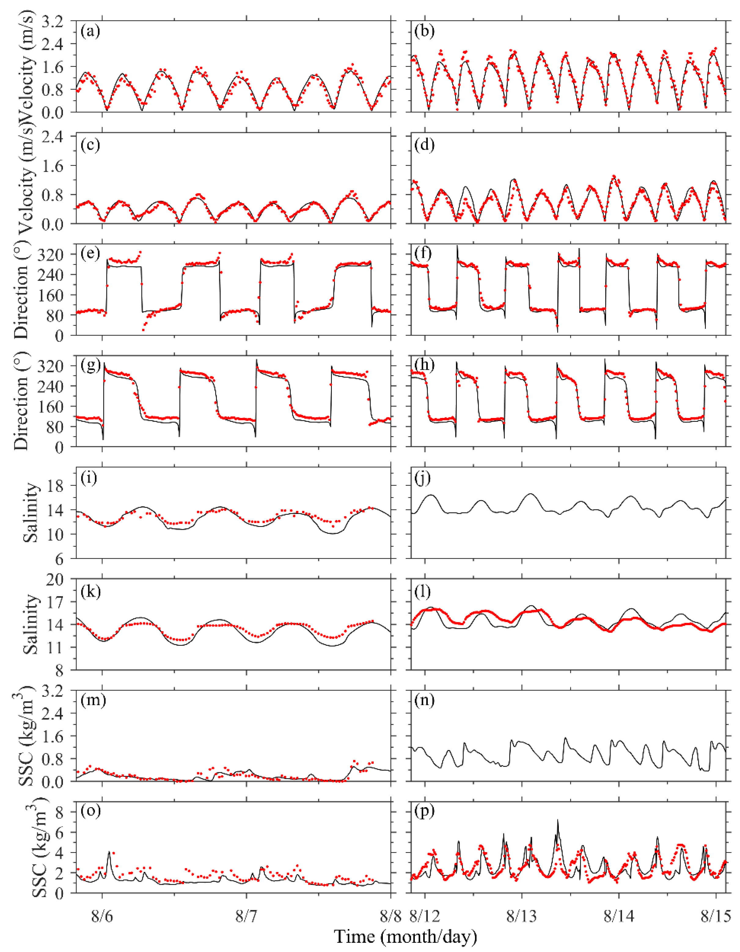
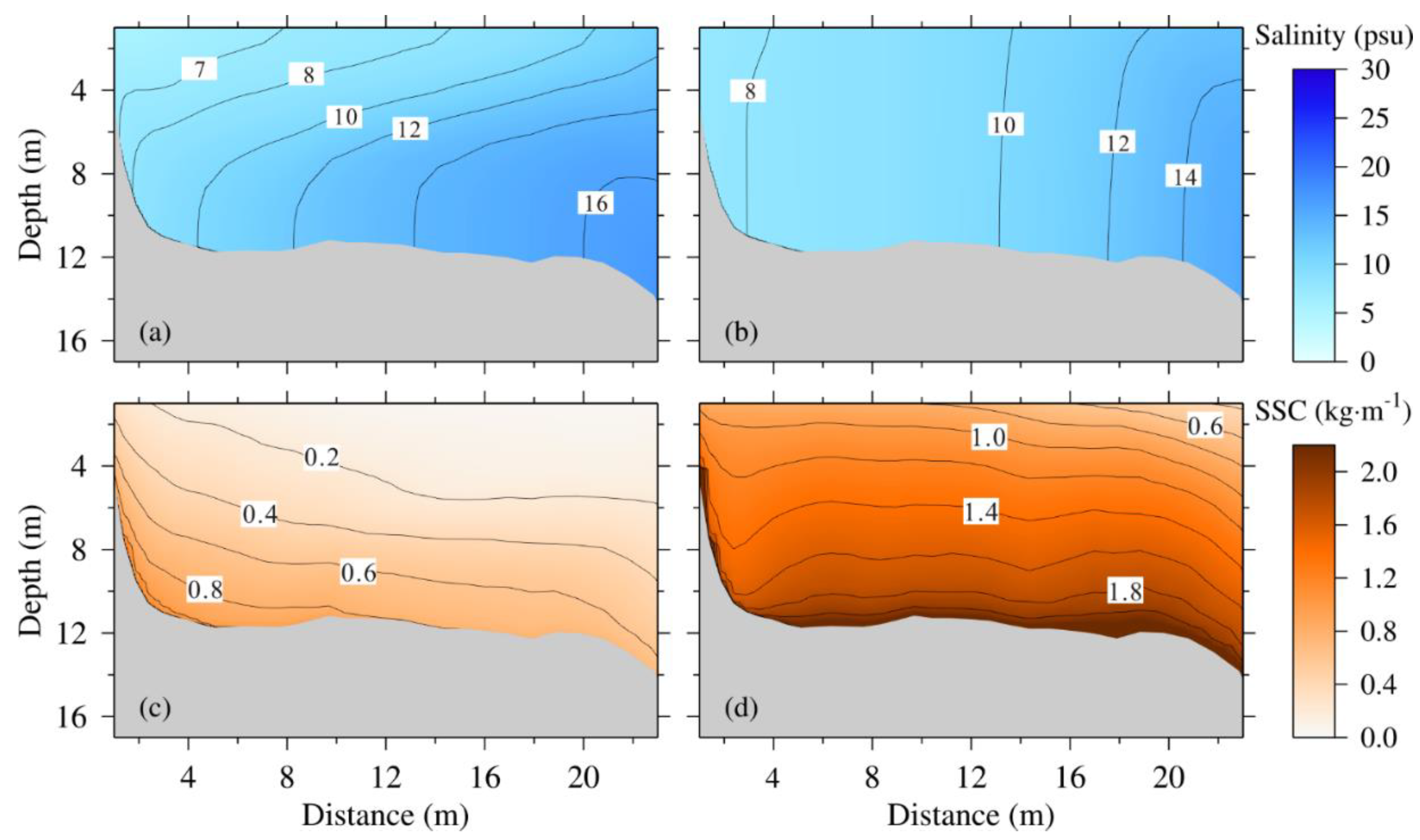
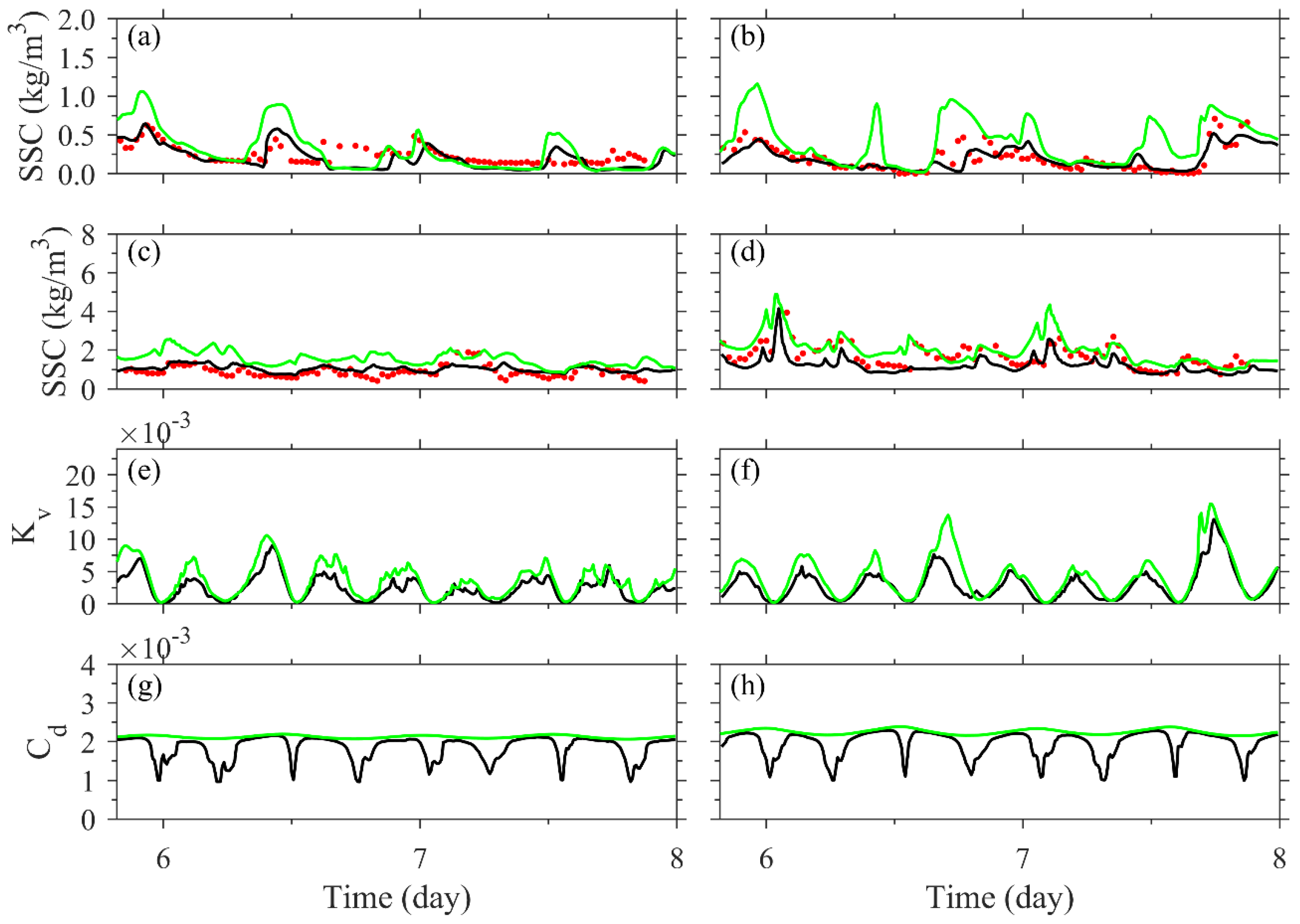
2.2. Model Validation

The numerical model has been extensively validated in terms of water level, current speed and direction, salinity, and SSC in the Changjiang Estuary and adjacent sea [39,44,77,78]. The model will be further validated in Hangzhou Bay. The following three skill assessments were used to quantify the validation: correlation coefficient (CC), root mean square error (RMSE), and skill score (SS) [79,80,81]:
CC   = ( X mod X mod ¯ ) ( X obs X obs ¯ ) [ ( X mod   X mod ¯ ) 2 ( X obs   X obs ¯ ) 2 ] 1 2
SS   = 1 ( X mod   X obs ) 2 ( | X mod   X mod ¯ | + | X obs   X obs ¯ | ) 2
RMSE   = ( X mod   X obs ) 2 N
where X is the variable and X ¯ is the time-averaged value. The performance levels of modeled results and observed results were evaluated by SS: >0.65 excellent; 0.65–0.5 very good; 0.5–0.2 good; <0.2 poor.
The in situ current velocity, salinity, and SSC at the anchored ship stations located at Hangzhou Bay (Figure 1) in August 2018 were used to validate the model. The model was cold started on 1 July 2018 and ran for 62 days. The real-time river discharge at Datong hydrologic station and Fuchunjiang hydroelectric power station, and the wind field data from ECMWF were downloaded to drive the model.
Comparisons of the modeled surface and bottom current velocities, salinity, and SSC with the observed data are shown in Figure 4 and Figure 5. There were higher values of correlation coefficients (CC), root-mean-square error (RMSE), and skill scores (SS) (Table 2). In particular, the skill score of the SSC reached more than 0.6, and some of them were above 0.75, indicating that the simulation results are very good. Therefore, the model successfully captured the variation processes of the water current, salinity, and SSC, and can be used to study the dynamics and SSC in Hangzhou Bay.
Due to the lack of observation data in winter, the SSC retrieved by satellite images was used for validation in this paper, which can also supplement the situation of spatial distribution. The SSC was retrieved from three cloudless or less cloudless GOCI satellite images downloaded from http://kosc.kiost.ac.kr/index.nm (accessed on 25 November 2021) in winter as compared with the simulated SSC in the surface layer. The SSC inversion algorithm proposed by Shen, et al. [82] for highly turbid waters was arithmetically expressed as follows:
SSC = 2   ·   α   ·   R r s β   ·   ( α R r s ) 2
where Rrs is the remote sensing reflectance obtained from atmospheric correction; and α and β are empirical and wavelength-dependent coefficients. For specific values, see Shen, et al. [83].
Comparisons of SSC derived from the GOCI with simulated SSC fields are shown in Figure 6. The high SSC in Hangzhou Bay was located in Andong tidal flat on the south coast and Nanhui tidal flat on the north coast of the bay. The surface SSC simulated by the model was consistent with the satellite inversion of SSC at the corresponding time. Therefore, the three-dimensional numerical model could successfully simulate the distribution of SSC in Hangzhou Bay.

3. Results

The model was cold started from 1 July to 31 August and 1 January to 28 February with climatological wind (monthly mean of 1979–2018) and river discharge (monthly mean of 1950–2018) for summer and winter, respectively, and the subtidal results of the last half month were output for analysis.

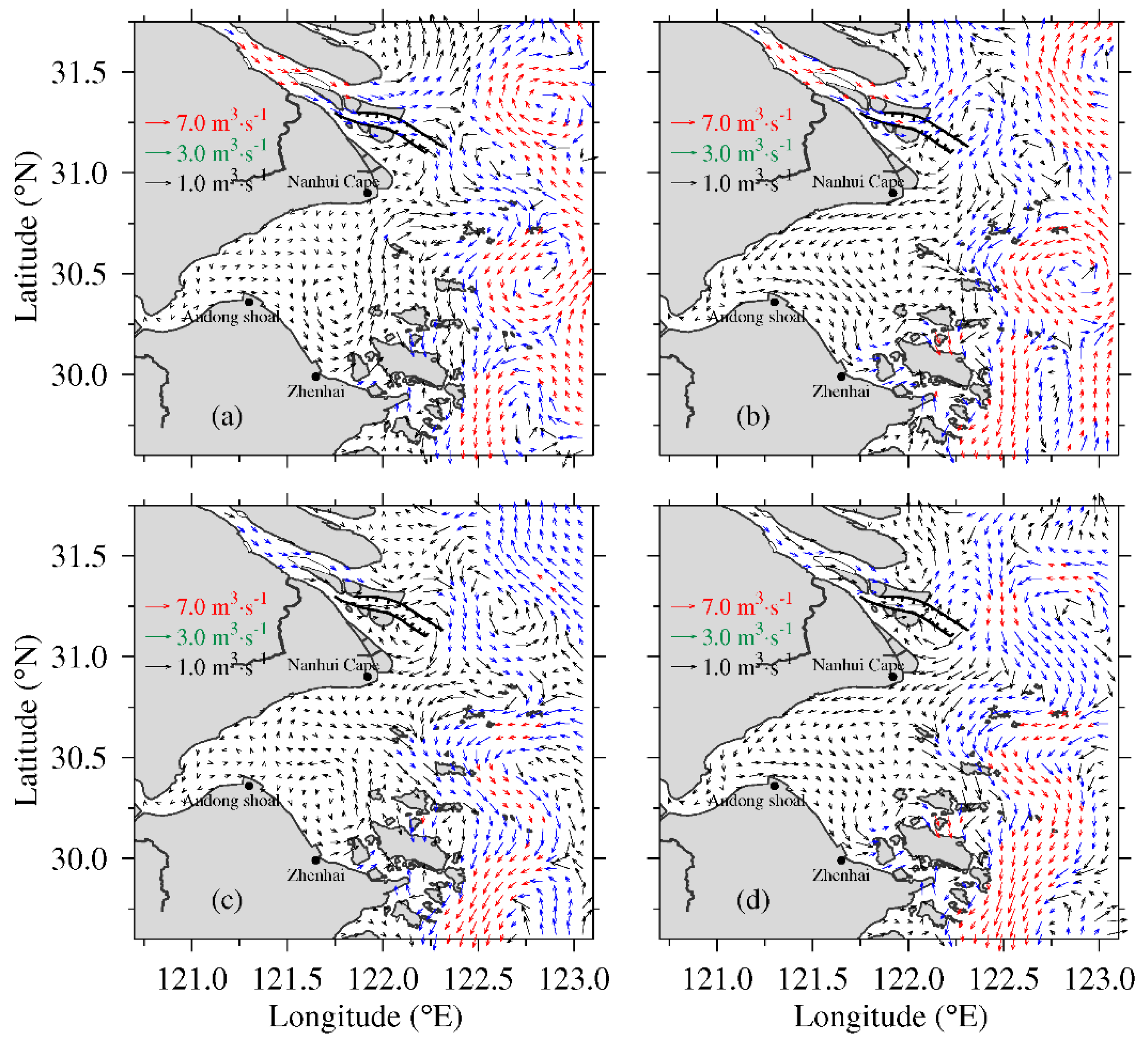
3.1. Water Flux Transport

The residual water level in the inner Changjiang mouth and Hangzhou Bay is higher in summer than in winter because the river discharge is much larger in summer than in winter, and it is higher in spring tide than in neap tide (Figure 7). The higher residual water level at the head of Hangzhou Bay is caused by the Qiantang River discharge. The residual water level near Nanhui Cape is higher on the north side near the south passage of the Changjiang Estuary than that on the south side and is also higher along the north coast of Hangzhou Bay than that along the south coast, which is caused by the large amount of river discharge from the Changjiang River into the bay.
Hangzhou Bay is a shallow bay and has a large tidal range; the residual current cannot properly reflect the net water transport. Therefore, the residual unit width water flux (RUWF) was used to reflect the water transport, which is defined as
RUWF = 1 T 0 T h 1 h 2 V d z d t
where V is the instantaneous horizontal velocity vector; h1 and h2 are the depth at the lower and upper boundaries of a certain layer; T is one or more complete cycles; and unit width here means 1 m. In this study, six semidiurnal tidal cycles ( ~ 3d) were used as an averaging time window to remove the semidiurnal and diurnal tidal signals during spring and neap tide. The thickness of the surface and bottom layers was one-tenth of the total water depth over the tidal cycle.
Figure 8 shows the distribution of RUWF and salinity in the surface and bottom layer during spring and neap tide in summer. The inner RUWF of the Changjiang mouth flows toward the sea across the water level contours, reflecting a nongeostrophic flow due to the small spatial scale. The surface RUWF flows along the water level contours in the outer Changjiang mouth and in the outer Hangzhou Bay, reflecting a quasi-geostrophic flow due to relatively large spatial scale. Off the Changjiang mouth, part of the surface RUWF flows northeastward in the neap tide under the force of southerly wind, flows northward east of Chongming Island in the spring tide due to tidal pumping and Stokes transport [41], and another part flows southward along the salinity front and into Hangzhou Bay along the isolines, reflecting the Changjiang secondary plume crossing Nanhui Cape [21]. In Hangzhou Bay, part of the surface RUWF from the Changjiang Estuary is transported directly to the Zhenhai area, and the other part is transported westward along the north coast, and then, it turns to the south coast and flows eastward to the Zhenhai area, which is consistent with the characteristic of the “north-landward and south-seaward” current pattern [6,26]. The surface pattern of RUWF is roughly consistent with the residual water level distribution, and more water is transported into the bay from the Changjiang Estuary in the spring tide than in the neap tide. In the bottom layer, the RUWF off the Changjiang mouth flows toward the estuary due to the strong baroclinic effect induced by the salinity front, and it is larger in the neap tide than in the spring tide. In Hangzhou Bay, the RUWF of Zhenhai is transported northward and is larger in the neap tide than in the spring tide. Near Nanhui Cape, the RUWF flows northward into the south passage of the Changjiang Estuary in the neap tide but flows westward into the bay from the adjacent sea rather than from the Changjiang Estuary in the spring tide, where the salinity front is stronger in the neap tide than in the spring tide. West of the Andong shoal, the pattern of bottom RUWF is similar to the surface RUWF, and it is still larger in the spring tide than in the neap tide.
Figure 9 shows the distribution of RUWF and salinity in the surface and bottom layer during the spring and neap tides in the winter. The RUWF in the inner Changjiang mouth is smaller than that in the summer due to the smaller river discharge. Under the force of northerly winds, the surface water from the Changjiang Estuary expands southward along the salinity front of the river mouth, and part of the surface water flows into Hangzhou Bay, which is stronger in the spring tide than in neap tide, and the distance of westward flow in the winter is shorter than that in the summer. In the bottom layer, the RUWF flows northward from the Zhenhai area to Nanhui Cape, which is the same as that in the summer but is much smaller due to the weaker salinity gradient. In the middle of the bay, the RUWF flows westward at the Andong shoal during the neap tide, and during the spring tide, the RUWF is similar to that in the summer, although somewhat smaller.
The distribution of RUWF in the whole layer during the spring and neap tides in the summer and winter is shown in Figure 10. In the summer, the water from the Changjiang Estuary is mainly transported from the north channel into the sea, and then, it flows northeast-northward in the neap tide and northward and southward in the spring tide. In Hangzhou Bay, the RUWF flows northward at the mouth and has a cyclonic eddy north of Zhenhai, and it flows westward along the north coast and eastward along the south coast with small values in the middle and western parts of the bay during the neap tide. More water from the Changjiang Estuary is transported into Hangzhou Bay during the spring tide, and it flows westward along the north coast; then, it flows eastward along the south coast, forming a distinct horizontal circulation that is “north-landward and south-seaward” in the bay. In the winter, the water from the Changjiang Estuary is transported southward under the force of the northerly wind, and a small part flows into Hangzhou Bay. In Hangzhou Bay, the RUWF is weak and still has a cyclonic eddy north of Zhenhai in the neap tide, and during the spring tide, the pattern is very similar to that in the summer, only the magnitude is slightly smaller.

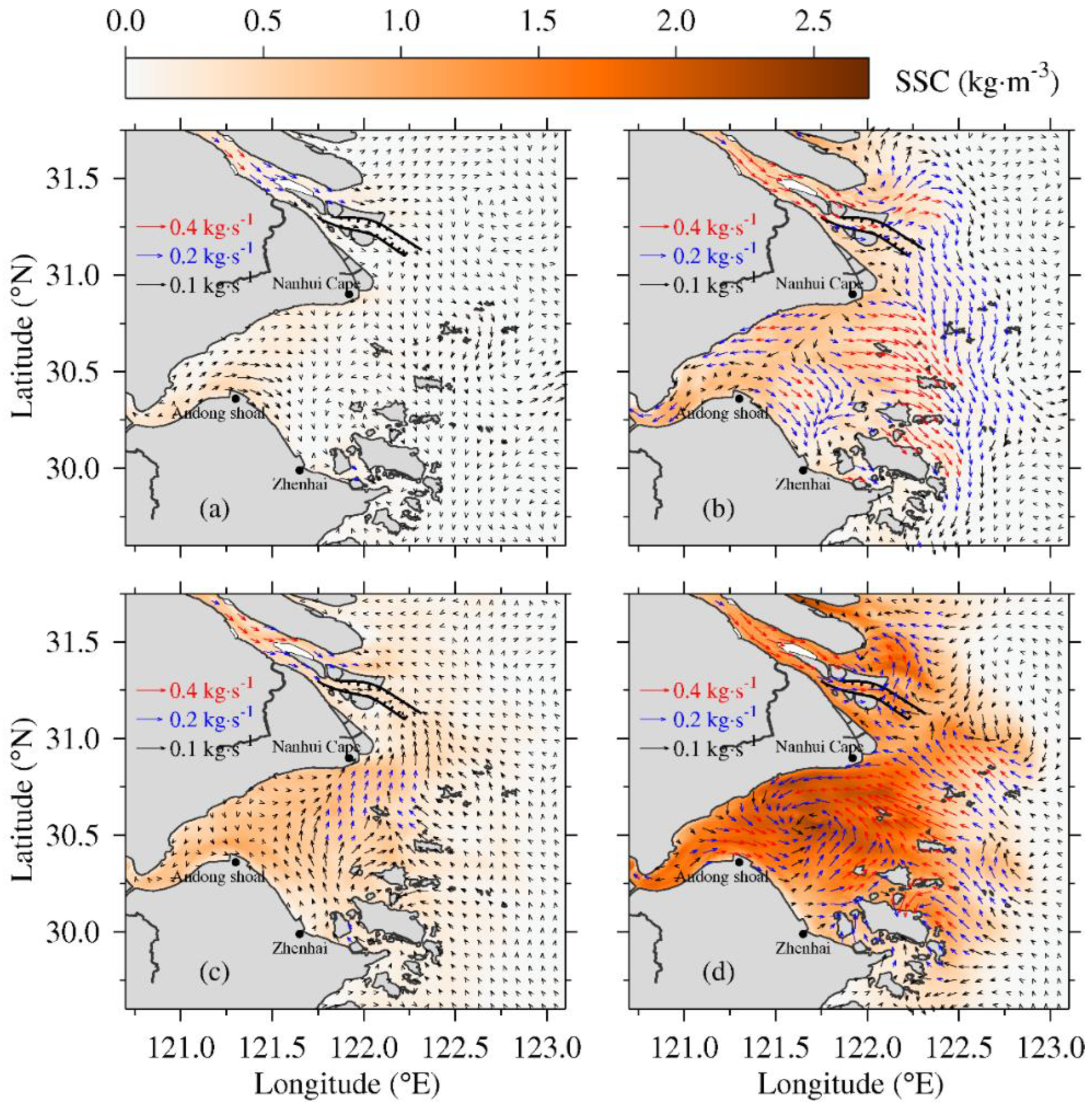
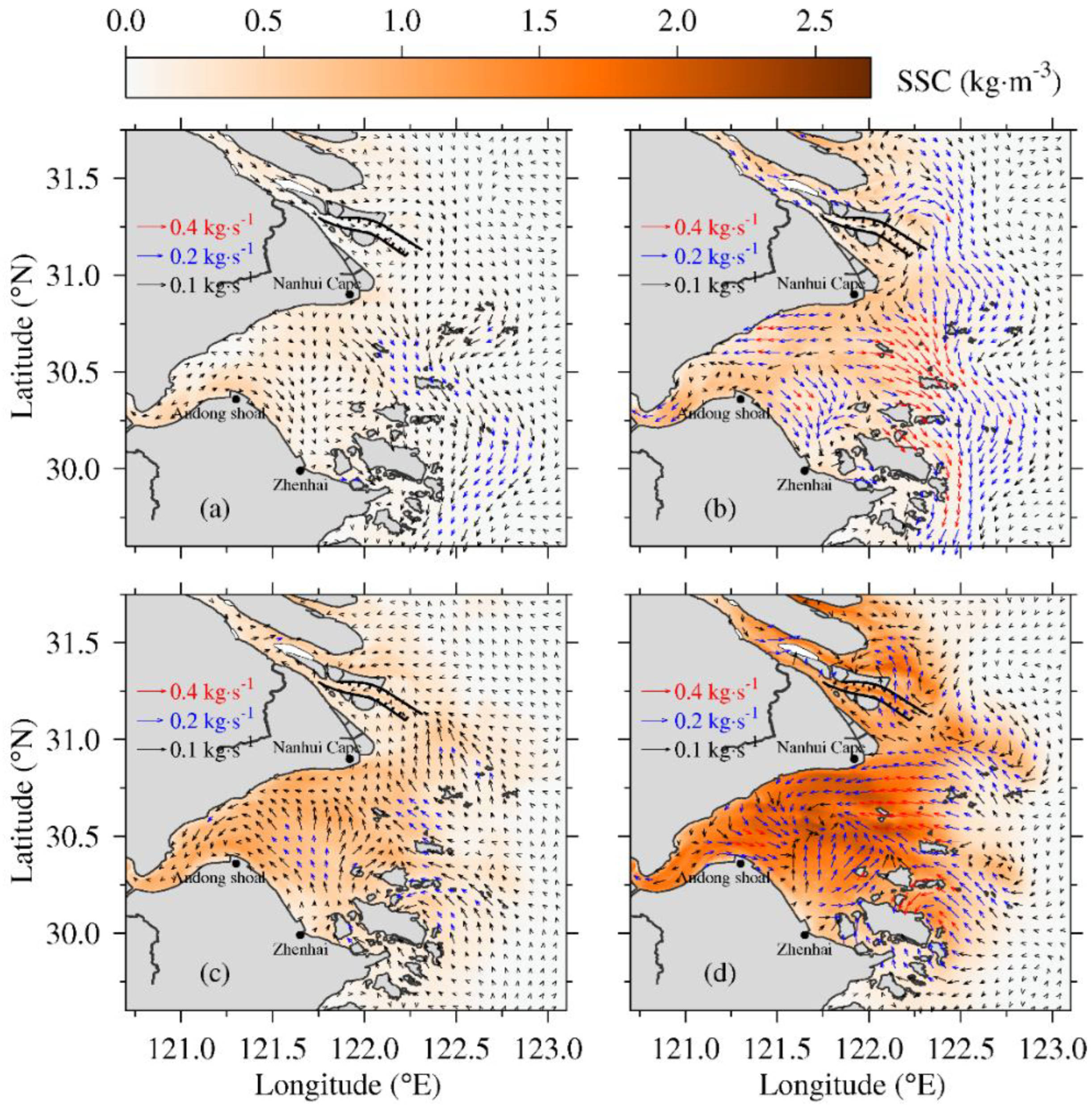
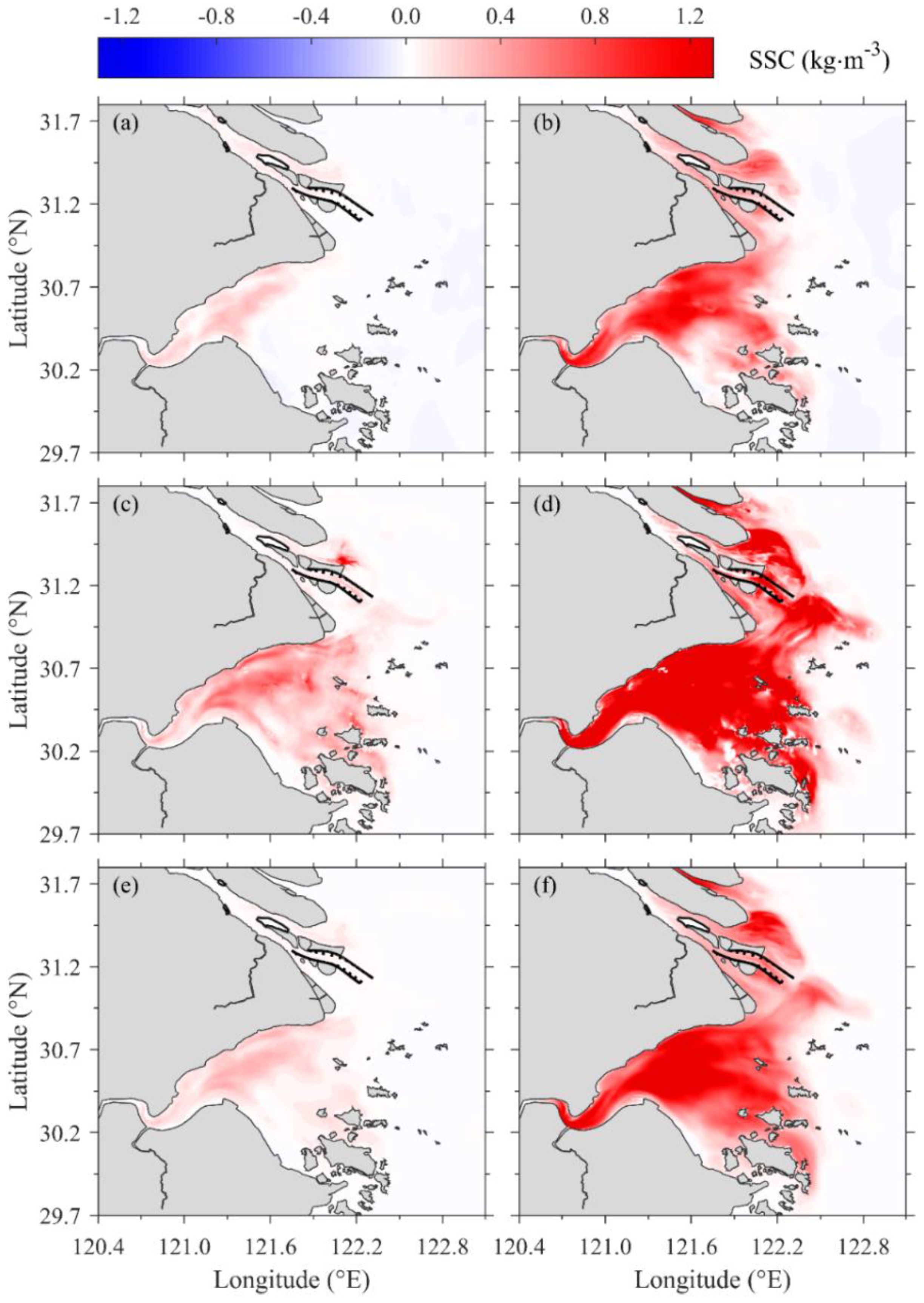
3.2. Suspended Sediment Transport

In this paper, the residual unit width sediment flux (RUSF) was used to reflect the transport of suspended sediment.
RUSF   = 1 T 0 T h 1 h 2 V · C · d z d t
The distribution of RUSF and SSC in the surface and bottom layer during the spring and neap tide in the summer is shown in Figure 11. In addition to the sediment subsidence and diffusion in the water column and suspension on the seabed, the sediment transport is mainly controlled by the horizontal sediment advection; therefore, the pattern of RUSF is similar to that of the water flux transport. During the neap tide, the surface RUSF and SSC are small in Hangzhou Bay. The sediment is transported southward from the Changjiang Estuary to the Zhenhai area with a small magnitude, and it is transported seaward in the middle and western part of the bay. In the bottom layer, the SSC is approximately 1.0 kg·m−3, which is much higher than that in the surface layer; the sediment is transported northward from the Zhenhai area to Nanhui Cape and Changjiang mouth with a larger magnitude of approximately 0.1 kg·s−1 induced by the strong estuarine baroclinic effect, and it is transported westward along the north coast and eastward along the south coast in the western area of the bay; in the Andong tidal flat, the sediment is transported from both the west and east sides, resulting in higher SSC there.
During the spring tide, the surface and bottom SSC reaches 1.0 and 2.5 kg·m−3 on the north side of the central Hangzhou Bay, which is much larger than that in the neap tide, caused by the great suspension of bed sediment due to a strong tidal current in the spring tide. In the surface layer, the RUSF flows southward to the Zhenhai area and westward along the north coast of the bay from the Changjiang Estuary. In the bottom layer, the RUSF flows northwestward toward the Changjiang mouth off the mouth of Hangzhou Bay with a larger value of 0.3 kg·s−1, and it has a large cyclonic transport in Hangzhou Bay with a value of 0.25 kg·s−1. The sediment is transported eastward in the middle and western parts of the bay.
The distribution of RUSF and SSC in the surface and bottom layer during the neap and spring tide in the winter is shown in Figure 12. During the neap tide, the surface RUSF and SSC in Hangzhou Bay are similar to that in the summer; additionally, the SST is slightly larger, and the RUSF near Nanhui Cape in the bottom layer is weaker than that in the summer. During the spring tide, the surface sediment transport is similar to that in the summer. In the bottom layer, the sediment of the bay mouth is transported into the bay and Changjiang mouth; then, it is transported eastward in the middle and western areas of the bay and converges in the center of the bay, resulting in higher SSC there.
Figure 13 shows the RUSF in the whole layer during the spring and neap tide in the summer and winter. The suspended sediment exchange between the Changjiang Estuary and Hangzhou Bay has a significant variation during the neap and spring tide. The suspended sediment is transported from the Zhenhai area to the Changjiang mouth in the neap tide and from the Changjiang mouth into Hangzhou Bay westward along the north coast and eastward along the south coast in the spring tide. The magnitude of sediment transport is much larger in the spring tide than that in the neap tide. In the summer, the sediment is transported eastward in the middle of the bay with a value of approximately 0.10 kg·s−1, and it is transported westward along the north coast and eastward along the south coast in the area west of the bay in the neap tide. In the spring tide, the sediment is transported westward along the north coast and eastward along the south coast, forming a large cyclonic circulation in the whole bay, which is consistent with the pattern of “north-landward and south-seaward” in Hangzhou Bay [26].
In the winter, the suspended sediment in the middle of Hangzhou Bay is transported northward to the north coast, and then, the direction turns westward in the western area of the bay in the neap tide. In the spring tide, the pattern of RUSF in Hangzhou Bay is very similar to that in the summer. Off the bay mouth, the suspended sediment flows southward farther through the Zhoushan Islands, reinforced by the northerly winds, as confirmed by Liu et al. [19].

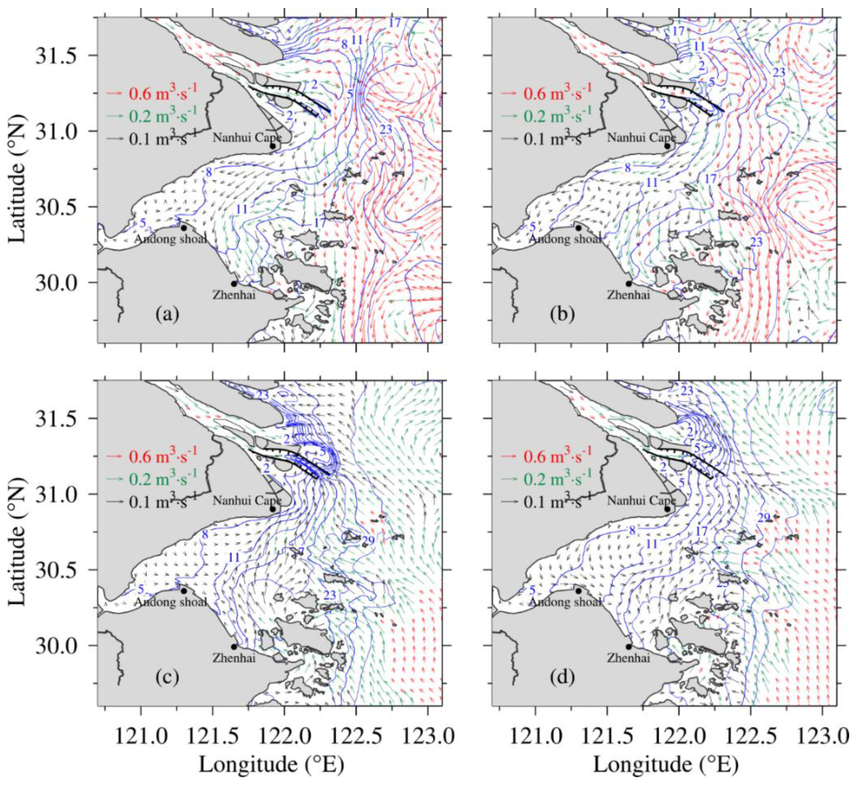
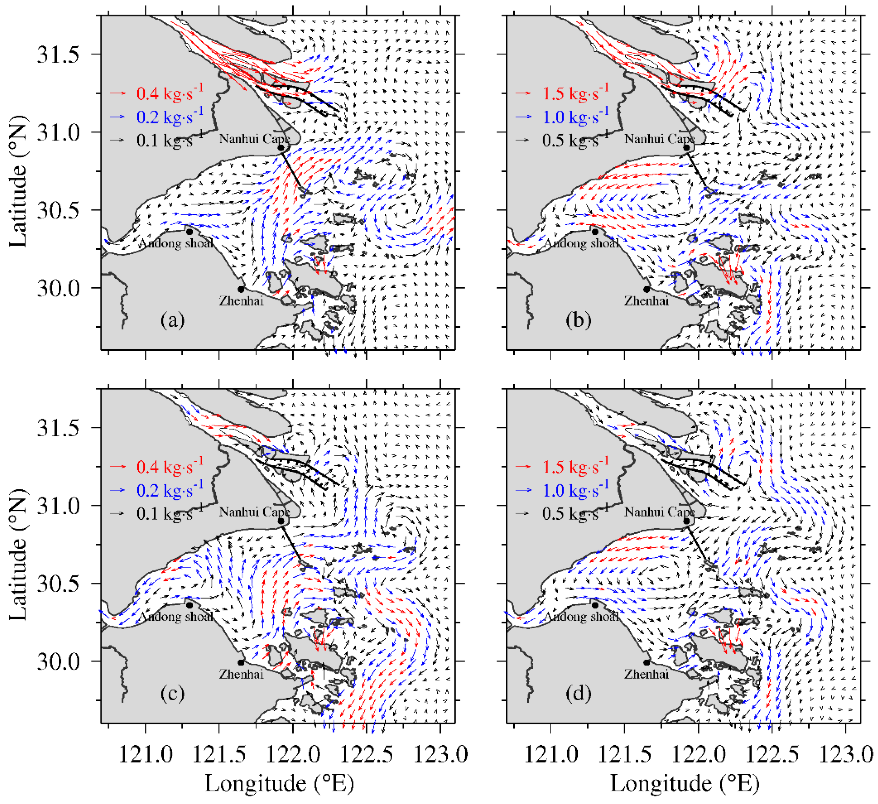
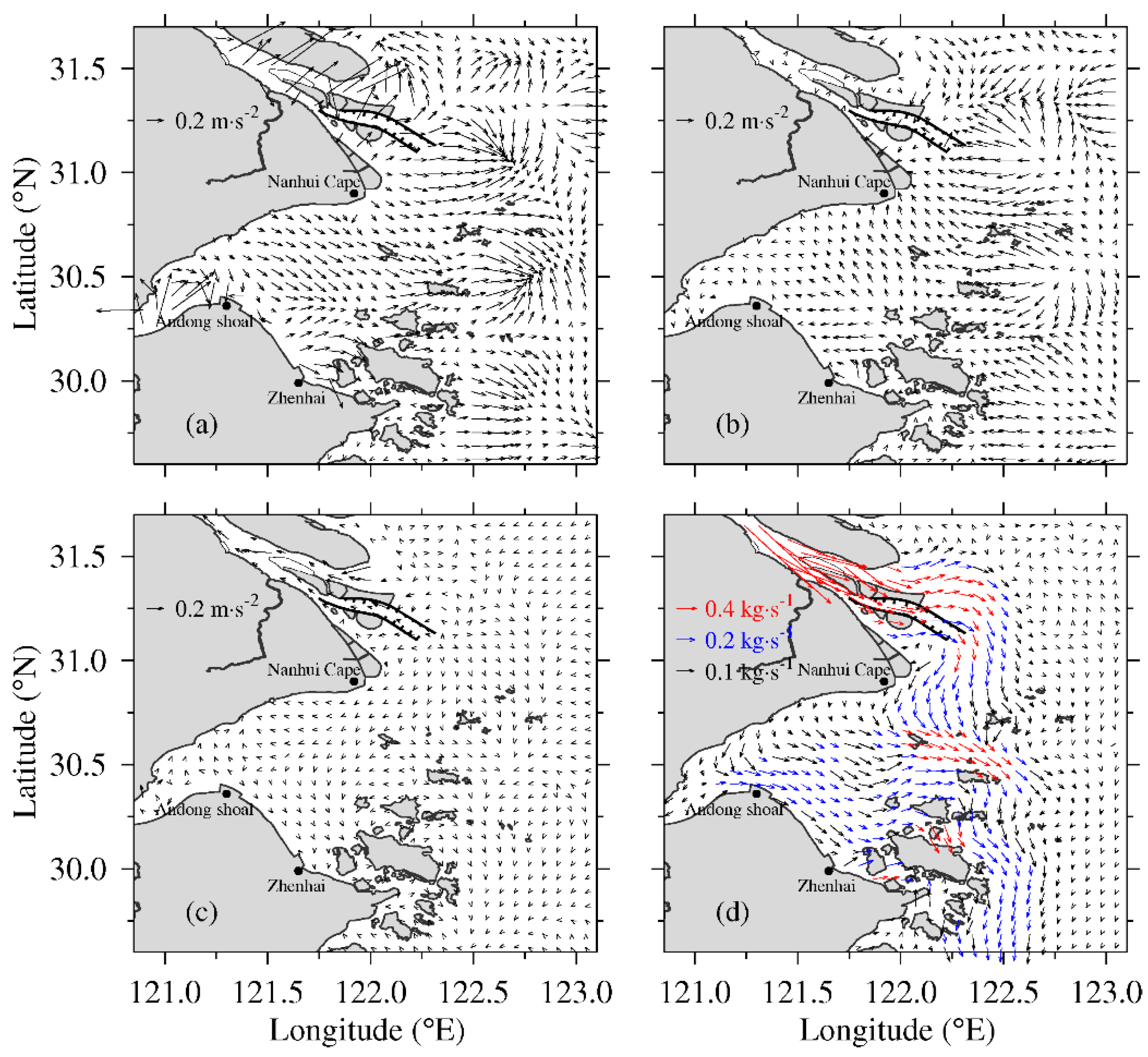
3.3. Water and Sediment Exchange Flux between the Changjiang Estuary and Hangzhou Bay

The results in Section 3.1 and Section 3.2 show that there is a water and sediment exchange between the Changjiang Estuary and Hangzhou Bay. To further quantify the water and sediment exchange, a section from Nanhui Cape to the Qiqu Archipelago section (NQ section) was selected (position indicated in Figure 1). Figure 14 shows the distribution of salinity and SSC across the NQ section in the summer. The surface salinity is lower, and the bottom salinity is higher during the neap tide. There is a stratification of salinity in the neap tide and vertical uniformity of salinity in the spring tide because the vertical mixing varies with the tide. The SSC during the spring tide is much larger than that during the neap tide because much more sediment on the seabed is suspended by the larger bottom-shear stress and then vertically diffused to the surface much stronger in the spring tide. The SSC in the surface layer is always lower than that in the bottom layer due to sediment settling.
The net transect water flux (NTWF) and the net transect sediment flux (NTSF) across a section were calculated as the following equations:
NTWF = 0 T H ζ 0 L V n d l d z d t
NTSF = 0 T H ζ 0 L C V n d l d z d t
where ζ is the surface level; L is the width of the transect; C is the SSC; V n is the velocity component normal to the transect; and T is six semidiurnal tidal cycles (~3d) during the spring or neap tide.
In the summer, the water and sediment transport flux across the NQ section are −2.91 × 10⁹ m3 and −4.16 × 10⁹ kg during the spring tide, and 4.29 × 10⁹ m3 and 2.44 × 10⁹ kg during the neap tide (Table 3), respectively, meaning that they are transported from the Changjiang Estuary into Hangzhou Bay in the spring tide, but they are transported from Hangzhou Bay into the Changjiang Estuary in the neap tide. In one month, the water and sediment transport flux across the section is from the Changjiang Estuary into Hangzhou Bay with values of −7.81 × 10⁹ m3 and −4.80 × 10⁹ kg, respectively.
In the winter, the water and sediment transport flux across the NQ section are −2.27 × 10⁹ m3 and −4.30 × 10⁹ kg during the spring tide, and −1.60 × 10⁸ m3 and 9.30 × 10⁸ kg during the neap tide, respectively, meaning that they are transported from the Changjiang Estuary into Hangzhou Bay in the spring tide. However, in the neap tide, the water transport flux is still from the Changjiang Estuary into Hangzhou Bay, but the sediment transport flux is from Hangzhou Bay into the Changjiang Estuary. This is because the SSC is much higher in the bottom layer than that in the surface layer and the RUWF in the bottom layer flows into the Changjiang Estuary (Figure 9c). In one month, the water and sediment transport flux across the section is from the Changjiang Estuary into Hangzhou Bay with values of −1.34 × 10¹⁰ m3 and −2.16 × 10¹⁰ kg, respectively. Much more water and sediment are transported across the section from the Changjiang Estuary into Hangzhou Bay in the winter than in the summer, which is consistent with the results of Bian, et al. [84] obtained by measured data.

4. Discussion

To discuss the dynamic mechanism of suspended sediment transport in Hangzhou Bay, two numerical experiments were set up in the case of the summer. Exp 1 is without turbidity-influenced stratification and bottom drag coefficient, and Exp 2 is without baroclinic pressure gradient force. Other dynamic factors are the same as the numerical simulation in Section 3, called the control experiment.

4.1. Effect of Turbidity-Influenced Stratification and Bottom Drag Coefficient on Suspended Sediment Transport

Hangzhou Bay is a highly turbid water body, which can affect the stratification in the water column. The turbidity-induced stratification, which is calculated by Formula (8), inhibits vertical eddy diffusivity. This results in the accumulation of sediment in the BBL, forming a fluid mud layer, which can cause a reduction in the bottom drag coefficient, shown by Formula (9). High-turbidity water can enhance vertical stratification and reduce vertical mixing and the bottom drag coefficient. The temporal variation in the modeled surface and bottom SSC, vertically averaged eddy diffusivity, and bottom drag coefficient at measured sites A and B (locations shown in Figure 1) with and without turbidity-influenced stratification and the bottom drag coefficient are shown in Figure 15. Considering the real case with turbidity-influenced stratification and the bottom drag coefficient, the surface and bottom SSC, vertical eddy diffusivity, and bottom drag coefficient greatly decrease, showing that the modeled surface and bottom SSTs are much more consistent with the observed values. At measured sites A and B, considering the turbidity-influenced stratification and bottom drag coefficient, the vertical eddy diffusivity (Kv) decreases by 50.7% and 45.3%, and the bottom drag coefficient (Cd) decreases by 15.4% and 14.8%, respectively, compared with that without the turbidity-influenced stratification and bottom drag coefficient, resulting in the surface SSC decreasing by 47.5% and 119.2%, and the bottom SSC decreasing by 49.0% and 64.7%, respectively. Therefore, the turbidity-influenced stratification and bottom drag coefficient have significant impacts on sediment suspension in the seabed and vertical diffusion.
The SSC difference between Exp 1 and the control experiment in the surface layer, bottom layer, and whole layer during the neap tide and spring tide are shown in Figure 16. Without the turbidity-influenced stratification and bottom drag coefficient, the SSC distinctly increases due to the larger bottom stress and stronger vertical mixing. The difference in SSC is much larger in the spring tide than in the neap tide because more sediment is suspended on the seabed and vertically diffused in the spring tide.

4.2. Effect of Baroclinic Pressure Gradient Force on Suspended Sediment Transport

The above results show that the surface RUWF on the south side of Nanhui Cape is in the opposite direction to the bottom RUWF during the neap tide; that is, the bottom RUWF flows to the south passage, so this is the RUSF. The sediment flux across the NQ section indicates that the NTSF flows into Hangzhou Bay during the spring tide in the summer and winter, and the NTSF flows into the Changjiang Estuary during the neap tide in the summer and winter. Why is there such a large difference in sediment transport between the spring and neap tide? Next, the main terms in the Navier-Stokes momentum equations are analyzed to discuss the dynamic mechanism.
During the neap tide in the summer, the tidally averaged barotropic pressure gradient force is seaward off the Changjiang mouth and southeastward in Hangzhou Bay (Figure 17a), corresponding to the distribution of residual water level (Figure 7a). The tidally and vertically averaged baroclinic pressure gradient force is southward off the Changjiang mouth and is westward or northwestward in most of the sea areas of Hangzhou Bay, and northward in the south side of Nanhui Cape (Figure 17b), corresponding to the distribution of salinity (Figure 8a,c). Compared with the barotropic pressure gradient force and baroclinic pressure gradient force, the vertical turbulent viscous force, i.e., the resultant force of wind stress and bottom friction is small. Not considering the baroclinic pressure gradient force, the RUSF in the whole layer flows into Hangzhou Bay near Nanhui Cape and flows southeastward in the middle and eastern parts of the bay, which is quite different from the sediment transport with the baroclinic pressure gradient force (Figure 13a), that flows northward from Zhenhai to Nanhui Cape, meaning that only the baroclinic pressure gradient force drives the sediment transport northward during the neap tide.
In the spring tide in the summer, the baroclinic pressure gradient force is still southward off the Changjiang mouth. In Hangzhou Bay, the baroclinic pressure gradient force is similar to the neap tide and is more northwestward in the south side of Nanhui Cape than that in the neap tide (Figure 18b), but its magnitude is smaller than that in the neap tide. The barotropic pressure gradient force is significantly larger than the baroclinic pressure gradient force (Figure 18a, the scale is 0.4 m·s−2, larger than that in Figure 18b), resulting in the RUSF in the whole layer flowing westward along the north coast and eastward along the south coast in the bay with a larger magnitude (Figure 18d). Not considering the baroclinic pressure gradient force, the RUSF in the whole layer is similar to the RUSF considering the baroclinic pressure gradient force in the control experiment (Figure 13b). Therefore, the water and sediment transported from the Changjiang Estuary into Hangzhou Bay during the spring tide are mainly driven by the barotropic pressure gradient force, and they are transported from Hangzhou Bay into the Changjiang Estuary during the neap tide in the summer, which is mainly driven by the baroclinic pressure gradient force.

5. Conclusions

With the combined consideration of the settlement, erosion and deposition, flocculation of sediment, waves, turbidity-influenced stratification, and bottom drag coefficient, a high-resolution three-dimensional sediment numerical model is established to simulate and analyze the water and sediment transport in Hangzhou Bay. Model validation shows that the skill score of the SSC has reached more than 0.6, indicating the model can successfully simulate the SSC in Hangzhou Bay. The conclusions are summarized as follows.
In the summer, the surface RUWF from the Changjiang Estuary near Nanhui Cape flows westward along the coast, in which the major part of it flows southward to the Zhenhai area, and a small part of it flows further westward along the north coast. Then, it turns to the south coast and flows eastward, forming the water transport pattern of north-landward and south-seaward in the surface layer, which is stronger in the spring tide than in the neap tide. In the bottom layer, the RUWF near Zhenhai flows northward to Nanhui Cape in the neap tide and to the south passage of the Changjiang Estuary. In the middle and western parts of the bay, the RUWF has the same pattern as the surface water transport, which is stronger in the spring tide than in the neap tide and weaker in the bottom layer than in the surface layer. The RUSF pattern is roughly similar to the water flux transport. During the spring tide, the SSC is much larger than in neap tide and larger in the bottom layer than in the surface layer. The water and sediment transport flux across the NQ section are from the Changjiang Estuary into Hangzhou Bay during the spring tide, but from Hangzhou Bay into the Changjiang Estuary during the neap tide.
In the winter, the RUWF, RUSF, and SSC in Hangzhou Bay are similar to those in the summer; the distance of the surface water transport westward along the north coast is shorter than that in the summer, and the magnitude of the bottom RUWF is smaller than that in the summer due to the weaker salinity gradient. The SSC is slightly larger, and the bottom RUSF near Nanhui Cape is weaker than that in the summer during the neap tide. The water and sediment transport flux across the NQ section are from the Changjiang Estuary into Hangzhou Bay during the spring tide, and during the neap tide, the water transport flux is still from the Changjiang Estuary into Hangzhou Bay, but the sediment transport flux is from Hangzhou Bay into the Changjiang Estuary because the SSC is much higher in the bottom layer than in the surface layer. Finally, the NTSF flows into the Changjiang Estuary.
The sensitivity numerical experiments indicated that the turbidity-influenced stratification and bottom drag coefficient have significant impacts on sediment suspension for the seabed and vertical diffusion, and the high-turbidity water enhances vertical stratification and reduces vertical mixing and the bottom drag coefficient, resulting in the modeled SSC being much more consistent with the observed value. The reason why the water and sediment are transported from the Changjiang Estuary into Hangzhou Bay during the spring tide in the winter and summer is mainly that the offshore barotropic pressure gradient force is larger than the onshore baroclinic pressure gradient force. Furthermore, the reason why the sediment is transported from Hangzhou Bay into the Changjiang Estuary during the neap tide in the summer and winter is mainly because the baroclinic pressure gradient force is larger than the barotropic pressure gradient force.
Although the model is now validated, it is still an approximation of reality. Additionally, in the field, additional mechanisms for residual transport may exist. For example, variations in freshwater discharge, sediment load, wind speed and direction, wave forcing, and water level at the sea boundary may strongly influence residual transport. To further investigate this, additional sensitivity numerical experiments on forcing factors will be set up in future studies.

Author Contributions

Conceptualization, J.H. and J.Z.; methodology, J.H. and J.Z.; software, J.H. and J.Z.; validation, J.H.; formal analysis, J.H. and R.Y.; investigation, J.H. and R.Y.; resources, J.H. and J.Z.; data curation, J.H. and R.Y.; writing—original draft preparation, J.H.; writing—review and editing, J.Z.; visualization, J.H. and R.Y.; supervision, J.Z.; project administration, J.Z.; funding acquisition, J.Z. All authors have read and agreed to the published version of the manuscript.

Funding

This work was supported by the Science and Technology Commission of Shanghai Municipality (21JC1402500).

Institutional Review Board Statement

Not applicable.

Informed Consent Statement

Not applicable.

Acknowledgments

We also acknowledge the anonymous reviewers for their valuable comments and suggestions.

Conflicts of Interest

The authors declare no conflict of interest.

References

  1. Fang, H.W.; Huang, L.; Wang, J.Y.; He, G.J.; Reible, D. Environmental assessment of heavy metal transport and transformation in the Hangzhou Bay, China. J. Hazard. Mater. 2016, 302, 447–457. [Google Scholar] [CrossRef] [PubMed]
  2. Huang, Y.G.; Yang, H.F.; Jia, J.J.; Li, P.; Zhang, W.X.; Wang, Y.P.; Ding, Y.F.; Dai, Z.J.; Shi, B.W.; Yang, S.L. Declines in suspended sediment concentration and their geomorphological and biological impacts in the Yangtze River Estuary and adjacent sea. Estuar. Coast. Shelf Sci. 2022, 265, 107708. [Google Scholar] [CrossRef]
  3. Zhao, X.; Wang, S.S.; Pan, C.H.; Mu, J.B.; Li, L.W.; Zhu, Y.Z. Distribution characteristics and ecological risk assessment of nutrients in sediment particles in Hangzhou Bay, China. In Proceedings of the IOP Conference Series: Earth and Environmental Science, Taiwan, China, 17–21 July 2018; p. 012079. [Google Scholar]
  4. Liu, G.F.; Zhu, J.R.; Wang, Y.Y.; Wu, H.; Wu, J.X. Tripod measured residual currents and sediment flux: Impacts on the silting of the Deepwater Navigation Channel in the Changjiang Estuary. Estuar. Coast. Shelf Sci. 2011, 93, 192–201. [Google Scholar] [CrossRef]
  5. Zhu, L.; He, Q.; Shen, J.; Wang, Y. The influence of human activities on morphodynamics and alteration of sediment source and sink in the Changjiang Estuary. Geomorphology 2016, 273, 52–62. [Google Scholar] [CrossRef]
  6. Song, Z.K.; Shi, W.Y.; Zhang, J.B.; Hu, H.; Zhang, F.; Xu, X. Transport Mechanism of Suspended Sediments and Migration Trends of Sediments in the Central Hangzhou Bay. Water 2020, 12, 2189. [Google Scholar] [CrossRef]
  7. Xie, D.F.; Pan, C.H.; Wu, X.G.; Gao, S.; Wang, Z.B. Local human activities overwhelm decreased sediment supply from the Changjiang River: Continued rapid accumulation in the Hangzhou Bay-Qiantang Estuary system. Mar. Geol. 2017, 392, 66–77. [Google Scholar] [CrossRef]
  8. Yang, S.L.; Zhang, J.M.; Zhu, J.; Smith, J.P.; Dai, S.B.; Gao, A.; Li, P. Impact of dams on Yangtze River sediment supply to the sea and delta intertidal wetland response. J. Geophys. Res. Earth Surf. 2005, 110. [Google Scholar] [CrossRef]
  9. Zhu, B.Y.; Li, Y.T.; Yu, W.J.; Sun, Z.H.; Deng, J.Y.; Chai, Y.F.; Zhang, C.C. An analysis of the processes and trends of changes in Yangtze River water and sediment fluxes into the ocean. Resour. Environ. Yangtze Basin 2019, 28, 2980–2991, (In Chinese with English Abstract). [Google Scholar]
  10. Cheng, L.; Jueyi, S.; Yun, H.; Hirshfield, F. Changes in runoff and sediment load from major Chinese rivers to the Pacific Ocean over the period 1955–2010. Int. J. Sediment Res. 2013, 28, 486–495. [Google Scholar]
  11. Chen, S.L. Seasonal, neap-spring variation of sediment concentration in the joint area between Yangtze Estuary and Hangzhou Bay. Sci. China Ser. B Chem. 2001, 44, 57–62. [Google Scholar] [CrossRef]
  12. Dai, Z.J.; Chu, A.; Li, W.H.; Li, J.F.; Wu, H.L. Has suspended sediment concentration near the mouth bar of the Yangtze (Changjiang) Estuary been declining in recent years? J. Coast. Res. 2013, 29, 809–818. [Google Scholar] [CrossRef]
  13. Li, P.; Yang, S.L.; Milliman, J.D.; Xu, K.H.; Qin, W.H.; Wu, C.S.; Chen, Y.P.; Shi, B.W. Spatial, temporal, and human-induced variations in suspended sediment concentration in the surface waters of the Yangtze Estuary and adjacent coastal areas. Estuaries Coasts 2012, 35, 1316–1327. [Google Scholar] [CrossRef] [Green Version]
  14. Luo, W.; Shen, F.; He, Q.; Cao, F.; Zhao, H.Y.; Li, M.Y. Changes in suspended sediments in the Yangtze River Estuary from 1984 to 2020: Responses to basin and estuarine engineering constructions. Sci. Total Environ. 2022, 805, 150381. [Google Scholar] [CrossRef]
  15. Alexander, C.R.; DeMaster, D.J.; Nittrouer, C.A. Sediment accumulation in a modern epicontinental-shelf setting: The Yellow Sea. Mar. Geol. 1991, 98, 51–72. [Google Scholar] [CrossRef]
  16. DeMaster, D.J.; McKee, B.A.; Nittrouer, C.A.; Jiangchu, Q.; Guodong, C. Rates of sediment accumulation and particle reworking based on radiochemical measurements from continental shelf deposits in the East China Sea. Cont. Shelf Res. 1985, 4, 143–158. [Google Scholar] [CrossRef]
  17. Guo, Z.G.; Yang, Z.S.; Fan, D.J.; Pan, Y.J. Seasonal sedimentary effect on the Changjiang Estuary mud area. Acta Geogr. Sin. 2003, 58, 591–597, (In Chinese with English Abstract). [Google Scholar]
  18. Sternberg, R.; Larsen, L.; Miao, Y. Tidally driven sediment transport on the East China Sea continental shelf. Cont. Shelf Res. 1985, 4, 105–120. [Google Scholar] [CrossRef]
  19. Liu, J.P.; Xu, K.H.; Li, A.C.; Milliman, J.D.; Velozzi, D.M.; Xiao, S.B.; Yang, Z.S. Flux and fate of Yangtze River sediment delivered to the East China Sea. Geomorphology 2007, 85, 208–224. [Google Scholar] [CrossRef]
  20. Cao, P.K.; Gu, G.C.; Dong, Y.F.; Hu, F.X. Basic characteristics of sediment transport in Hangzhou Bay. J. East China Norm. Univ. (Nat. Sci.) 1985, 3, 75–84, (In Chinese with English Abstract). [Google Scholar]
  21. Su, J.L.; Wang, K.S. Changjiang river plume and suspended sediment transport in Hangzhou Bay. Cont. Shelf Res. 1989, 9, 93–111. [Google Scholar]
  22. Xie, D.F.; Pan, C.H.; Wu, X.G.; Gao, S.; Wang, Z.B. The variations of sediment transport patterns in the outer C hangjiang E stuary and H angzhou B ay over the last 30 years. J. Geophys. Res. Ocean. 2017, 122, 2999–3020. [Google Scholar] [CrossRef]
  23. Dai, Z.J.; Liu, J.T.; Xie, H.L.; Shi, W.Y. Sedimentation in the outer Hangzhou Bay, China: The influence of Changjiang sediment load. J. Coast. Res. 2014, 30, 1218–1225. [Google Scholar] [CrossRef]
  24. Wang, B.C.; Eisma, D. Supply and deposition of sediment along the north bank of Hangzhou Bay, China. Neth. J. Sea Res. 1990, 25, 377–390. [Google Scholar] [CrossRef]
  25. Chen, J.Y.; Liu, C.Z.; Zhang, C.L.; Walker, H.J. Geomorphological development and sedimentation in Qiantang Estuary and Hangzhou Bay. J. Coast. Res. 1990, 6, 559–572. [Google Scholar]
  26. Xie, D.F.; Wang, Z.B.; Gao, S.; De Vriend, H.J. Modeling the tidal channel morphodynamics in a macro-tidal embayment, Hangzhou Bay, China. Cont. Shelf Res. 2009, 29, 1757–1767. [Google Scholar] [CrossRef]
  27. Du, P.J.; Ding, P.X.; Hu, K.L. Simulation of three-dimensional cohesive sediment transport in Hangzhou Bay, China. Acta Oceanol. Sin. 2010, 29, 98–106. [Google Scholar] [CrossRef]
  28. Xie, D.F.; Gao, S.; Wang, Z.B.; Pan, C.H. Numerical modeling of tidal currents, sediment transport and morphological evolution in Hangzhou Bay, China. Int. J. Sediment Res. 2013, 28, 316–328. [Google Scholar] [CrossRef]
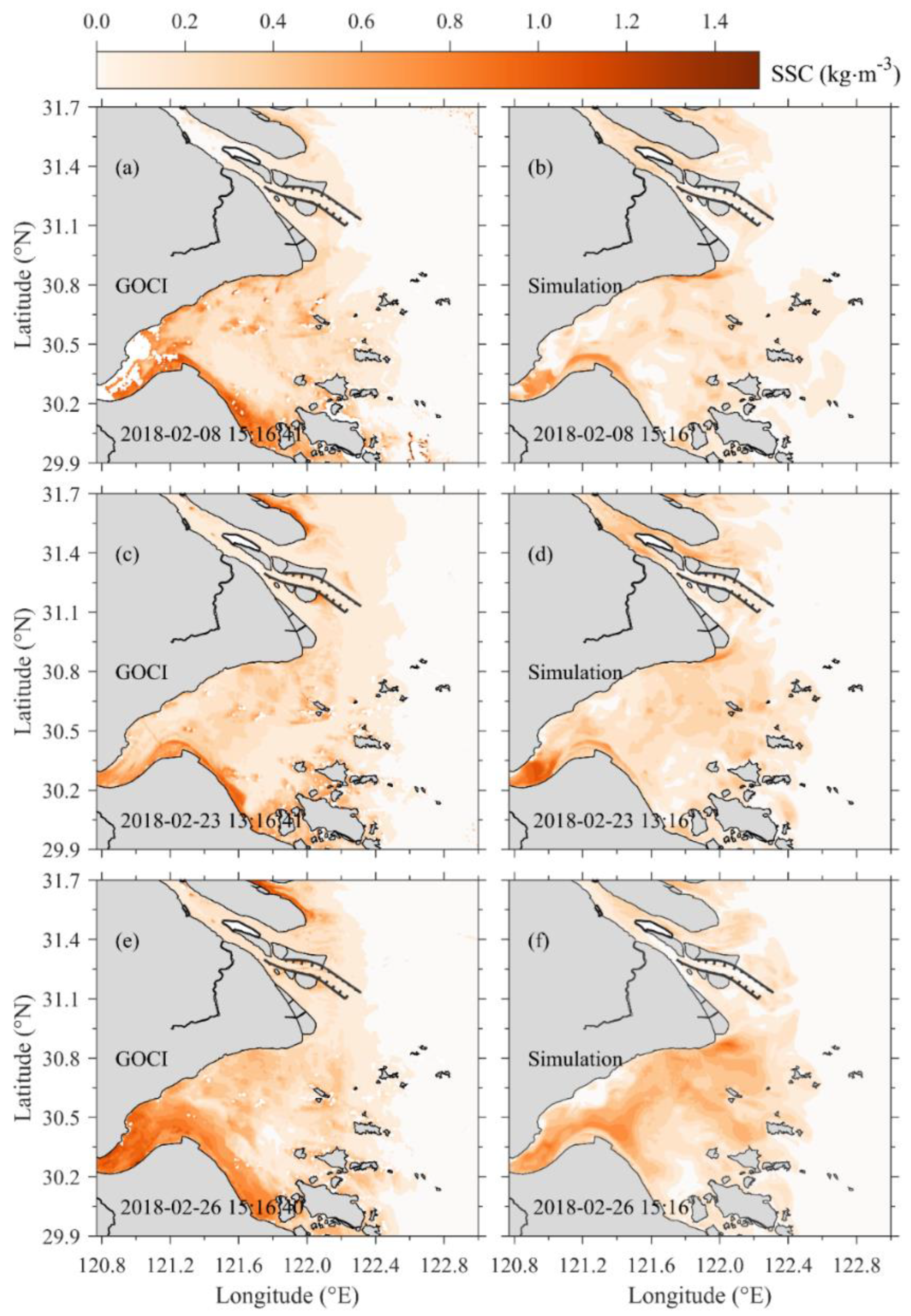
  29. Hu, Y.K.; Yu, Z.F.; Zhou, B.; Li, Y.; Yin, S.J.; He, X.Q.; Peng, X.X.; Shum, C.K. Tidal-driven variation of suspended sediment in Hangzhou Bay based on GOCI data. Int. J. Appl. Earth Obs. Geoinf. 2019, 82, 101920. [Google Scholar] [CrossRef]
  30. Yang, X.F.; Mao, Z.H.; Huang, H.Q.; Zhu, Q.K. Using GOCI retrieval data to initialize and validate a sediment transport model for monitoring diurnal variation of SSC in Hangzhou Bay, China. Water 2016, 8, 108. [Google Scholar] [CrossRef]
  31. Wang, D.S.; Cao, A.Z.; Zhang, J.C.; Fan, D.D.; Liu, Y.Z.; Zhang, Y. A three-dimensional cohesive sediment transport model with data assimilation: Model development, sensitivity analysis and parameter estimation. Estuar. Coast. Shelf Sci. 2018, 206, 87–100. [Google Scholar] [CrossRef]
  32. Zhang, J.C.; Chu, D.D.; Wang, D.S.; Cao, A.Z.; Lv, X.Q.; Fan, D.d. Estimation of spatially varying parameters in three-dimensional cohesive sediment transport models by assimilating remote sensing data. J. Mar. Sci. Technol. 2018, 23, 319–332. [Google Scholar] [CrossRef]
  33. Blumberg, A.F. A Primer for ECOM-si; Technical Report; HydroQual, Inc.: Mahwah, NJ, USA, 1994; p. 66. [Google Scholar]
  34. Blumberg, A.F.; Mellor, G.L. A description of a three-dimensional coastal ocean circulation model. Three-Dimens. Coast. Ocean Models 1987, 4, 1–16. [Google Scholar]
  35. Arakawa, A.; Lamb, V.R. Computational design of the basic dynamical processes of the UCLA general circulation model. Gen. Circ. Models Atmos. 1977, 17, 173–265. [Google Scholar]
  36. Chen, C.S.; Zhu, J.R.; Zheng, L.Y.; Ralph, E.; Budd, J.W. A non-orthogonal primitive equation coastal ocean circulation model: Application to Lake Superior. J. Gt. Lakes Res. 2004, 30, 41–54. [Google Scholar] [CrossRef]
  37. Mellor, G.L.; Yamada, T.J. Development of a turbulence closure model for geophysical fluid problems. Rev. Geophys. 1982, 20, 851–875. [Google Scholar] [CrossRef]
  38. Smagorinsky, J. General circulation experiments with the primitive equations: I. The basic experiment. Mon. Weather Rev. 1963, 91, 99–164. [Google Scholar] [CrossRef]
  39. Wu, H.; Zhu, J.R. Advection scheme with 3rd high-order spatial interpolation at the middle temporal level and its application to saltwater intrusion in the Changjiang Estuary. Ocean Model. 2010, 33, 33–51. [Google Scholar] [CrossRef]
  40. Casulli, V.; Cattani, E. Stability, accuracy and efficiency of a semi-implicit method for three-dimensional shallow water flow. Comput. Math. Appl. 1994, 27, 99–112. [Google Scholar] [CrossRef] [Green Version]
  41. Wu, H.; Zhu, J.R.; Shen, J.; Wang, H. Tidal modulation on the Changjiang River plume in summer. J. Geophys. Res. Ocean. 2011, 116. [Google Scholar] [CrossRef]
  42. Mellor, G.L.; Yamada, T.J. A hierarchy of turbulence closure models for planetary boundary layers. J. Atmos. Sci. 1974, 31, 1791–1806. [Google Scholar] [CrossRef]
  43. Song, D.H.; Wang, X.H. Suspended sediment transport in the Deepwater Navigation Channel, Yangtze River Estuary, China, in the dry season 2009: 2. Numerical simulations. J. Geophys. Res. Ocean. 2013, 118, 5568–5590. [Google Scholar] [CrossRef]
  44. Luo, Z.F.; Zhu, J.R.; Wu, H.; Li, X.Y. Dynamics of the sediment plume over the Yangtze Bank in the Yellow and East China Seas. J. Geophys. Res. Ocean. 2017, 122, 10073–10090. [Google Scholar] [CrossRef]
  45. Van Prooijen, B.C.; Winterwerp, J.C. A stochastic formulation for erosion of cohesive sediments. J. Geophys. Res. Ocean. 2010, 115. [Google Scholar] [CrossRef]
  46. Ge, J.Z.; Shen, F.; Guo, W.Y.; Chen, C.S.; Ding, P.X. Estimation of critical shear stress for erosion in the C hangjiang E stuary: A synergy research of observation, GOCI sensing and modeling. J. Geophys. Res. Ocean. 2015, 120, 8439–8465. [Google Scholar] [CrossRef]
  47. Lumborg, U. Modelling the deposition, erosion, and flux of cohesive sediment through Øresund. J. Mar. Syst. 2005, 56, 179–193. [Google Scholar] [CrossRef]
  48. Pandoe, W.W.; Edge, B.L. Case study for a cohesive sediment transport model for Matagorda Bay, Texas, with coupled ADCIRC 2D-transport and SWAN wave models. J. Hydraul. Eng. 2008, 134, 303–314. [Google Scholar] [CrossRef]
  49. Van Rijn, L.C. Principles of Sediment Transport in Rivers, Estuaries and Coastal Seas; Aqua Publications: Amsterdam, The Netherlands, 1993; Volume 1006. [Google Scholar]
  50. Shi, B.W.; Yang, S.L.; Wang, Y.P.; Bouma, T.J.; Zhu, Q. Relating accretion and erosion at an exposed tidal wetland to the bottom shear stress of combined current–wave action. Geomorphology 2012, 138, 380–389. [Google Scholar] [CrossRef]
  51. Mehta, A.J.; Lee, S.C. Problems in linking the threshold condition for the transport of cohesionless and cohesive sediment grain. J. Coast. Res. 1994, 10, 170–177. [Google Scholar]
  52. Taki, K. Critical shear stress for cohesive sediment transport. In Proceedings in Marine Science; Elsevier: Amsterdam, The Netherlands, 2000; Volume 3, pp. 53–61. [Google Scholar]
  53. Yang, M.Q.; Wang, G.L. The incipient motion formulas for cohesive fine sediments. J. Basic Sci. Eng. 1995, 3, 99–109, (In Chinese with English Abstract). [Google Scholar]
  54. Van Rijn, L.C. Unified view of sediment transport by currents and waves. I: Initiation of motion, bed roughness, and bed-load transport. J. Hydraul. Eng. 2007, 133, 649–667. [Google Scholar] [CrossRef] [Green Version]
  55. Fofonoff, N.P.; Millard, R.C., Jr. Algorithms for the Computation of Fundamental Properties of Seawater. Unesco Tech. Pap. Mar. Sci. 1983, 44, 53. [Google Scholar]
  56. Winterwerp, J.C. Stratification effects by cohesive and noncohesive sediment. J. Geophys. Res. Ocean. 2001, 106, 22559–22574. [Google Scholar] [CrossRef]
  57. Allen, G.P.; Salomon, J.C.; Bassoullet, P.; Du Penhoat, Y.; De Grandpre, C. Effects of tides on mixing and suspended sediment transport in macrotidal estuaries. Sediment. Geol. 1980, 26, 69–90. [Google Scholar] [CrossRef]
  58. Wang, X.H.; Byun, D.S.; Wang, X.L.; Cho, Y.K. Modelling tidal currents in a sediment stratified idealized estuary. Cont. Shelf Res. 2005, 25, 655–665. [Google Scholar] [CrossRef]
  59. Ge, J.Z.; Chen, C.S.; Wang, Z.B.; Ke, K.T.; Yi, J.X.; Ding, P.X. Dynamic response of the fluid mud to a tropical storm. J. Geophys. Res. Ocean. 2020, 125, e2019JC015419. [Google Scholar] [CrossRef]
  60. Ge, J.Z.; Zhou, Z.Y.; Yang, W.L.; Ding, P.X.; Chen, C.S.; Wang, Z.B.; Gu, J.H. Formation of concentrated benthic suspension in a time-dependent salt wedge estuary. J. Geophys. Res. Ocean. 2018, 123, 8581–8607. [Google Scholar] [CrossRef]
  61. Trowbridge, J.H.; Kineke, G.C. Structure and dynamics of fluid muds on the Amazon continental shelf. J. Geophys. Res. Ocean. 1994, 99, 865–874. [Google Scholar] [CrossRef]
  62. Wolanski, E.; Chappell, J.; Ridd, P.; Vertessy, R. Fluidization of mud in estuaries. J. Geophys. Res. Ocean. 1988, 93, 2351–2361. [Google Scholar] [CrossRef]
  63. Wang, X.H. Tide-induced sediment resuspension and the bottom boundary layer in an idealized estuary with a muddy bed. J. Geophys. Res. Ocean. 2002, 32, 3113–3131. [Google Scholar] [CrossRef]
  64. Hwang, K.N. Erodibility of Fine Sediment in Wave-Dominated Environments. Master’s Thesis, University of Florida, Gainesville, FL, USA, 1989. [Google Scholar]
  65. Mehta, A.J.; McAnally, W.H. Fine grained sediment transport. In Sedimentation Engineering: Processes, Measurements, Modeling, and Practice; American Society of Civil Engineers: Reston, VA, USA, 2008; pp. 253–306. [Google Scholar]
  66. Huang, S.; Han, N.; Zhong, X. Analysis of siltation at mouth bar of the Yangtze River Estuary. In Proceedings of the International Symposium on River Sedimentation, Beijing, China, 24–29 March 1980. [Google Scholar]
  67. Wang, X.H.; Pinardi, N. Modeling the dynamics of sediment transport and resuspension in the northern Adriatic Sea. J. Geophys. Res. Ocean. 2002, 107, 18-11–18-23. [Google Scholar] [CrossRef]
  68. Sternberg, R.W.; Berhane, I.; Ogston, A.S.J.M.G. Measurement of size and settling velocity of suspended aggregates on the northern California continental shelf. Mar. Geol. 1999, 154, 43–53. [Google Scholar] [CrossRef]
  69. Shi, Z.; Zhou, H.J. Controls on effective settling velocities of mud flocs in the Changjiang Estuary, China. Hydrol. Process. 2004, 18, 2877–2892. [Google Scholar] [CrossRef]
  70. Wan, Y.; Wu, H.; Roelvink, D.; Gu, F. Experimental study on fall velocity of fine sediment in the Yangtze Estuary, China. Ocean Eng. 2015, 103, 180–187. [Google Scholar] [CrossRef]
  71. Yang, Y.; Wang, Y.P.; Li, C.; Gao, S.; Shi, B.; Zhou, L.; Wang, D.; Li, G.; Dai, C. On the variability of near-bed floc size due to complex interactions between turbulence, SSC, settling velocity, effective density and the fractal dimension of flocs. Geo-Mar. Lett. 2016, 36, 135–149. [Google Scholar] [CrossRef]
  72. McAnally, W.H.; Teeter, A.; Schoellhamer, D.; Friedrichs, C.; Hamilton, D.; Hayter, E.; Shrestha, P.; Rodriguez, H.; Sheremet, A.; Kirby, R. Management of fluid mud in estuaries, bays, and lakes. II: Measurement, modeling, and management. J. Hydraul. Eng. 2007, 133, 23–38. [Google Scholar] [CrossRef]
  73. Costa, R.G.; Mehta, A.J. Flow-fine sediment hysteresis in sediment-stratified coastal waters. In Coastal Engineering; American Society of Civil Engineers: Reston, VA, USA, 1991; pp. 2047–2060. [Google Scholar]
  74. Wiberg, P.L.; Sherwood, C.R. Calculating wave-generated bottom orbital velocities from surface-wave parameters. Comput. Geosci. 2008, 34, 1243–1262. [Google Scholar] [CrossRef]
  75. Mellor, G.; Blumberg, A. Wave breaking and ocean surface layer thermal response. J. Phys. Oceanogr. 2004, 34, 693–698. [Google Scholar] [CrossRef]
  76. Booij, N.; Ris, R.C.; Holthuijsen, L.H. A third-generation wave model for coastal regions: 1. Model description and validation. J. Geophys. Res. Ocean. 1999, 104, 7649–7666. [Google Scholar] [CrossRef]
  77. Lyu, H.H.; Zhu, J.R. Impact of the bottom drag coefficient on saltwater intrusion in the extremely shallow estuary. J. Hydrol. 2018, 557, 838–850. [Google Scholar] [CrossRef]
  78. Qiu, C.; Zhu, J.R. Influence of seasonal runoff regulation by the Three Gorges Reservoir on saltwater intrusion in the Changjiang River Estuary. Cont. Shelf Res. 2013, 71, 16–26. [Google Scholar] [CrossRef]
  79. Murphy, A.H. Skill scores based on the mean square error and their relationships to the correlation coefficient. Mon. Weather Rev. 1988, 116, 2417–2424. [Google Scholar] [CrossRef]
  80. Warner, J.C.; Geyer, W.R.; Lerczak, J.A. Numerical modeling of an estuary: A comprehensive skill assessment. J. Geophys. Res. Ocean. 2005, 110. [Google Scholar] [CrossRef]
  81. Willmott, C.J. On the validation of models. Phys. Geogr. 1981, 2, 184–194. [Google Scholar] [CrossRef]
  82. Shen, F.; Zhou, Y.X.; Li, J.F.; He, Q.; Verhoef, W. Remotely sensed variability of the suspended sediment concentration and its response to decreased river discharge in the Yangtze estuary and adjacent coast. Cont. Shelf Res. 2013, 69, 52–61. [Google Scholar] [CrossRef]
  83. Shen, F.; Zhou, Y.X.; Peng, X.Y.; Chen, Y.L. Satellite multi-sensor mapping of suspended particulate matter in turbid estuarine and coastal ocean, China. Int. J. Remote Sens. 2014, 35, 4173–4192. [Google Scholar] [CrossRef]
  84. Bian, C.W.; Jiang, W.S.; Quan, Q.; Wang, T.; Greatbatch, R.J.; Li, W. Distributions of suspended sediment concentration in the Yellow Sea and the East China Sea based on field surveys during the four seasons of 2011. J. Mar. Syst. 2013, 121, 24–35. [Google Scholar] [CrossRef]
Figure 1. Map of Hangzhou Bay and Changjiang Estuary. Black triangle: the anchored ship stations; thick black line: section from Nanhui Cape to Qiqu Archipelago.
Jmse 10 01248 g001
Figure 2. Numerical model domain and grid (a), and an enlarged view of the model grid in Hangzhou Bay (b).
Jmse 10 01248 g002
Figure 3. Distribution of median sediment diameter (a) and water content (b) of seabed sediment in Hangzhou Bay and the Changjiang Estuary.
Jmse 10 01248 g003
Figure 4. Comparisons between the observed data (red dots) and simulated results (black line) at measured site A. The left column represents neap tide, and the right column represents spring tide. (a,b) Surface velocity; (c,d) bottom velocity; (e,f) surface direction; (g,h) bottom direction; (i,j) surface salinity; (k,l) bottom salinity; (m,n) surface SSC; and (o,p) bottom SSC (loss of surface SSC during spring tide due to the typhoon).
Jmse 10 01248 g004
Figure 5. Comparisons between the observed data (red dots) and simulated results (black line) at measured site B. The left column represents neap tide, and the right column represents spring tide. (a,b) Surface velocity; (c,d) bottom velocity; (e,f) surface direction; (g,h) bottom direction; (i,j) surface salinity; (k,l) bottom salinity; (m,n) surface SSC; and (o,p) bottom SSC (loss of surface SSC during spring tide due to the typhoon).
Jmse 10 01248 g005
Figure 6. Comparison of the satellite inversion of SSC with simulated surface SSC fields at 15:16, 08 February 2018, 13:16, 23 February 2018 and 15:16, 26 February 2018. Surface SSC derived from GOCI satellite data (a,c,e); surface SSC simulated by the model (b,d,f).
Jmse 10 01248 g006
Figure 7. Distribution of residual water level during neap tide (left panel) and spring tide (right panel) in summer (a,b) and winter (c,d).
Jmse 10 01248 g007
Figure 8. Distribution of the RUWF and salinity in the surface layer (upper panel) and bottom layer (lower panel) during neap tide (a,c) and spring tide (b,d) in summer (contours represent salinity and the arrows represent RUWF).
Jmse 10 01248 g008
Figure 9. Distribution of the RUWF and salinity in the surface layer (upper panel) and bottom layer (lower panel) during neap tide (a,c) and spring tide (b,d) in winter.
Jmse 10 01248 g009
Figure 10. Distribution of the RUWF in the whole layer during neap tide (left panel) and spring tide (right panel) in summer (a,b) and winter (c,d).
Jmse 10 01248 g010
Figure 11. Distribution of the RUSF and SSC in the surface layer (upper panel) and bottom layer (lower panel) during neap tide (a,c) and spring tide (b,d) in summer (color images represent SSC and arrows represent RUSF).
Jmse 10 01248 g011
Figure 12. Distribution of the RUSF and SSC in the surface layer (upper panel) and bottom layer (lower panel) during neap tide (a,c) and spring tide (b,d) in winter.
Jmse 10 01248 g012
Figure 13. Distribution of the RUSF in the whole layer during neap tide (left panel) and spring tide (right panel) in summer (a,b) and winter (c,d); thick black line: section from Nanhui Cape to Qiqu Archipelago.
Jmse 10 01248 g013
Figure 14. Vertical profile distributions of salinity (a,b) and SSC (c,d) along the section from Nanhui Cape to Qiqu Archipelago during neap tide (left panel) and spring tide (right panel) in summer.
Jmse 10 01248 g014
Figure 15. Temporal variation in surface SSC (a,b), bottom SSC (c,d), vertically averaged eddy diffusivity (Kv) (e,f) and bottom drag coefficient (Cd) (g,h) at measured sites A (left panel) and B (right panel). Black line: with SSC stratification; green line: without SSC stratification; red dots: observed SSC.
Jmse 10 01248 g015
Figure 16. The SSC difference between Exp 1 and the control experiment in the surface layer (upper panel), bottom layer (middle panel), and whole layer (lower panel) during neap tide (a,c,e) and spring tide (b,d,f).
Jmse 10 01248 g016
Figure 17. Distribution of tidally averaged barotropic pressure gradient force (a), vertically averaged baroclinic pressure gradient force (b), resultant force of wind stress and bottom friction (c), and the RUSF in the whole layer without baroclinic pressure gradient force (d) during neap tide in summer.
Jmse 10 01248 g017
Figure 18. Distribution of tidally averaged barotropic pressure gradient force (a), vertically averaged baroclinic pressure gradient force (b), resultant force of wind stress and bottom friction (c), and the RUSF in the whole layer without baroclinic pressure gradient force (d) during spring tide in summer.
Jmse 10 01248 g018
Table 1. Parameters in the sediment model.
ParameterValueReference
M (kg·m−2·s−1)3.0 × 10⁻⁵Tested
α 0.67Tested
β 0.30[52]
p c s 0.25[54]
υ (m2·s−1)1.36 × 10⁻⁶[49]
ρs (kg·m−3)1250[72]
C0 (kg·m−3)0.20[65]
m10.10[73]
m26.20[73]
n11.20[73]
n21.60[73]
Table 2. Correlation coefficients (CC), root-mean-square error (RMSE), and skill scores (SS) for comparison of modeled and observed water velocity, salinity, and suspended sediment at the measuring stations.
Skill AssessmentSite ASite B
CCRMSESSCCRMSESS
Surface velocity in the neap tide0.940.15 m/s0.970.940.15 m/s0.97
Bottom velocity in the neap tide0.870.09 m/s0.920.940.07 m/s0.97
Surface velocity in the spring tide0.930.22 m/s0.960.960.15 m/s0.98
Bottom velocity in the spring tide0.900.15 m/s0.950.900.15 m/s0.94
Surface salinity in the neap tide0.740.900.840.860.810.85
Bottom salinity in the neap tide0.970.610.950.930.620.89
Bottom salinity in the spring tide0.731.390.800.550.810.74
Surface SSC in the neap tide0.640.12 kg·m−30.780.780.11 kg·m−30.87
Bottom SSC in the neap tide0.470.31 kg·m−30.600.670.63 kg·m−30.64
Bottom SSC in the spring tide0.631.19 kg·m−30.780.560.93 kg·m−30.75
Table 3. NTWF and NTSF across the section from Nanhui Cape to the Qiqu Archipelago. Negative values indicate flow into Hangzhou Bay, and positive values indicate flow into the Changjiang Estuary.
PhasesNTWF (109 m3)NTSF (109 kg)
Spring tide in summer−2.91−4.16
Neap tide in summer4.292.44
One month in summer−7.81−4.80
Spring tide in winter−2.27−4.30
Neap tide in winter−0.160.93
One month in winter−13.4−21.6
Publisher’s Note: MDPI stays neutral with regard to jurisdictional claims in published maps and institutional affiliations.

