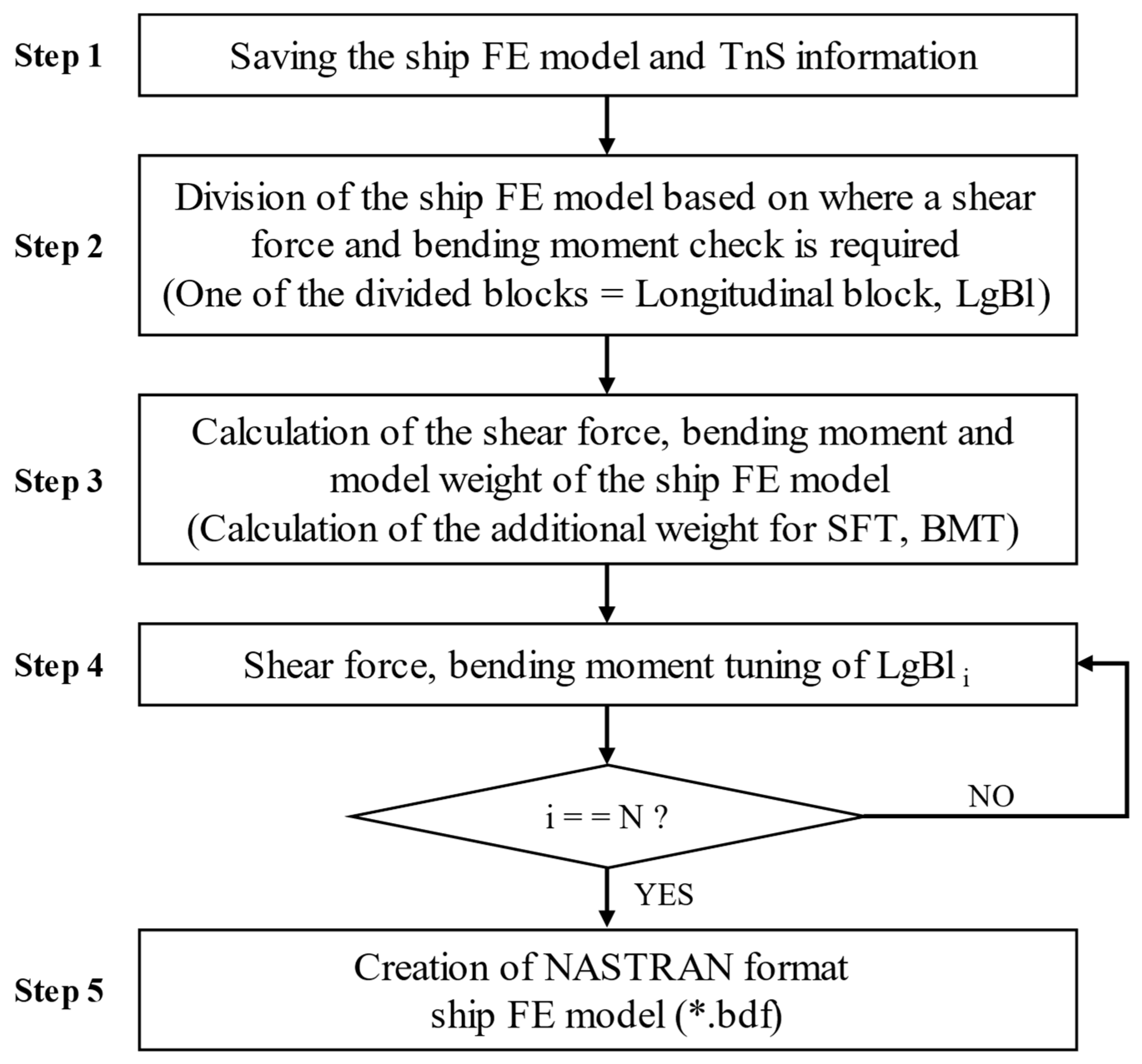
In Steps 3, 4, and 5 of
Figure 1, the detailed process of SFT and BMT for the ship FE model that has completed the WD is as follows. Instead of performing SFT and BMT simultaneously, BMT was performed only when required after SFT. This is because a ship FE model that has completed the WD and SFT often satisfies the target values of the weight, COG, and SF at each DP, and thus has also satisfied the value of the BM under these conditions. However, BMT is required when the BM deviates from the target tolerance because of a slight difference in structural geometry between the model and ship, precision of the model data, or accuracy of the SFT values.
Figure 4 shows the detailed process of SFT and BMT. If the target values of the SF and BM are obtained after SFT, tuning is completed. Otherwise, BMT is performed, and tuning is completed if the target value is obtained after BMT. In the ship FE model coordinate system, “Xcog,” “Ycog,” and “Zcog” are the X—(longitudinal), Y—(transverse), and Z—(height) components of the COG location.
2.2.1. Detailed Process of SFT
First, only SFT was performed for the ship FE model. Before the SF and BM were tuned for the ship FE model that completed the WD, they were significantly different from the target values. Thus, the SFT values at each DP of the ship FE model were calculated using the SF values of the ship FE model with WD analysis results, the longitudinal SF curve values of the TnS data, and the grid weight information. This is required to tune the SF of the current ship FE model to that of the actual ship. Based on the calculated value,
was added or subtracted from each LgBl of the ship FE model for SFT.
Figure 5 and Equations (2)–(2.e) show the SFT value and the
calculation method when the number of DPs is three for the ship FE model, and the SF is calculated in the direction from the stern to the bow. Regarding
LgBl1 and the DP of
, the SF increases by
, and as a result, it changes from
to the target value
(Equation (2)). Further, the weight of
LgBl1 changes from
to
(Equation (2.a)). Moreover, when the SFs of
LgBl2 and
and that of
LgBl3 and
are adjusted in a similar manner, the SF of the ship FE model coincides with the TnS SF, which is the target value, and the total weight becomes equal to the target value, that is, the weight after WD Equations (2.b)–(2.e).
Prior to SFT, the ship FE model satisfies the target weight and COG because the WD has been completed. However, during SFT, the ship FE model COG is affected by the change in the COG of each LgBl. Therefore, when the SF is tuned by distributing the previously calculated
to each LgBl, the target COG that must be satisfied by each LgBl is calculated to tune the ship FE model COG to the target COG. When the target SF, weight, and Xcog are satisfied through SFT for all LgBls, those values associated with the completed SFT of the ship FE model will also satisfy the target values. Subsequently, the Ycog and Zcog of each LgBl were also tuned to the Ycog and Zcog of the ship FE model. The calculating method for the target Xcog of all LgBls when the ship FE model is separated into three LgBl parts is detailed in
Figure 5 and Equations (3)–(3.c). The direction of the positive x-axis is the bow direction in
Figure 5. Equation (3.c) shows the calculation method of
A, which means the coefficient of Xcog moving the length of the LgBl. Further, regarding
LgBl1, the Xcog prior to SFT was
with a weight of
and a length of
. After SFT, the Xcog moved by
from
to
and the weight was
. Thus, when the Xcog of all LgBls is changed by
in the same method, the Xcog of the ship FE model,
, coincides with the target value of
. Moreover, the total weight of the ship FE model,
, is maintained and coincides with the target value of
. In addition, as the Ycog and Zcog of each LgBl are identical to the target values, the transverse (Ycog) and height (Zcog) components of the ship FE model COG location also coincide with the target values.
where
Figure 6 and
Figure 7 show the detailed process of weight addition to each
for SFT, and the description is as follows.
Figure 7a–c show one
, where the current Xcog of the LgBl is
, and the target Xcog is
. The LgBl was divided into two based on
, as shown in
Figure 7a, and the right side of the LgBl is referred to as partial block 1 (
PB1), while the left side is partial block 2 (
PB2). The weight and Xcog of
PB1 are
and
, and those of
PB2 are
and
, respectively. The weight added to
for SFT was
calculated using Equations (2)–(3.c). At this time, the weights added to
PB1 and
PB2 are
and
, respectively. As shown in
Figure 7, for
to coincide with
,
must be moved to the right by
. Furthermore,
and
were calculated using Equation (4), and only
was added to
of
PB2. In this case,
was not added to
PB1 because its value is zero. By contrast, if
is on the left side of
, only
is added to
of
PB1 because
must be moved to the left by
. Similarly,
is not added to
PB2 because its value is zero. To satisfy the Xcog, Ycog, and Zcog target values, only 10% of
and
were added to the partial block. Further, 10% weight was added to each grid included in the partial block, as calculated using Equations (5)–(5.a). The weight added to the grid was calculated based on the ratio of the current grid weight to the current LgBl weight. Thus, the above process is a method to achieve the Xcog target value during SFT. The SFT, Ycog, and Zcog adjustments are similar to that of the above Xcog method and are shown in
Figure 7b,c, respectively. As evident, when adjusting the Ycog, the LgBl is divided into left and right partial blocks based on the current Ycog (
Figure 7b), whereas, when adjusting the Zcog, the LgBl is divided into top and bottom blocks based on the current Zcog (
Figure 7c). Furthermore, when SFT and adjustments are conducted in the order Xcog → Zcog → Ycog (1 iteration), and if COG
does not meet the target value
, the process is repeated.
where
where
In Equations (5)–(5.a),
is the weight added to
for the SFT and adjustment of Xcog in the
iteration, and
and
are the weights added for the SFT and adjustment of Ycog and Zcog, respectively.
Figure 8 shows the weight added to
in the
iteration, prior to the addition of the weight; the grid weight is
whereas it is
after weight addition.
The weight added to
in the
iteration in Equations (5)–(5.a) and (6)–(6.a) is
, which is equal to the sum of the weight added
to
in the
iteration. Further, the total weight added to the grid during the entire iteration is the same as the weight added
to
during the entire iteration. When completing the iteration, the COG satisfies the target value; however, the SF does not satisfy the target value. Therefore, the weight
is added to
using Equations (6)–(6.b) such that the total weight added to the
becomes
and consequently, the SF is tuned to the target value. At this moment, to keep the COG of the LgBl to the target value, the weight
is distributed and assigned to the grid included in the LgBl using Equations (6)–(6.b), and the added weight to the grid is
.
where
If the SF and COG of all LgBls are adjusted in this way, the total weight, SF, and COG of the ship FE model can meet the target values. Upon completion of SFT, the SFT results and the BM value are examined through global ship analysis. If the total weight, COG, and SF curve of the ship FE model satisfy the target values, the BM value will also satisfy the target value. However, there exist cases where the BM cannot satisfy the target tolerance. In such cases, BMT is performed.
2.2.2. Detailed Process of the BMT
The detailed process of BMT for the ship FE model that has completed SFT is as follows. Because the ship FE model that has completed SFT satisfies the target values for the weight, COG, and SF, the COG of each LgBl must be adjusted for BMT while maintaining the current status of these values. Thus, the BMT value at each DP of the ship FE model is calculated using the BM values obtained from the global ship model analysis, longitudinal BM curve of the ship obtained from the TnS data, and grid weight information. This is required to tune the current BM of the ship FE model to the TnS ship BM. To perform BMT using the calculated values, the movement distance required for the COG of each LgBl is calculated.
Figure 9 and Equations (7)–(7.g) show the method of calculating the BMT value and COG when the ship FE model is separated into three sections. The BM is calculated in the direction from the stern to the bow, as in SFT. In contrast to SFT, wherein
is added or subtracted, the COG is moved by adjusting the position and ratio of
distributed in each LgBl without the addition of
for BMT. Moreover, regarding
LgBl1 and the DP of
, when Xcog changes from
to
during BMT, the BM changes by
and meets the target value of
at
, while the weight of
LgBl1 is maintained at
. Here, as the Ycog and Zcog of each LgBl were tuned to the target Ycog and Zcog values, the transverse (Ycog) and height (Zcog) components of the ship FE model COG location also coincided with the target values. Further, if the BM of
LgBl2 and
and that of
LgBl3 and
are tuned in the same method, the BM of the ship FE model coincides with the target TnS BM. Moreover, the weight and COG are maintained at the target values.
where
The detailed method for adjusting the COG of each LgBl for BMT is the same as that of the SFT method explained in
Figure 6. Similar to 10% of
or
being added to
PB1 or
PB2 for SFT, 10% of the current LgBl weight
was added to
PB1 or
PB2 for BMT. The weight added to the grid included in each PB is calculated using Equations (8) and (8.a), and that added to
in the
iteration is
. This process is repeated until the COG
of the LgBl satisfies the target value
. Upon completion of the iterations, although the COG satisfies the target value, the BM cannot satisfy the target value.
where
Therefore, the excess weight
is removed from the LgBl such that the weight of the LgBl is equal to the weight prior to BMT (weight after SFT). At this moment, excess weight
is removed from the grid in the LgBl using Equations (9)–(9.b) to maintain the COG of the LgBl at the target value.
where
Equations (10) and (10.a) represent the final
that is added to
and
in
following the application of SFT and BMT. If the SF, BM, and COG satisfy the target values by SFT, the weight
that is added to the grid based on the BMT in Equation (10.a) becomes zero.
where
Thus, by adjusting the BM and COG of all LgBls, the total weight, COG, SF, and BM of the ship FE model can coincide with the required target values.


 ,
, 


