Article

Characterization and Modeling of Doppler Spectra for Offshore UHF-Band Sea Clutter at Low Grazing Angles

1
School of Physics, Xidian University, Xi’an 717071, China
2
National Key Laboratory of Electromagnetic Environment, China Research Institute of Radiowave Propagation, Qingdao 266107, China
*
Author to whom correspondence should be addressed.
J. Mar. Sci. Eng. 2023, 11(10), 1901; https://doi.org/10.3390/jmse11101901
Submission received: 11 August 2023 / Revised: 21 September 2023 / Accepted: 28 September 2023 / Published: 30 September 2023
(This article belongs to the Section Physical Oceanography)

Abstract

:
The Doppler spectra of sea echoes, which contain abundant information on floating scatterers, are important for exploring the characteristics of sea clutter. Using sea clutter data at low grazing angles observed by a coherent ultra-high frequency (UHF) radar located on Lingshan Island in the Yellow Sea, China, this study conducted detailed research on the characteristics of Doppler spectra with multiple ocean parameters, including grazing angle, significant wave height (SWH), and wave directions. The effect of sea echoes with different local normalized intensities on short-time Doppler spectra was further studied. The results indicate that with increasing sea states, the bimodal behavior of Doppler spectra, an evident phenomenon of Bragg scattering, gradually weakens. The frequency shifts of the mean spectra increased linearly with increasing SWH and wind speed, decreased linearly with increasing grazing angle, and decreased with the cosine value of the relative wave direction angles. In comparison, frequency shifts of the short-time spectra increased with increasing sea states and local echo intensities but fluctuated around a fixed value after reaching a certain extent. For spectral widths, the grazing angle is a significant influencing factor, with its broadening trend evident with a decrease in the grazing angle, whereas other ocean parameters, such as wave direction and wind direction, have no apparent influence. Considering the major contributions of the parameters, semi-empirical models for the mean spectral frequency shifts, mean spectral widths and short-time spectral frequency shifts were proposed. By verifying the measured data and predicted results, the models exhibited good prediction accuracy and applicability. The proposed inferences and models are helpful for understanding low grazing angle UHF-band sea clutter characteristics and improving target detection algorithms in offshore areas. These findings supplement previous studies on sea clutter Doppler spectra.

1. Introduction

Sea clutter is a major source of interference in the radar detection of targets on the ocean surface [1]. Employing Doppler processing of coherent radar sea returns is an effective method for distinguishing targets from clutter [2]. However, some targets with radial velocity and low radar cross section will have Doppler shifts that are not significantly different from the Doppler spectra of the clutter. Thus, radar designers must have a detailed understanding of the characteristics of Doppler spectra for all conditions that are likely to be encountered [3,4].
Doppler characteristics from sea echoes have been the subject of extensive scientific investigations over the past decades, and significant progress has already been made in understanding the physical and statistical properties of Doppler spectra. Crombie [5] first discovered the Bragg scattering phenomenon from sea clutter in the high frequency (HF)-band. From this discovery, the first-order and second-order Doppler models based on a small perturbation method were established by [6,7,8]. Chen et al. [9] analyzed the simulated echo Doppler spectra for various parameters based on a shore-to-air bistatic HF radar model. Subsequently, more investigations focused on microwave bands. By analyzing L-, X-, and Ku-band sea clutter, Plant and Keller [10] found evidence of Bragg scattering in microwave Doppler spectra. Moreover, they hypothesized that Bragg scattering was the main source of microwave sea returns at moderate incidence angles and low-to-moderate wind speeds.
As the research progressed, some special characteristics of Doppler spectra, different from Bragg scattering, were observed. By analyzing wave tank microwave data, Lee [11,12] found a non-Bragg-scattering phenomenon and created a new Doppler model containing three components, Gaussian, Lorentzian, and Voigtian, the last two components of which correspond to non-Bragg-scattering mechanism. Walker [13,14] developed a more simplified Doppler model by analyzing wave tank and radar sea clutter data from a cliff. The model provided a possible physical understanding of electromagnetic wave scattering by assuming that the entire Doppler spectrum is the sum of Gaussian line shapes denoted by three scattering mechanisms–Bragg, whitecap, and burst.
Moreover, Greco [15] described an autoregressive nonstationary process to model physical phenomena. Ward [3,16] proposed a temporally varying short-time Doppler spectra model. Based on these studies, Zhang et al. [17] proposed a time-varying Doppler spectra model with an additional velocity frequency shift that simulated short-time spectra well with longer observation times and mean spectra under complex conditions. Watts [18] proposed a more general approach to clutter simulation by representing the time and distance evolution of the Doppler spectra. In recent years, using sufficient work by Watts [19,20] and Rosenberg [21,22,23] on the sea clutter data of Ingara radar at middle and high grazing angles, the “evolving Doppler model” was proposed and gradually extended from a single Gaussian form to the bimodal form. Based on these models, Rosenberg [24] provided a parameterized model that captured the observed behavior over all possible integration times. Yurovsky et al. [25] proposed an empirical modulation transfer function parameterization for Ka-band sea clutter Doppler spectra based on polynomial fitting as a function of observation geometry and wind. The above studies and models have well characterized the sea clutter spectral characteristics in microwaves and millimeter waves; however, studies on the spectral characteristics in the ultra HF (UHF)-band have been limited, and the consistency of its sea clutter spectral characteristics with those of microwaves has not been clear.
In recent years, some measurements of sea clutter in coastal environments were also carried out by researchers. Norland et al. [26] made a comparison of measured sea clutter and wave rider buoy data in open sea and coastal waters and found that sea clutter in coastal regions is spikier than that of open sea when the range resolution is becoming smaller, which seriously affected small target detection. Del-Rey-Maestre et al. [27] made a statistical analysis of bistatic sea radar clutter data acquired using a UHF radar located on the Spanish North-west coast, and they found that the zero Doppler shift and values close to it present high variability, which should be characterized by a non-homogeneous clutter. Fabbro et al. [28] held a coastal measurement campaign in the Mediterranean Sea region, and the mean Doppler spectra velocity is presented and analyzed according to grazing and azimuth angles at the C- and Ka-band. Navarro et al. [29] proposed a novel method based on filtering and interpolation approaches to estimate the sea state parameters in shallow waters using X-band navigation radar. Reviewing the existing offshore sea clutter measurement research shows the characteristics of discrete and unsystematic, especially for the UHF-band sea clutter spectra; either the parameters are not comprehensive, or the frequency band is not covered. This article happens to be a good supplement.
The UHF-band radar has a longer detection range and better anti-stealth than the microwave-band radar, as well as better directionality than the HF/very HF-band radar. Thus, it has many applications for early warning, anti-stealth, and target detection. The characteristics of UHF-band sea clutter, especially at low grazing angles and high sea states, have received increasing attention. Most of the existing spectral models use the Gaussian function to fit the line shapes of Doppler spectra, and frequency shift and spectral width are particularly important parameters. Using the analysis of Ingara radar sea clutter data, Watts and Rosenberg et al. [18,19,20,21,22,23,24] have studied the influence of ocean parameters and radar parameters on frequency shift and spectral width. However, subject to the limited amount of observation data and sea conditions, the comparatively perfect relationship was not given. Based on the above factors, using a mass of sea clutter data measured using a coherent UHF radar, this study conducted detailed research on the characteristics of mean Doppler spectra at different sea states and short-time Doppler spectra at different local intensities. The results indicate that the scattering mechanisms of UHF-band sea clutter vary with the sea state; in particular, different scattering mechanisms correspond to different intensity returns at high states. Moreover, considering the major contributions of the parameters, semi-empirical models for the mean spectral frequency shifts, spectral widths, and short-time spectral frequency shifts are proposed.
Compared to existent Doppler models and studies, the contributions of this paper are as follows: Firstly, previous Doppler spectra studies were mostly focused on HF/VHF band and microwave bands, with less concern with limited research on UHF band, spatially in offshore area with low grazing angles. Additionally, this study just fills this gap. Secondly, studies of Doppler spectra with a comprehensive association with ocean parameters are not easily conducted, and the mass data of sea clutter and ocean parameters is the advantage of this study. Finally, differential characteristics between high and low sea states could help to improve the detection algorithms.
The remainder of this paper is organized as follows. Section 2 describes the measurement principles, experimental equipment, and data collection and processing methods. Section 3 presents the analysis results of Doppler spectra with multiple ocean parameters. Section 4 proposes semi-empirical models for the mean spectral frequency shifts, mean spectral widths, and short-time spectral frequency shifts. Finally, Section 5 presents the summary of the main findings.

2. Materials and Methods

This section provides a description of the UHF-band radar and sea clutter data, as well as the processing methods of Doppler spectra. The data used in this study were collected from 6 August to 30 November 2014 at Lingshan Island, which is near Qingdao in the Yellow Sea, China (Figure 1).

2.1. Description of Measurement and Data

The UHF-band experimental radar was installed on a cliff at a 430 m altitude on Lingshan Island. The radar parameters are listed in Table 1. The UHF-band experimental radar was horizontally polarized transmit and horizontally polarized receive (HH-polarized) with a 60 m resolution. As shown in Figure 1, the trapezoidal sea surface region marked by white lines indicates the measurement scene from a radial distance of 2.5–12.3 km corresponding to grazing angles with azimuths of 2–9° and 19–47° in the local east-north-up coordinate system. The depth of seawater ranges from approximately 15 m to 25 m.
To obtain as much sea clutter data for various sea conditions as possible, the measurements were taken daily from 6 AM to 10 PM. During the acquisition of sea clutter data, oceanic and meteorological parameters of the measurement region, such as the significant wave height (SWH), wave direction, wave period, temperature, wind speed, wind direction, and humidity, were recorded using Datawell Waverider 4 and Lufft WS700-UMB located on the sea surface (see Figure 1).
Figure 2 shows the measurement values of oceanic and meteorological parameters from 6 August to 30 November 2014; the data were mainly measured at medium and low sea states with less than four sea states in the Douglas standard. Fortuitously, small amounts of data from the fourth and fifth sea states were collected. As shown in Table 2, according to the relative angles between the radar beam and wave or wind directions, Δ φ , we define the relative wave or wind directions. In addition, the average length and period of the swell were approximately 4 s.
Before data analysis, we first conducted data preprocessing to remove invalid data, such as clutter signal-to-noise ratios < 10 dB and data with the same frequency interference. After preprocessing, the total number of datasets of significant sea clutter was 9722. According to the relationship of the radar relative wave direction angles in Table 2, we provide the distribution of sea clutter data measured in polar coordinates at different wave heights and directions in Figure 3. Affected by nearshore islands, tides, and other factors, most of the measured data is below three sea states, with data at two sea states being the most numerous, whereas high sea state data were relatively few, with only 160 groups in level 4 and 11 groups in level 5. In terms of the wave direction, the data for the oblique wave were the highest, followed by the up wave, and the data for the down wave were the least. Table 3 shows the statistical magnitude of the significant sea clutter data for each sea state in the Douglas standard and wave direction.
The measurement area of the sea clutter data used in this study belongs to an offshore area, which differs from the wave characteristics of the open sea. For a fully developed sea surface, wind speed and wave height have a strong correlation given by [1,30]:
h t = 6 × 0.005 × w s 2
where w s is the wind speed in m/s at a height of 10 m above the sea surface and h t is the SWH (m).
Figure 4a shows a comparison between the results calculated using Equation (1) and the measured SWH data. The fitting results indicate that the measured data and predicted results do not correspond well, with a correlation coefficient of 0.31, and thus, the measurement area of the sea surface cannot be defined as a fully developed sea. Then, we compared the measured SWH data and measured wind speed data in Figure 4b, and the result shows that there is an approximately linear correlation between SWH and wind speed, with a correlation coefficient of 0.63. It means that although the measured offshore area is not a fully developed sea, SWH and wind speed still maintain a certain correlation. Then, a fitting linear formula is given:
w s = 2.84   h t + 2.69
As the liner correlation from Equation (2) shows, in the offshore area, the influence of SWH and wind speed on the sea clutter Doppler spectra may be relatively similar.

2.2. Methods of Analysis

Fourier transform is the original method of Doppler spectra estimation; however, we chose the Welch method, an improved method of classical spectrum estimation, to analyze the Doppler spectra of sea clutter. The estimated equation is as follows:
S ( f ) = 1 M U L i = 1 L n = 0 M 1 x N i n d n e j 2 π f n 2
where S ( f ) is the Doppler spectrum, f is the frequency, x N n is the processed dataset, N is the total length of x N n , and n is the number of pulses in the data. We divided x N n into L segments, with M as the length of each segment, where L = N M 2 / M 2 , i represents the number of segments, d n is the Hamming window, and U = 1 M n = 0 M 1 d 2 n is the normalization factor.
Because we simultaneously analyzed the mean and short-time Doppler spectra, an appropriate pulse length was selected. Considering that the mean wave period of swells was approximately 4 s, and calculating the mean Doppler spectra of sea clutter using Equation (3), the total length N was 50,000 pulses (50 s) and the length of segment M and Hamming window d n were both 4096 pulses (4 s). While calculating the short-time Doppler spectra, the length of the pulse number N was set to 4096 pulses (4 s), and the lengths of segment M and Hamming window d n were both set to 1024 pulses (1 s), and the overlapping region was set to 512 pulses. Figure 5 shows the workflow of the data processing. The total pulse number of mean Doppler spectra is about 12 times the total pulse number of the short-time spectra; thus, a mean spectrum contains dozens of short-time spectra.
The frequency shift f c and spectral width B w are key parameters of Doppler spectra. Here, we chose the centroid method as the clutter central frequency and bandwidth estimation method. The equations are as follows:
f c = + f S ( f ) d f + S ( f ) d f
B w = + ( f f c ) 2 S ( f ) d f + S ( f ) d f
Since the PRF of sea clutter data is 1000 Hz, the integration interval of Equations (4) and (5) is set to be from −100 Hz to 100 Hz. To investigate the influence of the normalized intensity of local clutter on short-time Doppler spectra, Equations (4) and (5) were applied to each range bin k , which can be associated with the normalized local clutter intensity,   X k = x / x , where x is the time series of the clutter of the k th range bin and x is the average value of x . We then plotted f c X k and B w X k as functions of X k to investigate any correlations.

3. Results

This section presents the distinctions between the mean Doppler spectra at different sea states and investigates the influence of the normalized intensity of local clutter on the short-time Doppler spectra.

3.1. Analysis of Variation Characteristics of Mean Doppler Spectra

3.1.1. Comparisons of Mean Doppler Spectra at Different Sea States

Range-pulse intensity images of UHF-band sea clutter data at different sea states are shown in Figure 6, with 50,000 pulses and range bins from 60 to 120, corresponding to low grazing angles from 6.8° to 4.2°. As shown in the figure, at the same color axis scale, the intensity of sea clutter at 2.7 m SWH is much stronger than that at 0.3 m SWH, and the intensities of sea echoes vary significantly with different sea states.
The mean Doppler spectra in each range bin of the sea clutter data shown in Figure 6 were calculated using Equation (2). Figure 7 shows the range-Doppler images. At 0.3 m SWH, the spectra have two evident symmetrical peaks at approximately 0 Hz in all range bins, and the spectral widths are only 2.5 Hz (Figure 7a). In comparison, the spectra in Figure 5b have much stronger intensity, broader spectral widths, and larger frequency shifts, and the phenomenon of bimodal spectra disappears.
To obtain more apparent property differences of sea clutter Doppler spectra under different sea states, we conducted a contrastive analysis of mean Doppler spectra at different SWHs, from 0.3 to 2.7 m, in an up wave direction, as shown in Figure 8. The analysis data was chosen at the 100th range bin, corresponding to a 4.1° grazing angle. From the comparison of Doppler line shapes, the mean Doppler spectra of sea clutter were at 0.3, 0.6, and 1.2 m SWH; all had two different intensity peaks, and the bigger (smaller) frequency shift was approximately 1.5 Hz (−2.9 Hz). In comparison, at 1.6 and 2.7 m SWH, the phenomenon of bimodal spectra disappeared, and the frequency shifts soared to approximately 8 Hz and 21 Hz, respectively, much bigger than those at lower wave heights. Using Equation (4), the calculated spectra widths were 2.05, 2.7, 2.85, 3.5, and 5.4 Hz, which grows broader as wave heights rise. Similarly, the intensity of the power spectral density also increases with wave height.
The above analyses indicated that in the up wave direction, the mean Doppler spectra at high SWH were considerably distinct from those at low SWH, revealing different scattering mechanisms. The spectra of low SWH (0.3–1.2 m) have two evident peaks at about 0 Hz that match the Bragg scattering. However, at high SWH (1.6–2.7 m), the spectra only have one peak, with bigger frequency shifts and broader spectra widths, different from the scattering mechanism of Bragg scattering.
We compared and analyzed the mean spectra of sea clutter with different SWHs in the cross-wave direction, as shown in Figure 9. Data was also chosen at the 100th range bin, corresponding to a 4.1° grazing angle. Based on the comparison of Doppler line shapes, the mean Doppler spectra do not exhibit significant differences as the SWH increases, with their main peaks all being distributed near 0 Hz. In addition, except for the spectral line shape of the 1.3 m SWH, the other spectra exhibited a significant bimodal phenomenon. In comparison, the cross wave and up wave values for sea clutter Doppler spectra differ significantly.
Based on the above analysis, the bimodal phenomenon of sea clutter spectra has a certain relationship with the sea states. The statistical results of the occurrence probability of the bimodal phenomenon with different sea states and waves are presented in Table 4. The intensity and frequency shifts of the primary and secondary Doppler peaks are also presented. S p 1 and S p 2 represent Doppler spectral amplitudes (dB) of the main and subpeaks, respectively, and F x 1 and F x 2 represent the frequency shifts (Hz) of the main and subpeaks, respectively. F x is the average difference in frequency shift between the main peak and the subpeak.
According to the comparative analysis in Table 4, the bimodal phenomenon of sea clutter spectra was more common in the 1st and 2nd sea states, with a probability of 20–30%. In contrast, when the sea states are greater than the 3rd level, the probability of the bimodal phenomenon becomes <10%, much less than the 1st and 2nd sea states. In addition, the bimodal phenomenon exhibited no obvious correlation with wave direction. The frequency shift differences between the two peaks increased gradually with the rise in the sea state. These results also show that the scattering mechanisms of UHF sea clutter differ in high and low sea states.

3.1.2. Analysis of Frequency Shifts f c and Spectral Widths B w of Mean Spectra with Ocean Parameters

The frequency shift is related to the radial velocity of the sea swell relative to the radar, while the spectral width is related to the motion distribution of each surface component. Based on the above comparison of sea clutter spectra line shapes with different SWHs and wave directions, the frequency shifts and spectral widths of sea clutter spectra are closely related to ocean parameters. Thus, using Equations (4) and (5), we calculated the frequency shifts and spectral width results of the mean spectrum under different range bins for all data. Then, comparative analyses of the variation tendencies with SWH, wave directions, wind speed, and grazing angles were conducted.
Figure 10 shows the variation tendency of the frequency shifts and spectral widths with the grazing angle in different sea states. Markers represent mean values of measured data at different sea states, and lines represent curve fitting. As the grazing angle increases, frequency shifts and spectral widths exhibit a decreasing trend close to the linear form. The rate of change differs under different sea states. For frequency shifts, the rate of change with grazing angles increased with increasing sea states; at the same grazing angle, the frequency shifts increased significantly with the rise in sea states. However, for spectral widths at lower sea states, the rate of change increases with increasing grazing angle. In some grazing angle ranges, such as <4°, the spectral width of the high sea state, such as the 4th sea state, has no obvious advantage over that of the low sea state, such as the 1st sea state.
Because the variation tendencies of the frequency shifts and spectral widths with the grazing angles are approximately linear (Figure 10), they were fitted with the following linear formulas:
f c = a θ + b
B w = c θ + d
where θ is the grazing angle in degrees, f c is the frequency shift, B w is the spectral width, and a , b , c , d are the coefficients of fit. Table 5 lists the fitting coefficients of these equations. From the comparison results, the absolute values of coefficients a and b increase with an increase in the sea state, whereas the absolute values of coefficients c and d decrease with an increase in the sea state. The results show that spectral frequency shifts and spectral widths are not consistent with the dependence on ocean parameters.
Compared with the up-wave direction, we continued to analyze the variation tendencies of cross-wave frequency shifts and spectral widths with the grazing angle, as shown in Figure 11. Correspondingly, in the cross-wave direction, the frequency shifts of different sea states have almost no change with the grazing angle, while the spectral width still increases slightly with the increase in the grazing angle, with only 2 Hz increments and without obvious differences between the different sea states. Therefore, the sea clutter spectra vary very weakly with ocean parameters in the cross-wave direction, consistent with the results shown in Figure 9.
According to the above comparative analysis, under the cross wave direction, the influence of factors such as grazing angle and sea state on sea clutter Doppler spectra can be ignored, whereas, in the case of the up wave direction, grazing angle and sea state influence the frequency shift and spectral width; the influence of the grazing angle is particularly significant. In view of the significant difference between the up wave and the cross wave, the wave direction is an important parameter affecting the sea clutter Doppler spectra. Furthermore, to explore the change rule of frequency shifts and spectral width with SWH and wave direction, we compared and analyzed the results with SWH under different wave directions.
Considering that the grazing angle has a great influence on Doppler spectra, we chose sea clutter data in the 60th range bin, corresponding to a 6.86° grazing angle, and the 100th range bin, corresponding to a 4.11° grazing angle, for the analysis. In addition, we divided the range of oblique-cross waves in Table 2 in a more detailed manner, including 20–40°, 40–60°, and 60–80°. The SWH changes from 0.1 to 2.7 m.
Figure 12 shows a comparison of the frequency shift results. The figure shows the fitting curve of the data, which was fitted in a linear form.
f c = g h t + m
where g and m are the coefficients of fit, and their values are listed in Table 6. From the comparison results, the increase in SWH increases the frequency shift, and the increase in wave direction angle Δ φ decreases the frequency shift; the trend of frequency shift increasing with SWH gradually becomes smaller, that is, the value of g is gradually decreased. In the cross wave (hereafter CW when accompanying wave directions) 80–90 wave direction, the frequency shift does not change with SWH; that is, the value of g is 0. Moreover, the value of g shows a good correlation with cos Δ φ . The value of m shows little trend correlation with cos Δ φ and takes a value of 0 under CW 80–90. By comparing the values of coefficient g under grazing angles of 6.8° and 4.1° (Table 6) in the same wave direction, the change rate of spectral frequency shifts with SWH becomes larger as the grazing angle decreases, which is complementary to the results in Figure 10.
Similarly, we compared the spectral widths of different wave directions with SWH, as shown in Figure 13. The data were fitted linearly:
B w = n h t + t
where n and t are the coefficients of fit, and the values are listed in Table 6.
In contrast with the frequency shifts, when SWH was <1 m, spectral widths were more discrete, and at higher sea states, the values were relatively concentrated. The spectral width showed an overall increasing trend with SWH, but the increasing trend was relatively small compared with the frequency shift. In addition, using the values of n and t listed in Table 6, the effect of the wave direction on the spectral width becomes relatively weak. By comparing the coefficients under the two grazing angles, the spectral width at the smaller grazing angle changed slightly more slowly with SWH than with the larger grazing angle, even when the initial value was higher. At 6.8°, the spectral width was mostly <5 Hz, whereas at 4.1°, a considerable portion of the spectral width was >5 Hz. These phenomena indicate that the SWH and grazing angle have more significant effects on the spectral width, whereas the wave direction has a less significant effect on the spectral width.
After analyses of SWH on the sea clutter Doppler spectra, the influence of wind speed was conducted. Figure 14 shows the variation tendency of the frequency shifts and spectral widths with the wind speed in different wind directions at the 100th range bin, corresponding to a 4.1° grazing angle. Similar to the tendency with SWH, frequency shifts show a linear form increase with wind speed at upwind direction and oblique-cross wind direction and show little trend at cross wind direction. Spectral widths have nearly no tendency with wind speed in all wind directions.
The fitting curves were fitted in linear forms:
f c = r w s + p
B w = u h t + q
where r , p , u , and q are the coefficients of fit, and the values are listed in Table 7. The value of r shows a good correlation with wind direction, which is similar to coefficient g . Coefficients u and q show no variations, similar to n and t . The phenomenon shows that the influences of wind speed on Doppler spectra in the offshore area are similar to SWH, as shown by the linear correlation from Equation (2). So, the effect of SWH on the spectra can be somewhat representative of wind speed, and the subsequent analysis and modeling in this paper mainly use SWH.

3.2. Analysis of Variation Characteristics of Short-Time Doppler Spectra

3.2.1. Comparisons of Short-Time Doppler Spectra at Different Sea States

From the above analyses, the mean Doppler spectral characteristics of sea clutter have a significant correlation with SWH, grazing angle, and wave direction and are significantly different between high and low sea states. To further explore the source of this difference, we divided the long sequence x N n into L -segment short sequences, with each segment having M pulse, according to the process in Figure 3. The length of each short sequence was approximately equal to the mean wave period, and the short-time Doppler spectra corresponding to the short sequence were estimated. Simultaneously, to investigate the influence of the normalized intensity of local clutter on short-time Doppler spectra, Equations (5) and (6) were applied to each range bin, k , which can be associated with the normalized local clutter intensity, X k = x / x . We then compared the differences between the short-time spectra of sea clutter with different local intensities.
Figure 15 shows a successive series of sea clutter data at different SWHs, both in the range bin of 80. The intensities were normalized to mean values. The time series of the clutter exhibited periodic fluctuations of approximately 4 s, consistent with the mean wave periods of the dynamic sea surface. In comparison, at a wave height of 2.7 m, the time series was much rougher than that at 0.6 m and had some larger peaks with strong intensities that were approximately seven times greater than the mean of the surrounding clutter, as indicated by the pink circle. While calculating the short-time Doppler spectra of sea clutter using Equation (3), the total length N was chosen as 4096 pulses, close to the wave periods, and the length of segment M and Hamming window d n were both chosen to be 1024 pulses.
Figure 16 presents short-time Doppler spectra versus time images from the data in Figure 15. Figure 16a shows that 0.6 m SWH had two evident peaks at approximately 0 Hz, and the spectral intensity, frequency shift, and spectral width were almost unchanged with time. Figure 16b shows that at a 2.7 m SWH, the phenomenon of bimodal spectra was difficult to observe. The spectral intensity, frequency shift, and spectral width vary with time. At approximately 40 s, as indicated by the black circle, the short-time spectra have a much larger spectral intensity than the adjacent cells, which corresponds to the strong intensity sea echoes, as indicated by the pink boxes in Figure 15b. Furthermore, we compared the Doppler line shape of the strong and weak echoes of the 2.7 m SWH and the general echoes of the 0.6 m SWH (Figure 17). Short-time spectra at 2.7 m SWH had much larger frequency shifts and spectral widths than those at 0.6 m SWH. The line shape of the weak-intensity sea echoes short-time spectrum was a single peak, and the frequency shift was approximately 11.7 Hz. However, the line shape of the strong-intensity sea echoes also had two peaks with different spectral intensities, and the frequency shift of the deputy peak was similar to that of the weak-intensity sea echoes, which were much smaller than the main peak at 21.48 Hz.
The short-time spectra of the UHF-band sea clutter are relevant to the local intensity of sea echoes. As shown in Figure 15a and Figure 16a, at low sea states, the intensity of sea echoes and short–time spectra varies little with time, and the mean Doppler spectral line shapes were similar to the short-time spectra with two evident symmetrical peaks and small frequency shifts. However, in high sea states, the time series of sea echoes were much rougher, leading to considerable variation in the short-time spectra, creating single-peak mean spectra with broad spectral widths and large frequency shifts.

3.2.2. Influence of Clutter Intensity and Ocean Parameters on Frequency Shifts f s and Spectral Widths B s of Short-Time Spectra

Using Formulas (4) and (5), we calculated the frequency shifts f s and spectral widths B s of the short-time spectra for all data over all range bins from the 1st to 5th sea states. Comparative analyses of the variation tendency with normalized intensity X k , SWH and wave directions were then performed.
Figure 18 shows the changes in the short-time spectra frequency shifts and spectral widths with normalized mean values X k in the up-wave direction. Figure 18a,b show the calculated results of the frequency shifts and spectral widths, respectively, and Figure 18c,d show the mean values of the frequency shifts and spectral widths for every 0.1 interval range of X k , respectively, used to represent the variation tendency with the normalized intensity X k .
As shown in Figure 18a,c, the frequency shift gradually increased with X k , and when X k > 10, the increasing trend gradually became less evident and was stable at approximately 15 Hz. In addition, the variation tendency of f s was related to the sea state; higher sea states exhibit larger frequency shifts. Finally, the case of the 1st sea state had almost no changes.
The values of the spectral width B s have great dispersion in the range of 3 < X k < 5 , with some >10 and some <2 (Figure 18b). When X k was greater than six and B s was distributed at approximately 4 Hz. As shown in Figure 18c, the variation in B s with X k was not obvious. The range of X k < 5 exhibited an increasing trend, whereas X k > 5 showed a significant oscillation pattern.
These phenomena indicate that the frequency shift f s of the short-time spectra has a strong correlation with the sea state and X k , whereas the spectral width B s of the short-time spectra has a weak correlation with the sea state and X k .
To explore the influence of the wave direction on f s and B s , Figure 19 and Figure 20, respectively show the variation tendency with the normalized intensity X k under different sea states and multiple wave direction angles. In the case of higher sea states, the increasing trend of f s with X k was less likely to be affected by the wave direction. At the 4th sea state, the f s in all wave directions except CW 80–90 showed a significant increasing trend, and at the 3rd sea state, the up wave, CW 20–40, and CW 40–60 showed an increasing trend. At the 2nd sea state, only the up wave was evident, and the frequency shift of all wave directions was approximately 0 Hz at the 1st sea state.
The performance of B s in the other wave directions and that in the up wave direction were relatively similar. With an increase in X k , the distribution of B s was first discrete and then concentrated, mainly distributed around 4 Hz, and did not have a clear relationship with wave direction.

4. Discussion

4.1. Semi-Empirical Model for Frequency Shift f c and Spectral Width B w of Mean Spectra

Based on the analysis of the influence of ocean parameters on the mean Doppler spectra characteristics, the frequency shift f c and spectral width B w are related to the grazing angle, sea states, SWH, and wave direction. The semi-empirical models for the frequency shift f c and spectral width B w and the above parameters are summarized.
With an increase in the grazing angle θ , the variation tendencies of the frequency shift f c linearly decrease (Figure 10); with an increase in SWH, f c tended to increase, and with an increase in the wave direction angle Δ φ , f c tended to decrease (Figure 12 and Table 6). Moreover, the value of coefficient k shows a good correlation with cos Δ φ , and at the CW 80–90 wave direction, the values of k and m were both 0. Considering this, a semi-empirical model of f c was designed based on Equation (8). Due to the good correlation between f c and cos Δ φ , the value of cos Δ φ at CW 80–90 was 0. Therefore, the semi-empirical model was modified as follows:
f c = g h t + m cos φ
where the coefficient g is related to grazing angle θ and wave direction angle Δ φ , and the coefficient m is related to grazing angle θ . The frequency shift f c of all data were fitted with the SWH and wave direction, and the values of the coefficients g and m were calculated using the least squares method. Then, the relationship between the coefficient g , grazing angle θ , and the wave direction angle Δ φ and the coefficient m and grazing angle θ were statistically analyzed, as shown in Figure 21.
The calculated results of the model coefficient g   show a linear decreasing trend with the increase in the grazing angle θ (Figure 21a). For different wave directions, the decreasing trend slope of g was basically the same, and the starting value matched sin Δ φ . Therefore, the following formula was used to characterize the coefficient g :
g = 1.19 θ + 13.17 sin φ
As Figure 21b shows, the calculated results of coefficient m increase with the rise of θ , with a changing trend close to the logarithmic form. For different wave directions, the values of m were aliased together; that is, the wave direction has little influence on m . Then, the following formula was used to characterize the coefficient m :
m = 6.31 + 2.44   ln θ
By substituting Equations (13) and (14) into (12), the semi-empirical model expression for the frequency shift f c of the mean Doppler spectrum was obtained.
f c = 1.19 θ + 13.77 sin φ h t 6.31 + 2.44   ln θ cos φ
where Δ φ is the relative angle (°) and sea swells h t is the SWH (m).
The accuracy of the semi-empirical model for f c was verified by comparison with measured data. Figure 22 shows three examples of the verification results. Accuracy was judged using the R-square, which is a test of goodness of fit. The test results, most of which were >0.7, indicated that the model was in good agreement with the data.
According to the results in Figure 13 and Table 6, the wave direction has little influence on the spectral width B w ; hence, the wave direction factor was ignored. The results in Figure 10b and Table 5 show that the trend of B w with θ was close to linear. Therefore, a semi-empirical model for B w was assumed in Equation (9). Although the variation in B w with h t was more discrete, it was generally close to a linear trend; therefore, we assumed that coefficients n and t had linear variation trends with SWH.
Based on Equation (9), the spectral width B w of all data was fitted with θ , and the values of the coefficients n and t were calculated using the least-squares method. The variation trends of coefficients n and t with SWH h t were then statistically analyzed. As shown in Figure 23, an increase in h t linearly increases the variation tendencies of coefficients n and t . The fitting formulae are as follows:
n = 0.1 h t 0.44
t = 0.26 h t + 4.64
By substituting Equations (16) and (17) into Equation (9), the semi-empirical model expression for the spectral width B w of the mean Doppler spectrum was obtained:
B w = 0.1 h t 0.44 θ + 0.26 h t + 4.64
The accuracy of the semi-empirical model for B w was verified by comparison with measured data. Figure 24 shows three examples of the verification results. Accuracy was also verified using R-square. The test results, most of which were >0.6, indicated that the model was in good agreement with the data.

4.2. Semi-Empirical Model for Frequency Shift f s of the Shot-Time Spectra

Based on the analysis results from Figure 18, Figure 19 and Figure 20, the spectral width B s of the short-time spectra has a weak correlation with the sea state, normalized local intensity X k and wave direction angle Δ φ . The frequency shift f s of the short-time spectra has a strong correlation with the sea state and X k , but a weak correlation with the wave direction. Therefore, only a semi-empirical model of f s was studied, and the main parameters were restricted to the sea state and X k .
In Figure 25, the frequency shift f s of the short-time spectra in the mixed-wave direction with changes in X k for different sea states was calculated. The results showed that when the sea state was in the 1st level, f s was almost 0. With a sea state higher than the 2nd level, as X k increases, f s first increases linearly and then maintains a certain value. However, the range of increase and value of maintenance varies according to the sea state level. A semi-empirical model of f s should take the form of a piecewise function.
Further exploring the results, the range of f s that increases with X k in each sea state was just right two times the values of sea states. In the increasing range, the relationship between the slope and sea-state level was fitted. In the non-increasing range, the value of f s related only to the sea state level. Therefore, we provided the following piecewise form as a semi-empirical model of f s :
f s = 0.35 S + 2.53 X k + 4.41 S 11.34 X k < 2 S , S = 2,3 , 4,5 4.58 S 4.16   X k > 2 S , S = 2,3 , 4,5 0 S = 1 ;
where S is the seat state level, S = 1,2 , 3,4 , 5 , and X k is the local normalized intensity.
As shown in Figure 26, Equation (19) is compared with the data, and the goodness-of-fit test value is given. At the 2nd, 3rd, and 5th sea states, the semi-empirical model fit the data results relatively well, but in the 1st and 4th sea states, the fit results were worse.

4.3. Discussion of Semi-Empirical Models

The models in this paper are analyzed by correlating the clutter data with several environmental parameters and then given in the form of summary functions based on better fits. Certain scattering mechanisms are also reflected.
For example, the frequency shift f c is modeled as shown in Equation (15), which is correlated with several factors such as grazing angle, azimuth angle, and wave height. The frequency shift is related to the radial velocity of the scatterer away from and close to the radar, and when the grazing and azimuth angles are smaller, the radial velocity between the scatterer and the radar is more pronounced, and obviously, the frequency shift is larger. As shown in Equation (2), the SWH shows a linear relationship with the wind speed in the nearshore region, so the wave height also represents the speed of the wave motion to a certain extent. Thus, the frequency shift gets larger as the SWH gets larger.
The spectral width characterizes the dispersion of the scatterer motion speed in the radar beam irradiation unit, which is independent of the azimuth angle, has some correlation with the SWH, and shows a strong correlation with the grazing angle, as shown in Equation (18). Mechanistically, when the grazing angle is smaller, the sea surface echo intensity is closer to the noise, and therefore, its spectral width will be wider. The sea surface breaking waves increase with the SWH, which leads to the increase in the discrete scatterers in different velocity directions on the sea surface and then creates a wider spectral width.
The short-time spectrum is mainly concerned with the effect of transient state wave changes on the spectra, where normalized local intensity X k is introduced. In general, the transient changes in sea surface echoes are a reflection of the transient changes in the structure of the waves, and the strong echoes generally correspond to the phenomena of spills and spiking, which are also reflected in the changes in the state of the spectra. From the model of Equation (19), there is a significant difference in the short-time spectral frequency shift f s with the local normalized echo X k under different sea states. The wave structure changes drastically in high sea states, which are prone to local strong echoes, while the wave structure is relatively stable in low sea states, which have a low probability of local strong echoes.
It should be noted that, although we have done an exhaustive analysis and tried to give the functional form of the model as much as possible, from the measured results, the dispersion of the data and the range of variation are still very large, and there is still room for further improvement of the modeling method in this paper.

5. Conclusions

This study determined the Doppler spectral characteristics of UHF-band offshore sea clutter using different ocean parameters, such as grazing angle, significant wave heights, and wave directions. The data considered in this study were collected from 6 August to 30 November 2014 at Lingshan Island. The oceanic parameters of the measurement region were recorded during the acquisition of sea clutter data.
Using the analysis results of the mean Doppler spectra characteristics of sea clutter, we found that with an increase in SWH, the bimodal phenomenon of the mean Doppler spectra gradually disappeared, and different scattering mechanisms were present in high and low sea states. The frequency shift decreased with increasing grazing angle and increased with increasing SWH. In addition, f c was well matched with the value of the cosine of the relative wave direction angle φ . The spectral width B w of the mean Doppler spectra decreased with increasing θ , and has a slight tendency to increase with h t . When h t was <1 m, the values of B w were more discrete, and at higher sea states, the values were relatively concentrated. φ has a less significant effect on B w .
From the analysis of the short-time spectra, its line shape was found to be relevant to the local intensity of sea echoes. The spectral width B s of the short-time spectra had a weak correlation with the sea state, normalized local intensity X k , and wave direction angle φ . The frequency shift f s had a strong correlation with the sea state and X k , but a weak correlation with φ .
In this study, we proposed semi-empirical models for f c , B w , and f s that considered the major contributions of the parameters, as listed in Equations (12), (15), and (16). According to these models, f c is a function of h t , θ , and φ . B w is a function of h t and θ . f s is a piecewise function of the sea states S and X k . A comparison of the model results with the measured data showed that the models have high prediction accuracy and applicability.
The results of this study have important applications for understanding UHF-band sea clutter characteristics and are supplements of previous studies on sea clutter Doppler spectra target detection in offshore areas. Differential characteristics between high and low sea states could help to improve the detection algorithms for small targets at low gazing angles. Although we have tried to give the functional form of the model as much as possible, from the measured results, the dispersion of the data and the range of variation are still very large. Although this study gave an exhaustive analysis of the influence of ocean parameters on Doppler spectra and tried to give the functional form of the semi-empirical model as much as possible, limited to the linear functional form of the model, the fitting effect is not good for the spectral width in discrete range. Subsequently, the basic form of the model can be improved, or a deep learning network can be introduced to obtain a better fit.

Author Contributions

Conceptualization, Z.W.; methodology, Y.Z.; formal analysis, P.Z. and X.X.; investigation, P.Z.; resources, Y.Z.; data curation, P.Z.; writing—original draft preparation, P.Z.; writing—review and editing, P.Z.; visualization, J.Z.; supervision, Y.Z.; project administration, J.W.; funding acquisition, P.Z. All authors have read and agreed to the published version of the manuscript.

Funding

This research was funded by the National Natural Science Foundation of China under Grant Nos. 61801446, 62271381 and U2006207 and was also supported by the Foundation of the National Key Laboratory of Electromagnetic Environment under Grant No. 6142403180204.

Institutional Review Board Statement

Not applicable.

Informed Consent Statement

Not applicable.

Data Availability Statement

The data are not publicly available due to privacy.

Acknowledgments

We would like to thank our colleagues for their contributions during the experiments and data pretreatment supported the manuscript.

Conflicts of Interest

The authors declare no conflict of interest.

References

  1. Skolnik, M.I. Radar Handbook, 3rd ed.; McGraw Hill: New York, NY, USA, 2008. [Google Scholar]
  2. Nathanson, F.E.; Reilly, J.P.; Cohen, M.N. Radar Design Principles-Signal Processing and the Environment; Johns Hopkins University Silver Spring: Baltimore, MD, USA, 1991. [Google Scholar]
  3. Ward, K.D.; Watts, S.; Tough, R.J. Sea Clutter: Scattering, the K Distribution and Radar Performance, 2nd ed.; IET: London, UK, 2013. [Google Scholar]
  4. Li, Q.; Yin, Z.; Zhu, X.; Zhang, Y. Measurement and Modeling of Radar Clutter from Land and Sea; National Defense Industry Press: Beijing, China, 2017. [Google Scholar]
  5. Crombie, D.D. Doppler Spectrum of Sea Echo at 13.56 Mc./s. Nature 1955, 175, 681–682. [Google Scholar] [CrossRef]
  6. Barrick, D. Remote sensing of sea state by radar. In Proceedings of the Ocean 72-IEEE International Conference on Engineering in the Ocean Environment, Newport, RI, USA, 13–15 September 1972; pp. 186–192. [Google Scholar] [CrossRef]
  7. Hisaki, Y.; Tokuda, M. VHF and HF sea echo Doppler spectrum for a finite illuminated area. Radio Sci. 2001, 36, 425–440. [Google Scholar] [CrossRef]
  8. Gill, E.W.; Walsh, J. High-frequency bistatic cross sections of the ocean surface. Radio Sci. 2001, 36, 1459–1475. [Google Scholar] [CrossRef]
  9. Chen, Z.; Li, J.; Zhao, C.; Ding, F.; Chen, X. The Scattering Coefficient for Shore-to-Air Bistatic High Frequency (HF) Radar Configurations as Applied to Ocean Observations. Remote Sens. 2019, 11, 2978. [Google Scholar] [CrossRef]
  10. Plant, W.J.; Keller, W.C. Evidence of Bragg scattering in microwave Doppler spectra of sea return. J. Geophys. Res. Oceans 1990, 95, 16299–16310. [Google Scholar] [CrossRef]
  11. Lee, P.H.Y.; Barter, J.D.; Beach, K.L.; Caponi, E.; Hindman, L.; Lake, B.M.; Rungaldier, H.; Shelton, J.C. Power spectral lineshapes of microwave radiation backscattered from sea surfaces at small grazing angles. IEE Proc. Radar Sonar Navig. 2002, 142, 252–258. [Google Scholar] [CrossRef]
  12. Lee, P.H.Y.; Barter, J.D.; Lake, B.M.; Thompson, H.R. Lineshape analysis of breaking-wave doppler spectra. IEE Proc. Radar Sonar Navig. 1998, 145, 135–139. [Google Scholar] [CrossRef]
  13. Walker, D. Experimentally motivated model for low grazing angle radar doppler spectra of the sea surface. IEE Proc. Radar Sonar Navig. 2000, 147, 114–120. [Google Scholar] [CrossRef]
  14. Walker, D. Doppler modelling of radar sea clutter. IEE Proc. Radar Sonar Navig. 2002, 148, 73–80. [Google Scholar] [CrossRef]
  15. Greco, M.; Boredoni, F.; Gini, F. X-band sea-clutter nonstationarity: Influence of long waves. IEEE J. Ocean. Eng. 2004, 29, 269–283. [Google Scholar] [CrossRef]
  16. Ward, K.D.; Watts, S. Use of sea clutter models in radar design and development. IET Radar Sonar Navig. 2010, 4, 146–157. [Google Scholar] [CrossRef]
  17. Zhang, J.P.; Zhang, Y.S.; Li, Q.L.; Wu, J.J. A time-varying Doppler spectrum model of radar sea clutter based on different scattering mechanisms. Acta Phys. Sin. 2018, 67, 034101. [Google Scholar] [CrossRef]
  18. Watts, S. Modeling and simulation of coherent sea clutter. IEEE Trans. Aerosp. Electron. Syst. 2012, 48, 3303–3317. [Google Scholar] [CrossRef]
  19. Watts, S.; Rosenberg, L.; Bocquet, S.; Ritchie, M. Doppler spectra of medium grazing angle sea clutter; part 1: Characterisation. IET Radar Sonar Navig. 2016, 10, 24–31. [Google Scholar] [CrossRef]
  20. Watts, S.; Rosenberg, L.; Bocquet, S.; Ritchie, M. Doppler spectra of medium grazing angle sea clutter; part 2: Model assessment and simulation. IET Radar Sonar Navig. 2016, 10, 32–42. [Google Scholar] [CrossRef]
  21. Rosenberg, L. Characterization of high grazing angle X-band sea-clutter doppler spectra. IEEE Trans. Aerosp. Electron. Syst. 2013, 50, 406–417. [Google Scholar] [CrossRef]
  22. Rosenberg, L.; Watts, S.; Greco, M.S. Modeling the Statistics of Microwave Radar Sea Clutter. IEEE Aerosp. Electron. Syst. Mag. 2019, 34, 44–75. [Google Scholar] [CrossRef]
  23. Rosenberg, L.; Bocquet, S. Comparison of bi-modal coherent sea clutter simulation techniques. IET Radar Sonar Navig. 2019, 13, 1519–1529. [Google Scholar] [CrossRef]
  24. Rosenberg, L. Parametric Modeling of Sea Clutter Doppler Spectra. IEEE Trans. Geosci. Remote Sens. 2022, 60, 1–9. [Google Scholar] [CrossRef]
  25. Yurovsky, Y.Y.; Kudryavtsev, V.N.; Chapron, B.; Grodsky, S.A. Modulation of Ka-Band Doppler Radar Signals Backscattered From the Sea Surface. IEEE Trans. Geosci. Remote Sens. 2018, 56, 2931–2948. [Google Scholar] [CrossRef]
  26. Norland, R.; Loberg, A.-E. A comparison of sea waves in open sea and coastal waters. In Proceedings of the 2001 CIE International Conference on Radar Proceedings (Cat No.01TH8559), Beijing, China, 15–18 October 2001; pp. 423–426. [Google Scholar] [CrossRef]
  27. del-Rey-Maestre, N.; Jarabo-Amores, M.-P.; Mata-Moya, D.; Gomez-del-Hoyo, P.; Bárcena-Humanes, J.-L. Statistical analysis of UHF bistatic radar clutter in coastal scenarios. In Proceedings of the 2015 European Radar Conference (EuRAD), Paris, France, 9–11 September 2015; pp. 253–256. [Google Scholar] [CrossRef]
  28. Fabbro, V.; Biegel, G.; Förster, J.; Poisson, J.B.; Danklmayer, A.; Böhler, C.; Marcellin, J.-P.; Brehm, T.; Gallus, M.; Castanet, L.; et al. Measurements of Sea Clutter at Low Grazing Angle in Mediterranean Coastal Environment. IEEE Trans. Geosci. Remote Sens. 2017, 55, 6379–6389. [Google Scholar] [CrossRef]
  29. Navarro, W.; Velez, J.C.; Orfila, A.; Lonin, S. A Shadowing Mitigation Approach for Sea State Parameters Estimation Using X-Band Remotely Sensing Radar Data in Coastal Areas. IEEE Trans. Geosci. Remote Sens. 2019, 57, 6292–6310. [Google Scholar] [CrossRef]
  30. Kinsman, B. Some evidence on the effect of nonlinearity on the position of the equilibrium range in wind-wave spectra. J. Geophys. Res. 1961, 66, 2411–2415. [Google Scholar] [CrossRef]
Figure 1. Location of Lingshan Island and the measurement area. Insets show the equipment used to collect sea clutter data and ocean parameters.
Jmse 11 01901 g001
Figure 2. Oceanic parameters of the measurement region: significant wave height (SWH), wave direction, wind speed, and wind direction from 8 August to 30 November 2014. The solid blue line represents SWH and wind speed, and the dashed red line represents the wave and wind directions.
Jmse 11 01901 g002
Figure 3. The distribution of observed data in different SWH and wave directions is shown in polar coordinates.
Jmse 11 01901 g003
Figure 4. (a) Comparison of measured SWH with predicted SWH. (b). Comparison of measured SWH with measured wind speed.
Jmse 11 01901 g004
Figure 5. Workflow of data processing.
Jmse 11 01901 g005
Figure 6. Examples of UHF-band sea clutter data at different sea states and range-pulse intensity images. (a) 0.3 m SWH, the 1st sea state, and (b) 2.7 m SWH, the 5th sea state. The color axis scale represents the range of sea clutter intensity; that is, the chromatic values of the color images indicate the intensity of the sea echoes.
Jmse 11 01901 g006
Figure 7. Range-Doppler images, comparisons of Doppler spectra at different sea states. (a) 0.3 m SWH, the 1st sea state and (b) 2.7 m SWH, the 5th sea state. The color axis scale represents the range of Doppler spectra intensity, spanning from −10 dB to 80 dB.
Jmse 11 01901 g007
Figure 8. Comparison of mean Doppler spectra of UHF-band sea clutter in the up wave direction at different SWHs.
Jmse 11 01901 g008
Figure 9. Comparison of the mean Doppler spectra of UHF-band sea clutter in the cross-wave direction at different SWHs.
Jmse 11 01901 g009
Figure 10. Variation of (a) frequency shifts and (b) spectral widths for various grazing angles at different sea states (SS) in the up wave direction. Markers represent mean values of measured data, and lines represent curve fitting (CF).
Jmse 11 01901 g010
Figure 11. Variation of (a) frequency shifts and (b) spectral widths with grazing angles at different sea states in the cross-wave direction. Markers represent mean values of measured data.
Jmse 11 01901 g011
Figure 12. Spectral frequency shifts at different wave directions, varying with SWH. (a) 60th range bin, corresponding to 6.8° and (b) 100th range bin, corresponding to 4.1°. Markers represent measured data, and lines represent CF. UW represents the up wave direction, and CW 20–40 represents the oblique-cross wave direction with a relative angle of 20–40°; CW 40–60, CW 60–80, and CW 80–90 represent the wave direction of the corresponding relative angle.
Jmse 11 01901 g012
Figure 13. Variations of spectral widths at different wave directions vary with SWH. (a) 60th range bin, corresponding to 6.8°. (b) 100th range bin, corresponding to 4.1°. Markers represent measured data.
Jmse 11 01901 g013
Figure 14. Variations of frequency shifts and spectral widths at different wave directions varying with wind speed, at 100th range bin, corresponding to 4.1°. (a) Variations of frequency shifts. (b) Variations of spectral widths.
Jmse 11 01901 g014
Figure 15. Normalized intensity of sea returns in the 80th range bin, corresponding to grazing angle 5.1° in the up wave direction. (a) 0.6 m SWH and (b) 2.7 m SWH.
Jmse 11 01901 g015
Figure 16. Short-time spectra versus time images of sea returns in range bin 80. (a) 0.6 m SWH and (b) 2.7 m SWH. The color axis scale represents the range of Doppler spectra intensity.
Jmse 11 01901 g016
Figure 17. Mean Doppler spectra of UHF-band sea clutter in the up wave direction at different significant wave heights.
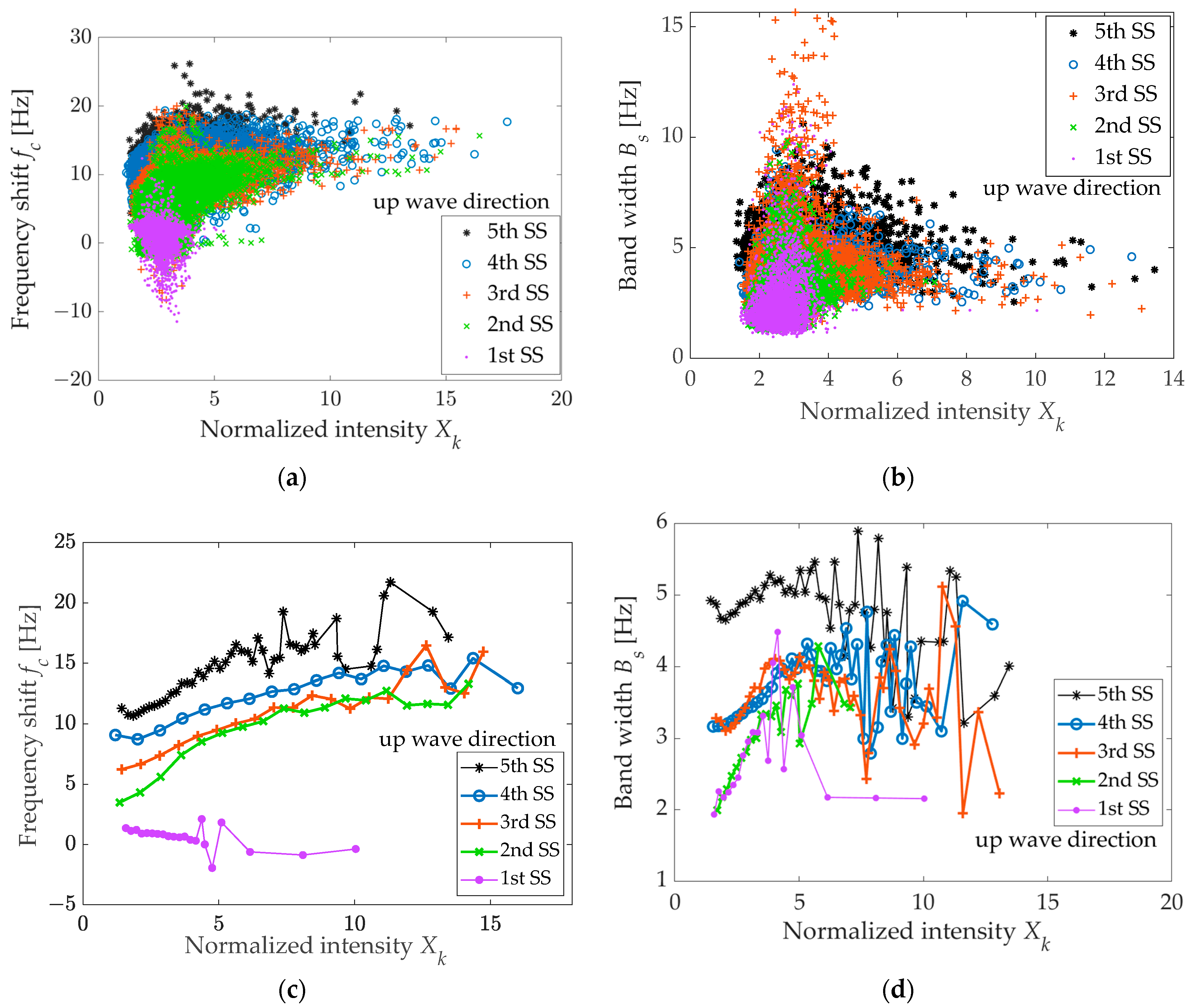
Jmse 11 01901 g017
Figure 18. Frequency shifts and bandwidths of short-time spectra depend on the normalized intensity of sea echoes in the up-wave direction. (a) Frequency shifts of data at different sea states. (b) Spectral widths of data at different sea states. Variation tendencies of (c) frequency shifts and (d) spectral widths.
Jmse 11 01901 g018
Figure 19. Frequency shift variation tendencies of short-time spectra with a normalized intensity of sea echo at different wave directions. (a) 4th, (b) 3rd, (c) 2nd, and (d) 1st sea states.
Jmse 11 01901 g019
Figure 20. Spectral width variation tendencies of short-time spectra with a normalized intensity of sea echoes at different wave directions. (a) 4th, (b) 3rd, (c) 2nd, and (d) 1st sea states.
Jmse 11 01901 g020
Figure 21. Variation tendencies of coefficients k and m with grazing angle θ . Calculated results of (a) coefficient g and (b) coefficient m . Markers represent calculated results, and lines represent CF.
Jmse 11 01901 g021
Figure 22. Model prediction results with data validation example. (a) 4.1° grazing angle in the up wave direction. (b) 5.6° grazing angle in the cross-wave direction with a relative angle of 20–40°. (c) 6.8° grazing angle in the cross-wave direction with a relative angle of 60–80°. Markers represent data, and lines represent model prediction results.
Jmse 11 01901 g022
Figure 23. Variation tendencies of coefficients n and t with grazing angle θ . Calculated results of (a) coefficient n and (b) coefficient t . Markers represent calculated results, and lines represent CF.
Jmse 11 01901 g023
Figure 24. Model prediction results with data validation example. (a) 0.7, (b) 0.9, and (c) 1.2 m SWH. Markers represent data, and lines represent model prediction results.
Jmse 11 01901 g024
Figure 25. Variation tendencies of frequency shift f s with normalized intensity X k in a mixed wave direction.
Jmse 11 01901 g025
Figure 26. Variation tendencies of frequency shift f s with normalized intensity X k in a mixed wave direction. Markers represent data, and lines represent model prediction results.
Jmse 11 01901 g026
Table 1. Radar parameters during measurement.
ParameterValue
PolarizationHH
PRF1000 Hz
Frequency456 MHz
Elevation angle−4°
Pulse width10 us (0.4 us compressed)
Resolution60 m
Height430 m
Grazing angles2° to 8°
Table 2. Oceanic parameters and definitions of relative wave or wind directions.
Oceanic ParametersValue
Wind speed w s (m/s)0.1–15
SWH h t (m)0.1–3.0
Wave/wind direction Δ φ (°)up wave/up wind ( 20 ° < Δ φ < 20 ° )
cross wave/cross wind ( 80 ° < Δ φ < 100 °   and 260 ° < Δ φ < 280 ° )
down wave/downwind ( 160 ° < Δ φ < 200 ° )
oblique-cross wave/wind (other values of Δ φ )
Table 3. Sea clutter datasets at each sea state in the Douglas standard.
Condition of Sea SurfaceParametersNumber of Datasets
Sea state1st1911
2nd5654
3rd1986
4th160
5th11
Wave directionup wave2252
down wave73
cross wave1044
oblique-cross wave6353
Table 4. Statistical occurrence probability of bimodal phenomenon.
Sea StatesProbability of Bimodal Spectra (%) S p 1 (dB) S p 2 (dB) F x 1 (Hz) F x 2 (Hz) F x (Hz)
1st sea stateUp wave22.6843.4337.280.98−1.955.49
Oblique-cross wave30.5844.1337.29−0.980.984.97
Cross wave27.0844.7836.001.910.105.20
2nd sea stateUp wave20.5246.2837.982.640.006.97
Oblique-cross wave21.1146.1936.860.721.145.96
Cross wave22.2846.9135.29−1.950.006.32
3rd sea stateUp wave7.9548.3238.025.4111.728.12
Oblique-cross wave4.7847.9845.112.313.296.25
Cross wave4.3647.6441.27−1.561.175.14
4th sea stateUp wave2.3555.1344.2011.2118.699.77
Oblique-cross wave1.1047.4840.616.1815.959.94
5th sea stateUp wave0.7463.5652.2912.8322.4211.87
Table 5. Fitting curve formula coefficients for frequency shifts and spectral widths with grazing angles.
Sea StatesFitting Curve Formula
f c = a θ + b B w = c θ + d
abcd
Up wave direction1st−0.111.19−0.656.23
2nd−0.212.59−0.394.93
3rd−0.507.73−0.274.81
4th−0.8113.79−0.144.18
5th−1.1618.50−0.0045.20
Table 6. Fitting curve formula coefficients for frequency shifts and spectral widths with SWHs.
Range   Bin   Number ,   θ (°) Wave   Direction ,   Δ φ (°)Fitting Curve Formula
f c = g h t + m B w = n h t + t
g m n t
60th range bin, 6.8°Up wave5.57−1.891.361.42
Cross wave (20–40°)4.37−1.471.361.42
Cross wave (40–60°)3.89−1.231.361.42
Cross wave (60–80°)2.52−1.870.841.41
Cross wave (80–90°)000.841.41
100th range bin, 4.1°Up wave7.51−2.480.842.75
Cross wave (20–40°)6.80−2.730.762.62
Cross wave (40–60°)5.91−1.780.582.66
Cross wave (60–80°)4.97−3.620.283.29
Cross wave (80–90°)000.192.84
Table 7. Fitting curve formula coefficients for frequency shifts and spectral widths with wind speed.
Range   Bin   Number ,   θ (°) Wind   Direction ,   Δ φ (°)Fitting Curve Formula
f c = r w s + p B w = u h t + q
r p u q
100th range bin, 4.1°up wave1.16−0.440.0553.39
oblique-cross wave0.42−0.710.0363.11
cross wave−0.24−2.03−0.183.93
down wave−3.582.020.0143.02
Disclaimer/Publisher’s Note: The statements, opinions and data contained in all publications are solely those of the individual author(s) and contributor(s) and not of MDPI and/or the editor(s). MDPI and/or the editor(s) disclaim responsibility for any injury to people or property resulting from any ideas, methods, instructions or products referred to in the content.

