Acoustic Field Radiation Prediction and Verification of Underwater Vehicles under a Free Surface

Abstract

This study aimed to examine the acoustic field radiated by propellers and underwater vehicles. For the verification of sound radiation in underwater vehicles, numerical methods are widely used in addition to experiments and propeller blade frequencies for calculation and validation. Numerical convergence and accuracy are more important for near-field and far-field problems. This paper uses the boundary element method (BEM) to assess the convergence of the finite volume method (FVM). In this study, the FVM, including the Reynolds-averaged Navier–Stokes method and the Ffowcs Williams–Hawkings (FW-H) acoustic model, is used to investigate the influence of various geometric inflows on the hydrodynamic and noise performance of the propeller. Then, the sound radiation of the FVM is compared with the BEM at the far field to determine the number of meshed elements. Furthermore, spectral analysis is being conducted to examine the noise generated by the underwater vehicle and propeller. The objective is to investigate the influence of the free surface on propeller efficiency. After verifying the numerical simulation, the results indicate that a relationship can be established between water pressure and propeller thrust under specific conditions. This relationship can be used to estimate the magnitude of propeller thrust at different water depths. The simulated results of propeller thrust, torque coefficient, propulsion efficiency, and sound radiation in this study are consistent with experimental values. This demonstrates the accuracy and practicality of the findings of numerical procedures in engineering applications.

1. Introduction

Requirements for vibration and noise reduction capabilities in propellers in modern marine engineering are increasing every year, particularly for underwater vehicles and naval vessels. The generation of noise is not only a standard for design inspection, but it also has serious consequences that can significantly impact the underwater environment and marine life. When an underwater vehicle travels at a constant speed, the surrounding water medium moves relative to the hull, creating a flow field around it. This flow field not only affects the hydrodynamic performance of underwater vehicles, but also generates low-frequency noise sources from propulsion propellers [1], particularly impacting the acoustic stealth of naval submarines. The noise sources of underwater vehicles mainly consist of mechanical noise, propeller noise, and hydrodynamic noise. Hydrodynamic noise is primarily generated by turbulent flow and pressure disturbances on the hull’s surface, as well as the interaction between appendages and turbulent pulsating pressure. However, when the underwater propeller reaches a certain speed, the boundary layer on its surface will generate turbulence and eddy current stripping. In more severe cases, cavitation may occur, causing the surface to rupture and radiate strong noise. When sailing at low speed, the proportion of hydrodynamic noise to underwater hull-radiated noise is much lower than that of mechanical and propeller noise. Due to the generation of these noises, some technical sonar and other instruments [2,3] were developed. Therefore, the impact of these noise sources is also significant, and can no longer be ignored.

Traditionally, the performance of underwater vehicles and propellers was studied based on the results obtained from open water testing. However, this approach is limited by cost and issues with experimental accuracy [4,5]. In recent years, with the advancement of computational power in computers, computational fluid dynamics (CFD) became the predominant method for calculating flow fields. The shear stress transport (SST) k-ω turbulence model, proposed by Menter [6] and combined with the FVM, was extensively utilized in research [7,8,9]. To more accurately calculate the influence of the free surface, Hirt and Nichols [10] introduced the volume of fluid method (VOF), which was subsequently widely adopted by researchers [11,12,13,14]. This method became the primary computational technique for analyzing two-phase flow, particularly involving free surfaces. Califano and Steen [11] simulated the changes in the thrust and torque of a propeller as it approaches the free surface with air ventilation. Paik [12] built upon existing research and studied the fluid dynamic characteristics of propellers under the free surface. This study further confirmed that these characteristics depend on depth, model size, and advance ratio. Subsequently, Eom et al. [13,14] pointed out that under a fixed advance ratio, thrust and water depth exhibit a linear relationship. Furthermore, Cianferra and Armenio [15] conducted a dimensional analysis. They found significant errors in their observations of full-scale acoustic pressure from reduced-scale models under free surface conditions in the far field. Therefore, when utilizing a numerical model under the free surface, we not only consider the influence of reduced-scale dimensions, but also take into account the effects of thrust and water depth.

When investigating underwater noise problems, researchers often utilize the inhomogeneous wave equation derived from the Lighthill equation to determine the field of radiated noise [16,17,18]. However, when underwater vehicles approach the water’s surface, they are influenced by the free surface. This can result in a decrease in thrust and potentially impact propeller noise [19,20]. Therefore, using numerical models, it is necessary to study the impact of the free surface on underwater vehicles with propellers. In this paper, we verified the model using the experimental results of Choi [8] and simulated the flow field of a submarine using the SST k-ω turbulence model. Additionally, the BEM was used to verify the convergence of the meshes of FVM for calculating radiated acoustic pressure in the far-field sound radiation. Finally, the VOF method was used to investigate the propeller’s performance in the presence of a free surface. As a result, we were able to establish a formula that relates thrust to water depth [13,14]. In recent years, some scholars [21,22,23] used acoustics to predict the radiated noise of marine propellers. The findings of this study can be used for the identification of sound sources, determining the distance between the free surface and the propeller, and estimating the magnitude of propeller thrust at various water depths.

2. Theoretical Foundations

This study utilizes CFD numerical simulations to analyze the steady-state and transient theoretical acoustic fields of underwater propellers. The basic theories used include Reynolds-averaged Navier–Stokes equations, turbulence models, acoustic theory, and the VOF method, which are described as follows.

2.1. Reynolds-Averaged Navier–Stokes Equations (RANS)

Reynolds-averaged Navier–Stokes equations are used to solve equations for time-averaged turbulent flow. The equations represent a combination of instantaneous momentum and time-averaged flow quantities, and can be written as shown in Equations (1) and (2):

$$\frac{\partial \rho }{\partial t}+\frac{\partial }{\partial x_i}\left(\rho u_i\right)=0,$$

(1)

$$\frac{\partial }{\partial t}\left(\rho u_i\right)+\frac{\partial }{\partial x_j}\left(\rho u_i{u}_j\right)=\frac{\partial p}{\partial x_j}+\frac{\partial }{\partial x_j}+(\mu \frac{\partial u_i}{\partial x_j}-\rho \overline{u_i^{’}{u}_j^{’}})+S_j,$$

(2)

where ρ represents fluid density, $u_i$ denotes the time-averaged value of the velocity component, p is the time-averaged value of pressure, μ is the fluid dynamic viscosity coefficient, $\rho \overline{u_i^{’}{u}_j^{’}}$ is the Reynolds stresses’ term, and $S_j$ is the generalized source term.

Generally, using time-averaged properties to describe the flow’s physical behavior is suitable for most engineering purposes; the numerical simulation of time-averaged turbulent flow equations provides accurate results. However, when using direct numerical simulation or the large eddy simulation method, the sizes of the vortices and turbulent scales both decrease, leading to higher computational costs. For most engineering purposes, this makes the process impractical. Therefore, the RANS method became a more effective and feasible means of utilizing various turbulence models to analyze vortex phenomena.

2.2. SST k-ω Turbulence Model

The SST k-ω turbulence model, proposed by Meter [6], combines the advantages of Wilcox’s k-ω model [24], which provides higher computational accuracy for wall effects, and Launder’s k-ε model [25], which converges well for average flow. The turbulence model proposed by Meter can automatically switch between wall functions or the low Reynolds formulation [26,27] depending on the distance between the calculation point and the wall. The equations for turbulent kinetic energy (k) and specific dissipation rate (ω) are represented by Equations (3) and (4):

$$\frac{\partial \left(\rho k\right)}{\partial t}+\frac{\partial \left(\rho k{u}_i\right)}{\partial x_i}=\frac{\partial }{\partial x_j}\left[{\mathsf{\Gamma }}_k\frac{\partial k}{\partial x_j}\right]+\widetilde{{\mathrm{G}}_k}-{\mathrm{Y}}_k+{\mathrm{S}}_k,$$

(3)

$$\frac{\partial \left(\rho \omega \right)}{\partial t}+\frac{\partial \left(\rho \omega u_i\right)}{\partial x_i}=\frac{\partial }{\partial x_j}\left[{\mathsf{\Gamma }}_{\omega }\frac{\partial \omega }{\partial x_j}\right]+{\mathrm{G}}_{\omega }-{\mathrm{Y}}_{\omega }+{\mathrm{S}}_{\omega },$$

(4)

where ${\mathsf{\Gamma }}_k$ and ${\mathsf{\Gamma }}_{\omega }$ are the diffusion terms for k and ω, $\widetilde{{\mathrm{G}}_k}$ is the production of turbulent kinetic energy due to mean velocity gradients, and ${\mathrm{G}}_{\omega }$ is the dissipation rate generation term. Y_k and Y_ω are the generation and dissipation terms of turbulence, respectively, and S_k and S_ω is a user-defined source term.

2.3. Lighthill Acoustic Analogy

Lighthill derived the Lighthill acoustic analogy [28,29] by using Navier–Stokes equations in the study of excitation experiments of jet and free turbulent sound.

The Lighthill equation can be expressed as follows in Equation (5):

$$\frac{1}{c_0^2}\frac{{\partial }^2\left(\rho -{\rho }_0\right)}{\partial t^2}-{\nabla }^2\left(\rho -{\rho }_0\right)=\nabla \cdot \nabla {\mathrm{T}}_{ij},$$

(5)

$${\mathrm{T}}_{ij}=\rho u_i{u}_j-{\tau }_{ij}+{\delta }_{ij}\left[\left(P{-P}_0\right)-c_0^2\left(\rho -{\rho }_0\right)\right],$$

(6)

where T_ij is the Lighthill turbulent stress tensor, $c_0^{}$ is the speed of sound in the medium, and u_iu_j represents the Reynolds stress. According to the Lighthill analogy, Equation (6) includes the effects of the turbulent stress tensor, which consists of Reynolds stress induced by velocity, fluid–fluid viscous stresses, and thermal conduction. In this paper, since the viscous stress between the fluids in turbulent flow is negligible, the calculation assumes an ideal fluid with a low Mach number, relative motion, and adiabatic and isentropic processes. Hence, the Lighthill turbulent stress tensor is represented as Equation (7):

$${\mathrm{T}}_{ij}=\rho u_i{u}_j.$$

(7)

2.4. Ffowcs Williams–Hawkings Acoustic Analogy

The FW-H equation [30], itself based on the use of a free-space Green’s function, is the basis of the Lighthill equation used to derive the sound wave equation generated by moving objects. It is a form of inhomogeneous wave equation, including continuity and momentum equations, even when considering the surface of integration in the nonlinear flow region. In this study, the FW-H acoustic analogy model is used to predict small-amplitude acoustic pressure fluctuations in the far field, using near-field flow data from a CFD solution. Therefore, the FW-H acoustic model can be used for the numerical simulation of the sound radiation of submarines and propellers in this study. The inhomogeneous wave FW-H equation is represented by Equation (8).

$$\begin{array}{ll}\frac{1}{c_0^2}\frac{\partial \left(\rho -{\rho }_0\right)}{\partial t^2}-{\nabla }^2\left(\rho -{\rho }_0\right)& =\frac{\partial }{\partial t}\left\{\left[{\rho }_0{v}_n+\rho \left(u_n-v_n\right)\right]\delta \left(\mathrm{f}\right)\right\}+\frac{{\partial }^2}{\partial x_i\partial x_j}\left\{T_{ij}H\left(\mathrm{f}\right)\right\}\\ & -\frac{\partial }{\partial x_i}\left\{\left[P_{ij}{n}_j+\rho u_i\left(u_n-v_n\right)\right]\delta \left(\mathrm{f}\right)\right\},\end{array}$$

(8)

$$P_{ij}=p{\delta }_{ij}-\mu \left(\frac{\partial u_i}{\partial x_j}+\frac{\partial u_j}{\partial x_i}-\frac{2}{3}\frac{\partial u_k}{\partial x_k}{\delta }_{ij}\right),$$

(9)

where $u_i$ represents the fluid velocity component in the $x_i$ direction. $u_n$ and $v_n$ are the fluid velocity component perpendicular to the integration plane and moving velocity component of the integration plane. $\delta \left(\mathrm{f}\right)$ is the Dirac function, $H\left(\mathrm{f}\right)$ is the Heaviside function, and P_ij is the compressible stress tensor, as shown in Equation (9). Equation (8) includes a term for a monopole sound source located at the determined quadrupole sound sources, which are distributed throughout the stress variation of the flow field. The other two terms are surface sound sources, namely the dipole sound source caused by the perpendicular stress of the fluid and the monopole sound source caused by variations in velocity and thickness.

2.5. Volume of Fluid Method

The volume of fluid (VOF) method was first proposed by Hirt and Nichols [10] as a method for capturing the wave motion between two-phase fluids. It utilizes an equivalent fluid approach to interpolate the physical properties, such as density and viscosity, of the equivalent fluid based on the volume fraction C. The definition of C is provided by Equation (9), and is related to the fluid density and viscosity as defined by Equations (10) and (11), respectively:

$$C={\mathrm{V}}_{\mathrm{w}\mathrm{a}\mathrm{t}\mathrm{e}\mathrm{r}}/{\mathrm{V}}_{\mathrm{c}\mathrm{e}\mathrm{l}\mathrm{l}},$$

(10)

$$\rho =C{\rho }_{\mathrm{w}\mathrm{a}\mathrm{t}\mathrm{e}\mathrm{r}}+(1-C){\rho }_{\mathrm{a}\mathrm{i}\mathrm{r}},$$

(11)

$${\mu }_t=C{\mu }_{water}+(1-C){\mu }_{air},$$

(12)

where V_cell is the control volume, V_water is the volume occupied by water in the control volume, ρ is the density, and ${\mu }_t$ is the viscosity. The fluid type of the mesh in the calculation domain can be defined according to the ratio of the two phases, which is defined as follows:

$$C=\left\{\begin{array}{cc}1,& \mathrm{w}\mathrm{a}\mathrm{t}\mathrm{e}\mathrm{r}\\ 0,& \mathrm{a}\mathrm{i}\mathrm{r}\\ 0<C<1,& \mathrm{t}\mathrm{r}\mathrm{a}\mathrm{n}\mathrm{s}\mathrm{i}\mathrm{t}\mathrm{i}\mathrm{o}\mathrm{n}\mathrm{r}\mathrm{e}\mathrm{g}\mathrm{i}\mathrm{o}\mathrm{n}\end{array}\right..$$

(13)

3. Simulation and Verification of the Propeller

To explore the influence and rationality of propeller rotation on the radiated sound field, this study uses ANSYS Fluent v19 to analyze and solve the flow field. For equations related to the BEM acoustic theory, please refer to the LMS Virtual Lab [31]. Comparing the numerical simulation value of the model with the experimental value in [9], it is verified that the numerical simulation result, propeller thrust, torque coefficient, and propulsion efficiency are the same as the experimental values. Then, by calculating the time-domain solution of the FVM, and using the LMS Virtual Lab [31] to calculate the frequency-domain solution of the BEM, at the far field, the two acoustic pressures are the same.

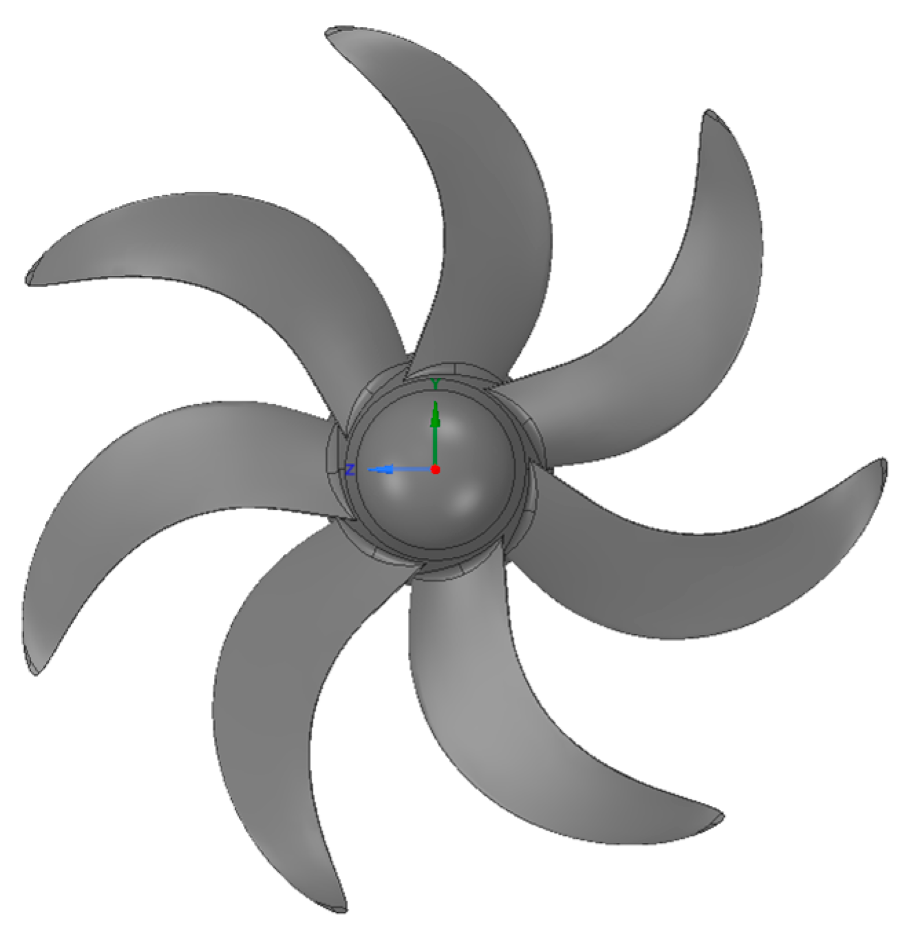
3.1. Geometric Model

In this study, an INSEAN E1619 seven-blade propeller was used as the computational model for the numerical simulation. The experimental values in reference [9] were obtained through laser Doppler velocimetry (LDV). The geometric model of the propeller is shown in Figure 1, and the propeller parameters are shown in

Table 1. Geometric parameters of the E1619 propeller model.

Description	Symbol	Parameters
Number of blades	B	7
Propeller diameter (m)	D	0.485
Pitch ratio at 0.7R	P0.7/D	1.15
Hub ratio	Dh/D	0.226
Chord length at 0.75R (m)	C0.75	0.0068
Expansion area ratio	Ag/A	0.608

.

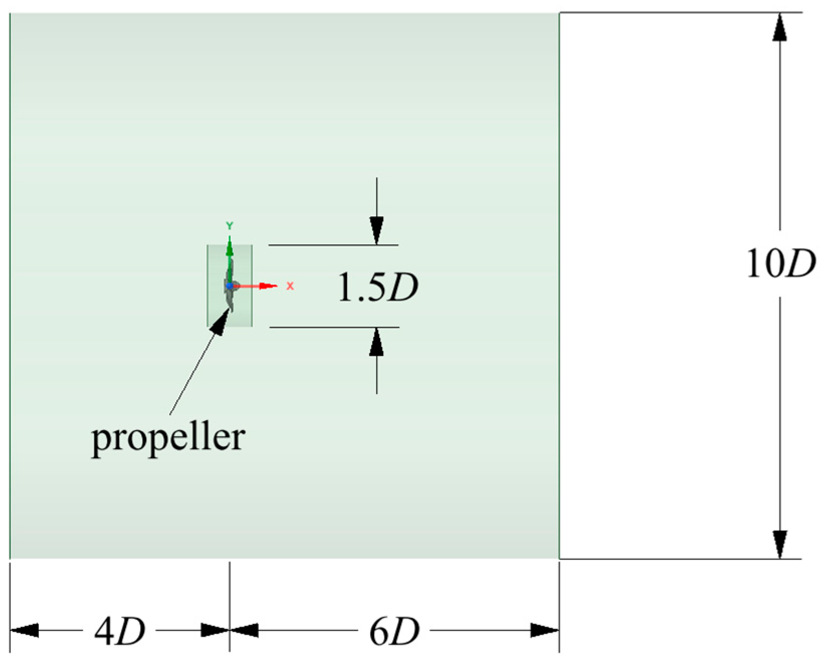
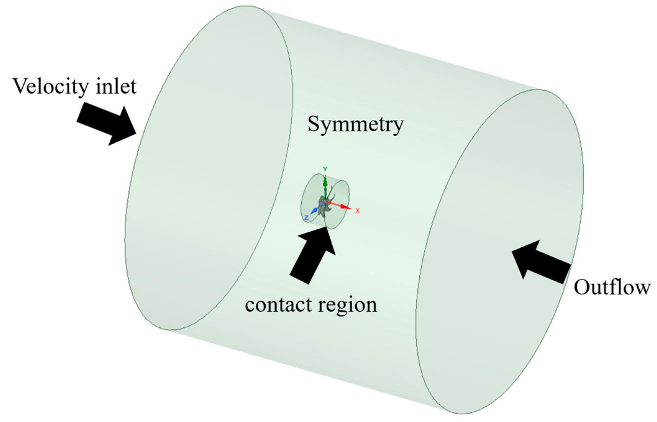
3.2. Setting Boundary Conditions for the Propeller Model

The coordinate system and boundary conditions of the calculation domain are set as shown in Figure 2 and Figure 3. In the self-propulsion simulation, the rotating domain of the propeller is a cylinder whose center is the center of the propeller, and its diameter is 1.5 times the diameter of the propeller as shown in Figure 2. In Figure 3, the fluid flow on the left boundary condition remains in a uniform flow state until it is exposed to the internal flow field. Since the main focus of this study is the extension of the wake, the distance from the fluid inlet to the inner flow field is reduced, while the distance from the inner flow field to the fluid outlet is increased. The fluid inlet is set as a velocity inflow (velocity inlet), and the outlet is set as an outflow (outflow). To eliminate the influence of the boundary face, the area around the calculation domain adopts the symmetric boundary condition (symmetry) [32], where the normal gradient of the surface is zero. In order to ensure that discontinuous meshes can still facilitate the transfer of values, a sliding boundary condition [33] (sliding boundary condition) is established between the internal and external flow fields.

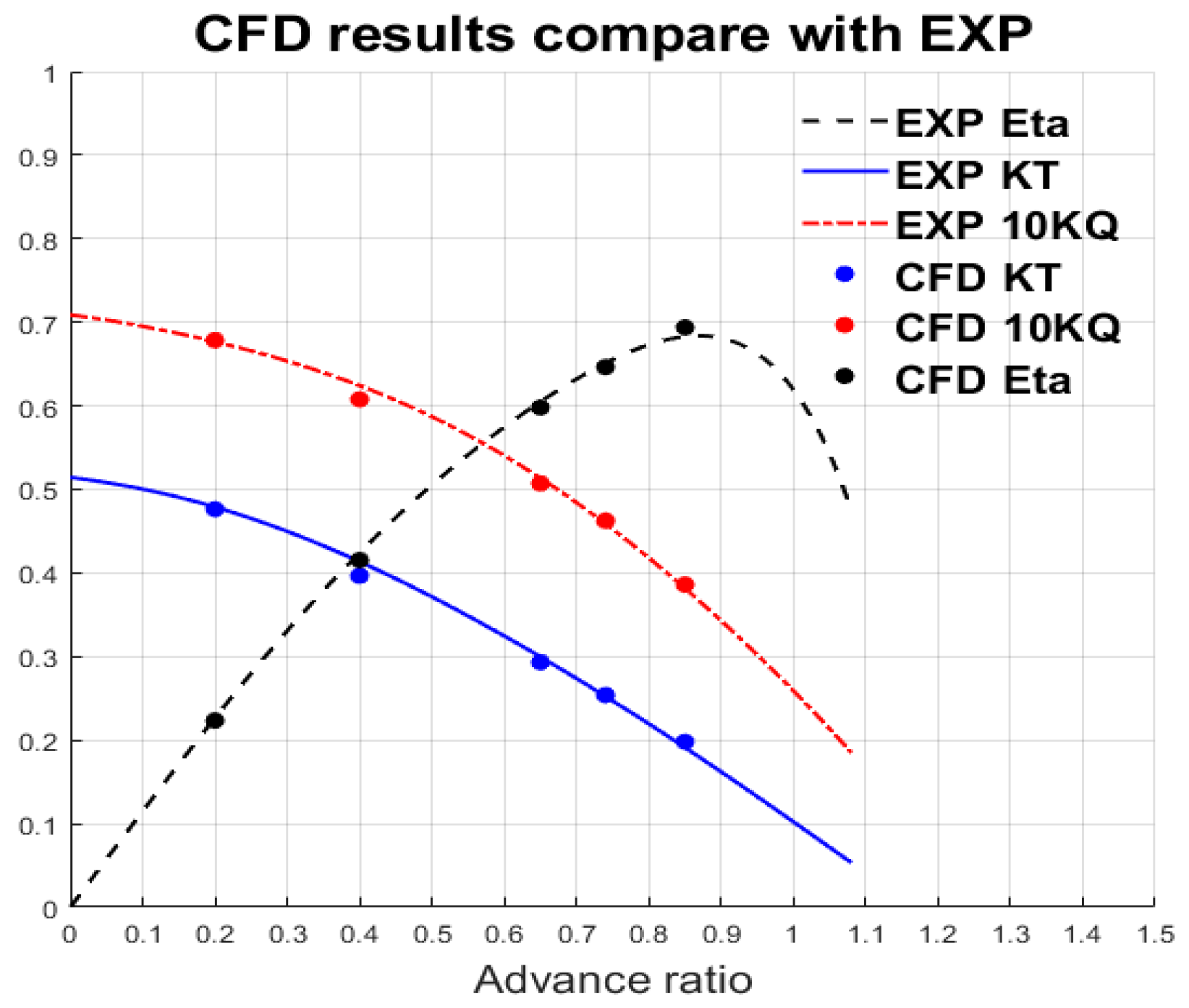
3.3. Propeller Performance Verification

In this section, the results of the numerical simulation calculations are compared and verified with the experimental values of the open water test in [9]. The incompressible fluid is considered in the numerical experiments of this study. The parameters are listed as follows: the fluid density (ρ) and sound velocity ($c_0^{}$) are set at ρ = 998 kg/m³ and $c_0^{}$= 1500 m/s. The inflow velocity ($U_{\infty }$) is 1.68 m/s. The formulas for thrust, torque, and propulsion efficiency are expressed as follows:

$$J=U_{\infty }/nD,$$

(14)

$$K_T=T/{\rho n}^2{D}^4,$$

(15)

$$K_Q=Q/{\rho n}^2{D}^5,$$

(16)

$$\eta =\frac{K_T}{K_Q}\times \frac{J}{2\pi },$$

(17)

where J is the advance ratio, n is the propeller speed, D is the diameter, K_T is the thrust coefficient, T and Q are the thrust and torque obtained from the numerical simulation, respectively, ρ is the density, K_Q is the torque coefficient, and η is the propulsion efficiency.

This study used a total mesh count of 8.53 million, as shown in Figure 4. Five different advance ratios (J), 0.85, 0.74, 0.65, 0.4, and 0.2, were used as comparative validation benchmarks. After the thrust and torque values caused by propeller rotation reached a stable state, they were converted to dimensionless coefficients K_T, K_Q, and η for comparison with the experimental values from reference [9], as shown in

Table 2. Comparison of experimental and simulation values of thrust and torque coefficient.

INSEAN E1619		EXP.	CFD	Diff.
0.85 J	KT	0.196	0.1995	1.78%
	10KQ	0.388	0.3875	−0.12%
0.74 J	KT	0.250	0.2539	1.56%
	10KQ	0.450	0.4626	2.80%
0.65 J	KT	0.302	0.2932	−2.90%
	10KQ	0.515	0.5072	−1.52%
0.4 J	KT	0.412	0.3966	−3.70%
	10KQ	0.621	0.6078	−2.19%
0.2 J	KT	0.481	0.4764	−0.97%
	10KQ	0.680	0.6785	−0.17%

. The numerical simulation results from Table 2 are plotted against the experimental values in Figure 5. The results show that the maximum relative deviation is 3.7%, and there is good agreement between the numerical simulations and experimental trends, as shown in Figure 5. Figure 6 shows the pressure distribution diagram of the thrust surface and resistance surface of the propeller at 0.85 J. It can be seen from the figure that the pressure on the thrust surface increases from the blade root to the blade tip, and the surface resistance reduces from the blade root to the blade tip. Since the pressure on the thrust surface of the propeller is greater than that on the resistance surface, a propulsion effect is produced. The numerical simulation results in Table 2 and the experimental values are plotted in Figure 5, from which it can be seen that the numerical simulation results are consistent with the experimental trends.

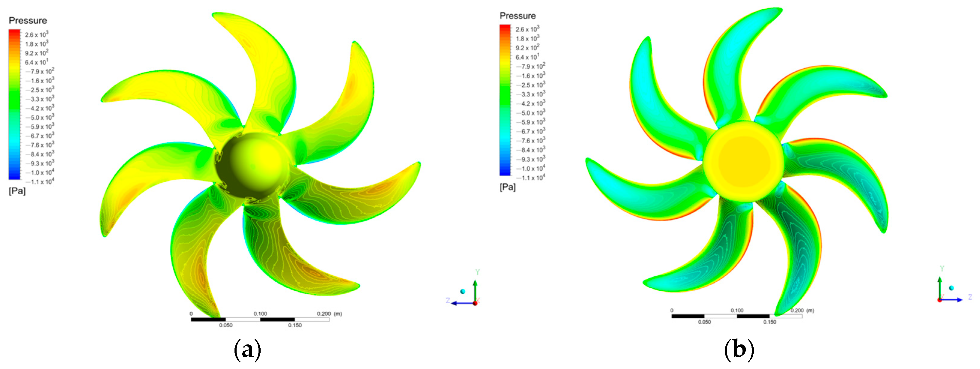
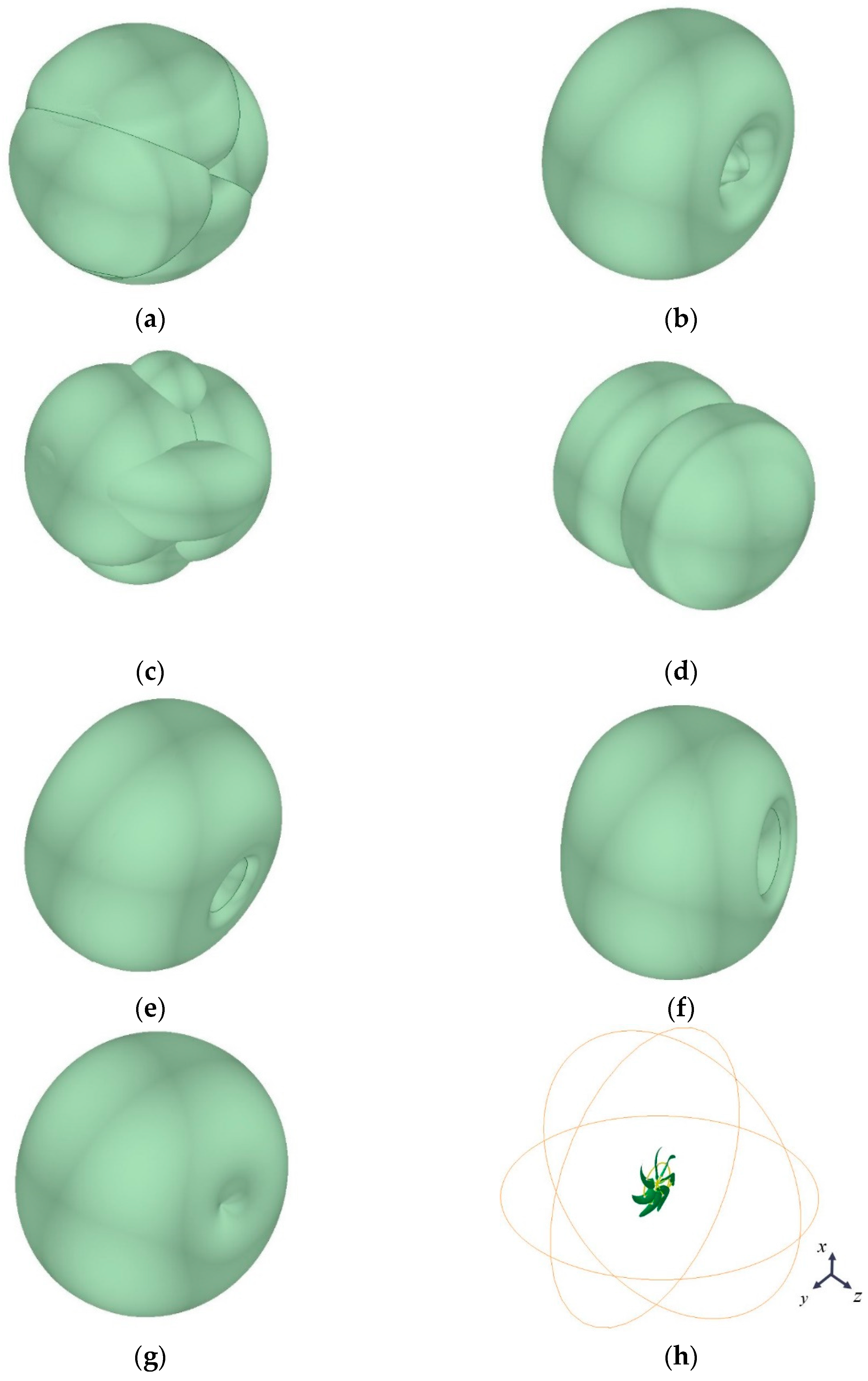
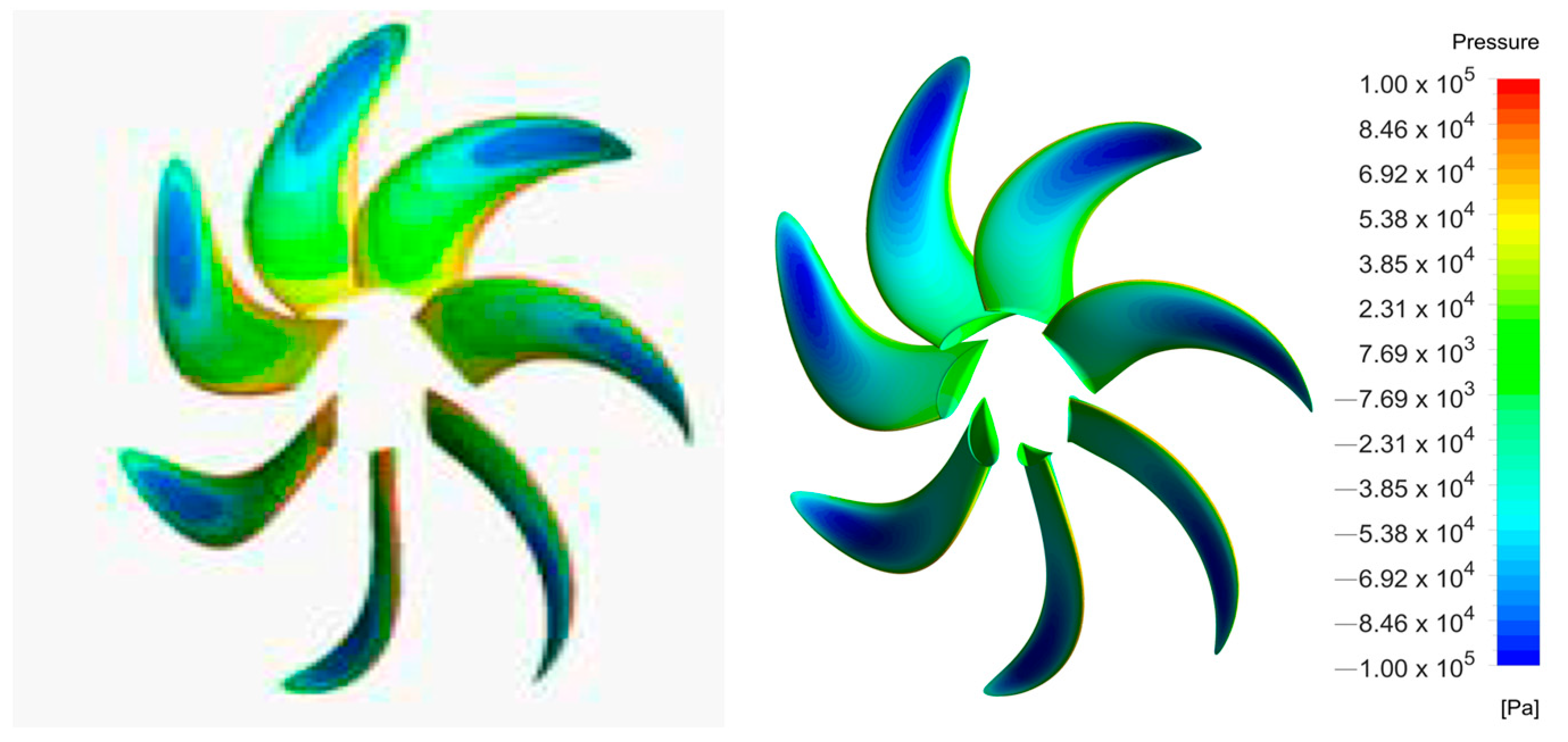
3.4. Calculation and Analysis of the Sound Field Radiation of the Propeller

CFD calculations were performed in order to obtain values of time-domain pressure pulsations on the surface of the propeller blades. These pressure pulsations were combined with the FW-H acoustic analogy model to find the acoustic pressure, itself obtained from the solution of FVM and of BEM. The consistency of the results obtained using the two methods was verified. In this study, the measurement points for the sound field points were set at distances of 1D, 2.5D, 5D, and 10D in both the radial and axial directions of the propeller. These points are illustrated in Figure 7, with the geometric center of the propeller serving as the origin. The pressure values measured at each measurement point were converted to the sound pressure level (SPL), and the blade passing frequency (BPF) of the propeller was used as a reference for comparison, as shown below.

$$\mathrm{d}\mathrm{B}=20\mathrm{l}\mathrm{o}\mathrm{g}\left(\frac{P_{rms}}{P_{ref}}\right),$$

(18)

$$f_b=m\times B\times n,$$

(19)

where P_rms is the root mean square value of acoustic pressure. P_ref is the reference acoustic pressure value, calculated as ${10}^{-6}$ Pa in water. Here, B represents the number of blades, m = 1, 2, 3…, and B_N, respectively, represents the frequencies of the first to B_N blades; and n represents the number of revolutions per second of the propeller (rps).

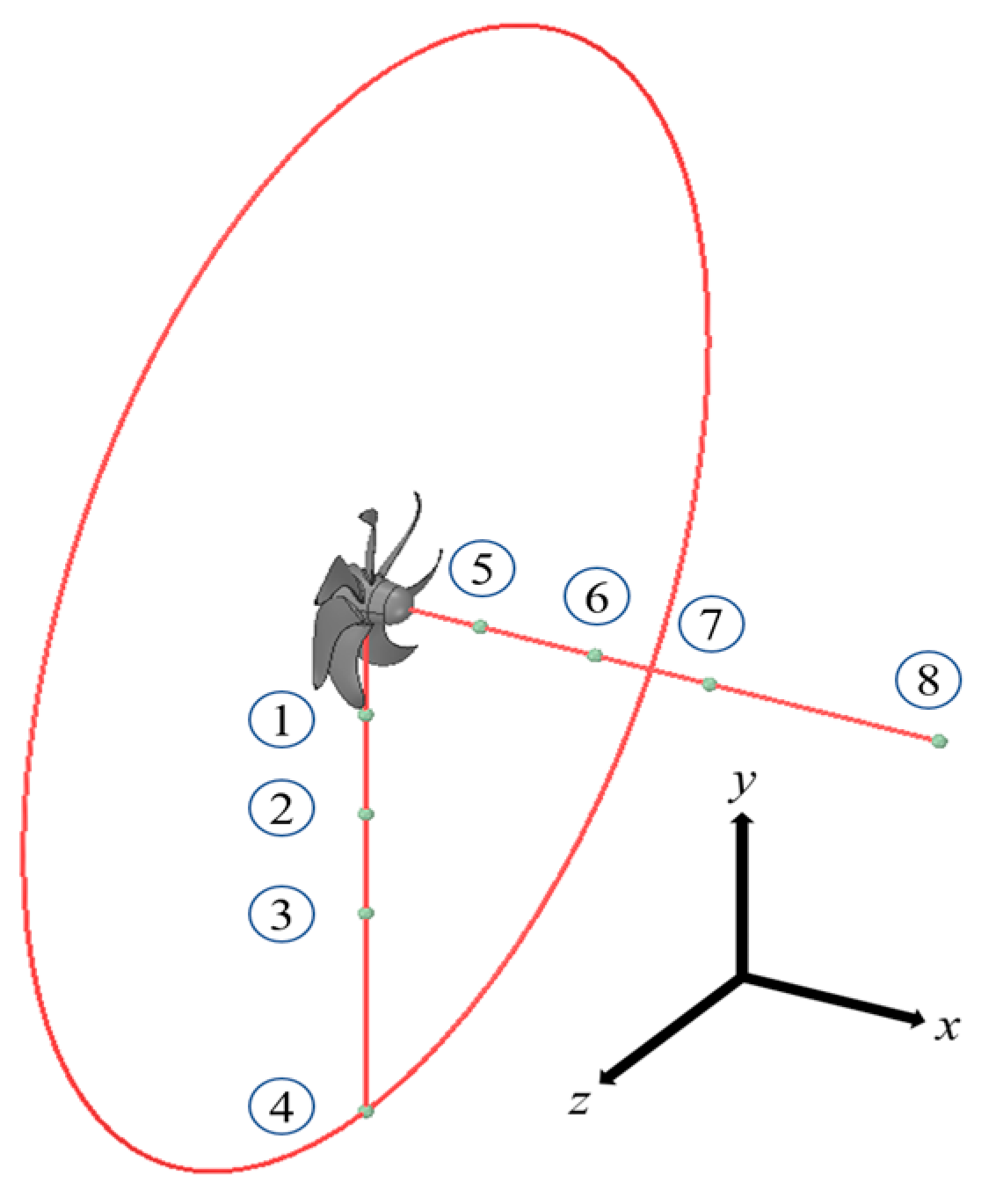
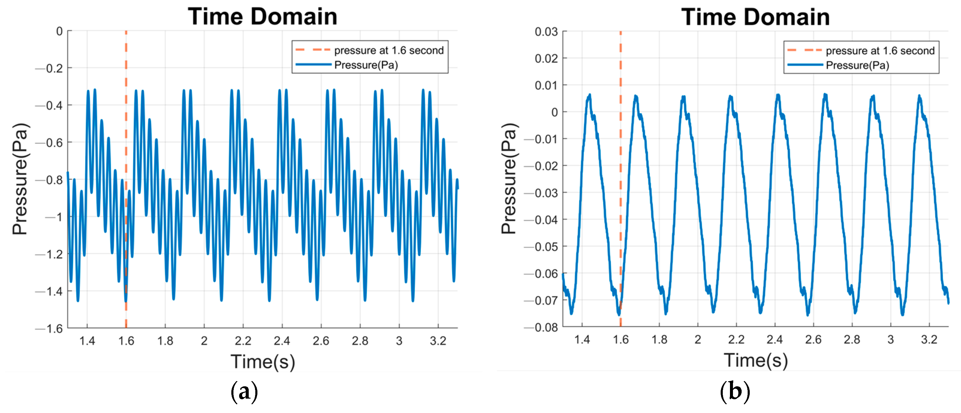
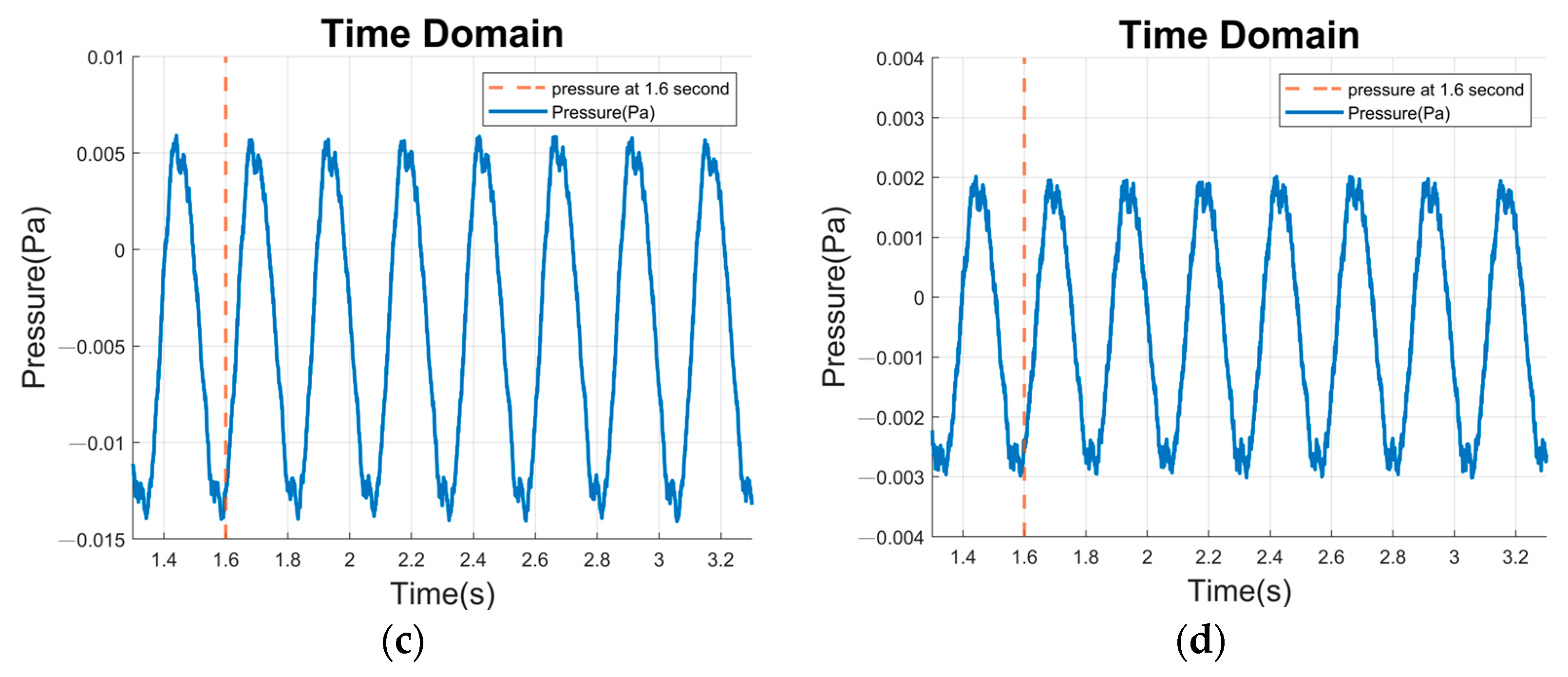
3.5. Sound Field Radiation Verification

Within the analysis of propeller-radiated noise in the sound field, first, the FVM is used to solve the pressure fluctuations of the propeller, and the FW-H acoustics model is then used to calculate the radiated noise in the far field. These fluctuations are utilized in a fast Fourier transform (FFT), which is converted into spectral noise in the frequency domain. Then, the propeller blade surface’s pressure fluctuation, which is calculated using CFD (ANSYS 2022R1), is applied with the BEM. It converts the pressure fluctuation into a dipole sound source, which serves as the boundary condition for the BEM. Since the BEM automatically satisfies the fundamental solution of the sound field when calculating the far field, it does not require a large number of meshes. According to the far-field conditions, the results of the BEM can be used to ensure mesh convergence for the FVM. Thus, using this numerical procedure, the convergence of the sound field calculation results is accelerated.

In this section, the following working conditions are set: an advance ratio of 0.85 J, a fluid inflow velocity of 1.68 m/s, and a propeller rotational speed of 4.0752 rps. The first blade frequency of the propeller at this stage is 28.5264 Hz. The sampling time is 6.8163 × 10⁻⁴ s. The time-domain pressure pulsations of each field point in the radial and axial directions are represented by the absolute value of the pressure, respectively, as shown in Figure 8 and Figure 9. The absolute values of the pressure at each field point in the radial and axial directions at a time of 1.6 s are shown in Figure 10 and Figure 11. To conduct acoustic qualitative verification, the pressure value at the field point decreases in inverse proportion to the distance from the origin, and the acoustic pressure tends to zero at the far field. This phenomenon conforms to the acoustic description of the solution for an infinite sound field.

Comparisons with the acoustic pressure at the different field points of FVM and the BEM are shown in Figure 12 and Figure 13. From the numerical results at 10D, it can be found that the trend in the acoustic pressure of BEM can be used to effectively approximate the result of FVM. Further quantitative analysis from Figure 12 and Figure 13 shows the pressure of the different field points in the radial and axial directions in

Table 3. Comparison of received acoustic pressure at radial field points.

	FVM	BEM	Diff.
4.0752 Hz
Point 1	108 (dB)	105.8 (dB)	2.2 (dB)
Point 2	91.59 (dB)	89.74 (dB)	1.85 (dB)
Point 3	79.49 (dB)	77.69 (dB)	1.8 (dB)
Point 4	67.46 (dB)	65.66 (dB)	1.8 (dB)
28.5264 Hz
Point 1	109.1 (dB)	91.41 (dB)	17.69 (dB)
Point 2	61.65 (dB)	59.56 (dB)	2.09 (dB)
Point 3	50.38 (dB)	48.65 (dB)	1.73 (dB)
Point 4	39.52 (dB)	37.68 (dB)	1.84 (dB)

and

Table 4. Comparison of received acoustic pressure at axial field points.

	FVM	BEM	Diff.
16.3008 Hz
Point 5	81.73 (dB)	80.03 (dB)	1.7 (dB)
Point 6	66.34 (dB)	64.61 (dB)	1.73 (dB)
Point 7	54.34 (dB)	52.66 (dB)	1.68 (dB)
Point 8	42.59 (dB)	40.93 (dB)	1.66 (dB)
32.6016 Hz
Point 5	81.89 (dB)	81.88 (dB)	0.01 (dB)
Point 6	66.32 (dB)	67.06 (dB)	0.74 (dB)
Point 7	54.73 (dB)	55.54 (dB)	0.81 (dB)
Point 8	43.98 (dB)	44.68 (dB)	0.7 (dB)

. As shown in Figure 12 and Table 3, the maximum radial pressure at the near and far field occurs at 4.0752 and 28.5264 Hz; similarly, the maximum axial pressure at the near and far field occurs at 16.3008 and 32.6016 Hz. The maximum deviation is 17.69 (dB), as calculated by the BEM, and occurs at the first blade frequency of the propeller. As mentioned, all excitation frequencies are excited by the rotational angular velocity, which may prove the accuracy of this numerical procedure.

For sound field directivity, the acoustic pressure transfer under different excitation frequencies (4.0752, 8.1504, 12.2256, 16.3008, 20.376, 24.4512, and 28.5264 Hz) presented in three-dimensional form, as shown in Figure 14. As shown in Figure 14c, at 12.2256 Hz, the coupling superposition model of the thrust and torsional sound wave is similar. Likewise, the energy at 16.3008 Hz mainly transmitted along the direction of the rotating shaft, as shown in Figure 14d. Within propeller theory, the superposition of thrust and torsion sound wave energy presents different patterns at different frequencies, as shown in Figure 14a–g. This phenomenon is caused by the spiral detachment noise formed by the superposition of the axial inflow and propeller thrust. In addition, the sound energy at 12.2256 and 16.3008 Hz is transmitted in the direction of the rotating axis, and at other frequencies, it is transmitted in the radial direction. This phenomenon is known as axial inflow and propeller thrust. The vortex formed by the superposition is free of noise. Except for the sound energy at the two frequencies mentioned above, which transmitted in the direction of the rotation axis, the transmission of sound energy at other frequencies is primarily in the radial plane.

4. Analysis of the Radiation Sound Field of Underwater Vehicles

In this section, the DARPA SUBOFF model of the underwater vehicle is combined with the INSEAN E1619 model to conduct a simulation test of the radiation sound field during a self-propulsion experiment using the underwater vehicle. The results will be compared with the results of the cavitation tank experiment [8] to verify their numerical accuracy.

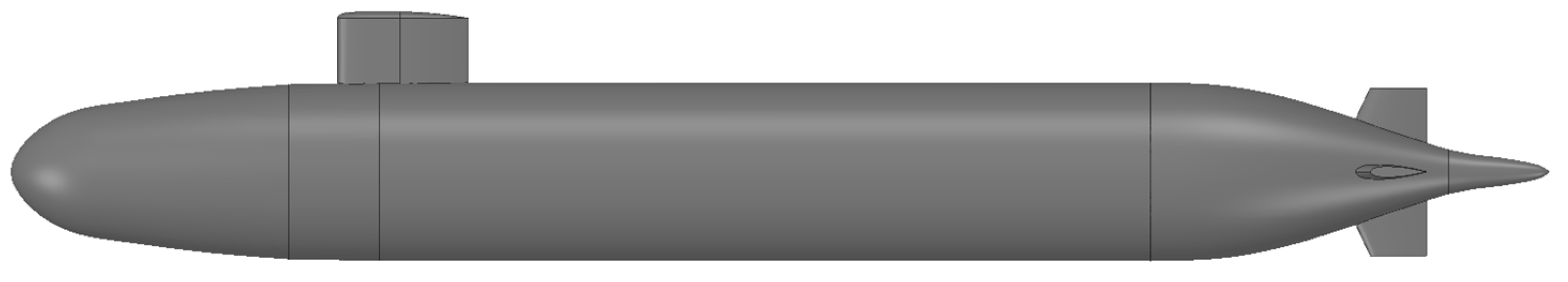
4.1. Geometric Model Studied

This section utilizes the DARPA SUBOFF model [4] as an underwater vehicle for verification. The SUBOFF model features a cross-shaped hull (AFF8+), and its geometric parameters and model are displayed in Figure 15 and

Table 5. Primary parameters of DARPA SUBOFF.

Description	Symbol Flag	Parameters
Overall length	LOA	4.356 m
Vertical mark spacing	LPP	4.261 m
Maximum hull radius	Rmax	0.254 m
Center of buoyancy	FB	0.254 LOA
Drainage volume	Vdisp	0.718 m3
Wet cut-off area	SW	6.338 m2

.

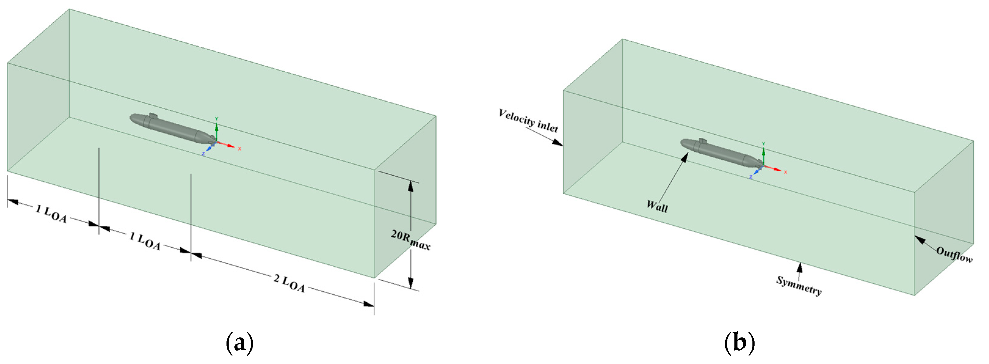
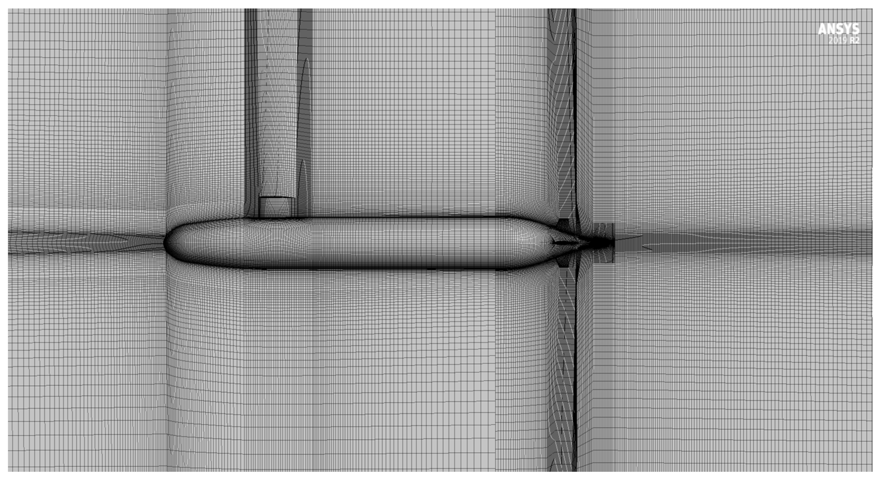
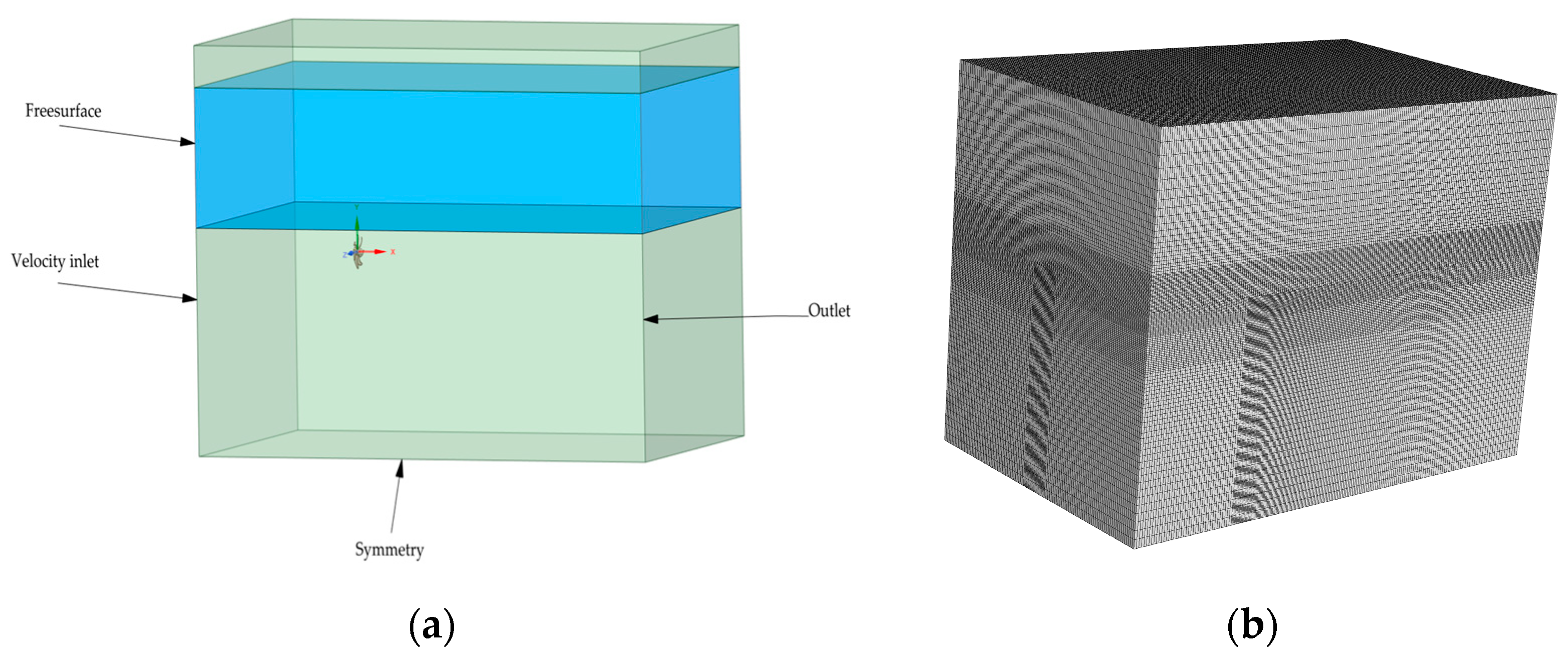
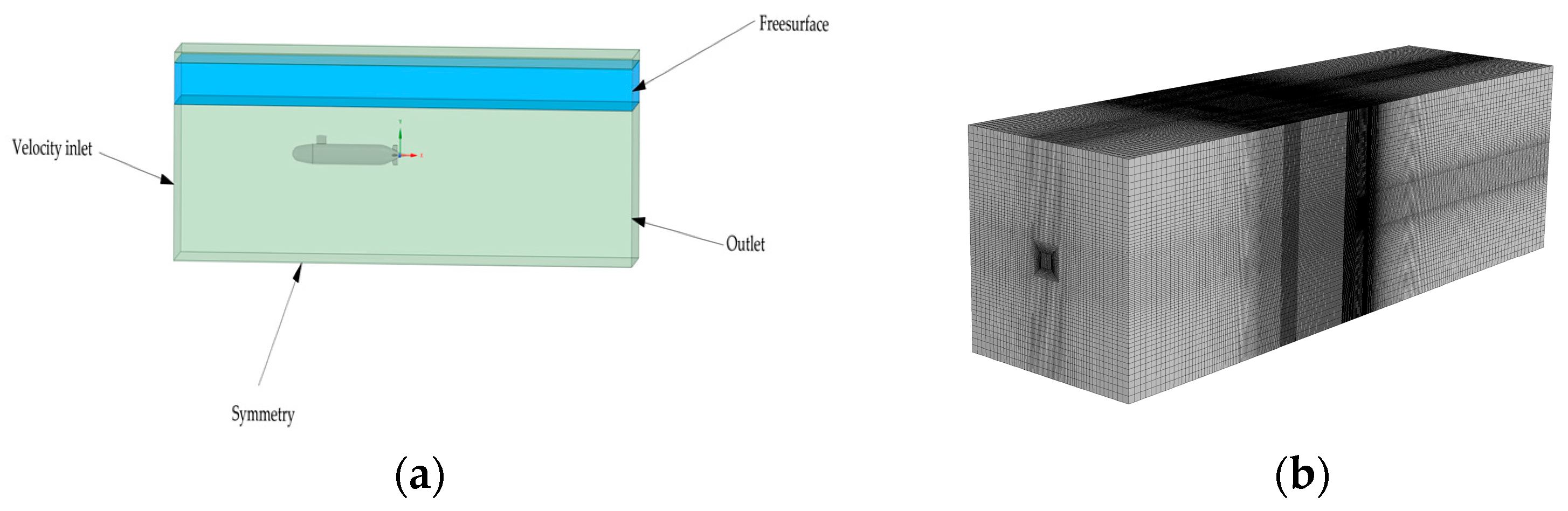
4.2. Boundary Condition Setting for the Underwater Vehicle

In this section, the hull model is combined with the INSEAN E1619 to simulate a self-propulsion test using underwater vehicles. The experimental settings of the large cavitation tunnel (LCT) and the results from the literature [9] are used as a basis for comparison. Since the original size of the propeller is 0.485 m, which differs from the actual length of the hull used in the self-propulsion test, the propeller’s diameter scales to 0.262 m during the verification process. According to the literature [32,33], the coordinate system and boundary conditions of the calculation domain are set as shown in Figure 16. The calculation domain of the external geometry and the submarine’s hull geometry are shown in Figure 16a. Here, L_OA is the overall length of the submarine, and R_max represents the maximum radius of the hull. The height is set to 20 times the maximum hull radius (20R_max) to ensure a stable inflow during calculation. From the inflow boundary to the front of the hull, the distance of the flow field is equal to the L_OA of the submarine, thereby simulating a stable inflow field. However, the flow field behind the hull is influenced by the pressure and velocity difference caused by the hull’s geometric effect, resulting in the formation of eddy currents and a decrease in speed. Therefore, the calculation domain between the rear of the hull and the outflow boundary is set to be twice the L_OA of the submarine. The boundary conditions are the same as those set in Section 3.2. Additionally, the origin of the calculation domain is set at the geometric center of the propeller to ensure consistency within the experiment.

To ensure the accuracy of the numerical simulation, the meshes near the hull surface were layered and refined. This included the leading edge of the hull, the sail, four fins, and the propeller, as depicted in Figure 17. The sliding mesh method was used to handle the rotational domain of the propeller. The computational domain was divided into static and rotating sub-domains, and the data were transmitted through the interface between them.

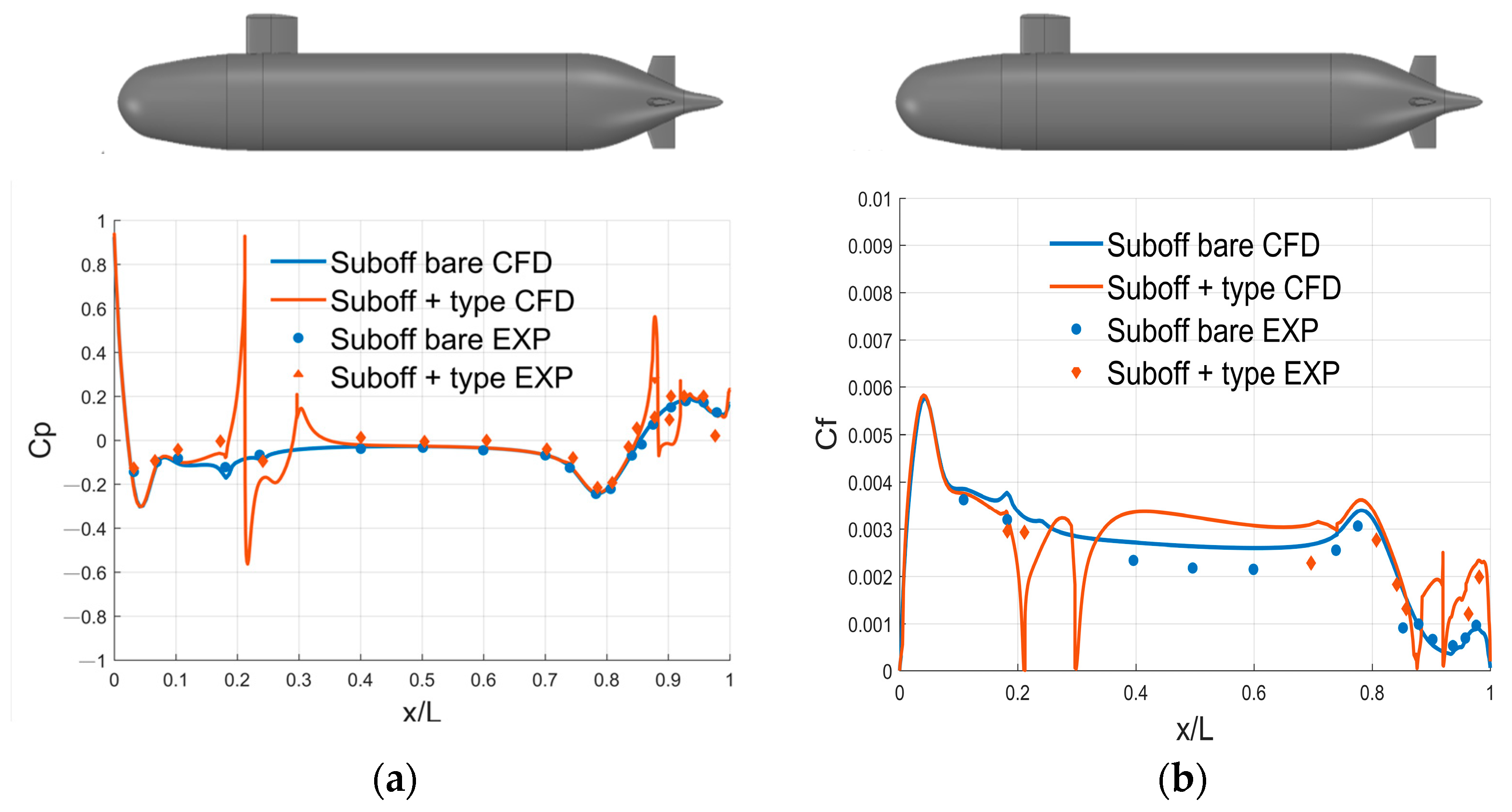
4.3. Analysis and Verification of Hull Resistance

In this study, the experimental boundary conditions were set as follows: The number of meshes in the computational domain was set to 6.77 million. Considering the verification of the submarine’s underwater characteristics’ calculation using the SST k-ω turbulence model, the results will be compared with the large eddy simulation [34] and experimental results [33]. The pressure coefficient $C_p$ and the Fanning friction factor $C_f$ are defined as

$$C_p=\frac{p}{0.5\rho U_{\infty }^2},$$

(20)

$$C_f=\frac{\tau }{0.5\rho U_{\infty }^2},$$

(21)

where p is the dynamic pressure.

For different ship speeds, the resistance of the hull with appendages is presented in

Table 6. Arrangement of thrust and torque coefficients for propellers installed on underwater vehicles at different speed.

${\mathit{U}}_{\mathit{\infty }}^{}$ (m/s)	[5] EXP. (N)	[34] LES (N) Diff. (%)	Present (N) Diff. (%)
3.050	102.3	106.4 (3.963%)	105.778 (3.40%)
6.096	389.2	384.6 (−1.173%)	384.566 (−1.19%)
7.161	526.6	519.2 (−1.408%)	519.682 (−1.31%)
9.152	821.1	820.5 (−0.067%)	822.645 (0.19%)

. The maximum deviation of the present procedure is 3.4%. Comparison of the numerical and experimental results [5] of the pressure coefficient and Fanning friction factor was carried out. As shown by the results, the calculated values exhibit the same trends as the experimental values. From Equation (20) to (21), the maximum oscillation of $C_p$ and $C_f$ occurs at discontinuous locations, such as the sail and four fins.

In this paper, we compared the pressure and friction coefficients around the hull to ensure that the calculated flow field used in this study is consistent with the actual flow field. After using the SST k-ω turbulence model to simulate and calculate, we carried out a comparison with results from the literature [5], as shown in Figure 18. The pressure curve rises sharply at the leading edge of the bow, sail cover, and stern rudder, and then falls. This is because the velocity of the fluid in the inflow direction changes at the mentioned position, resulting in a stagnation point at which the instantaneous velocity is zero. According to Bernoulli’s law, the total energy of a system should remain constant, and high pressure is generated when the flow velocity is slow. This results in a pressure coefficient $C_p$ ≈ 1 at the corresponding position. In the other flow field, the flow velocity is relatively fast, creating a velocity difference that leads to negative pressure at that position. The pressure coefficient may be presented as $C_p$ < 0. This occurs within the range of x/L 0.3~0.7 due to the hull wall being parallel to the inflow direction; thus, the speed change in this area is smaller than that in other areas. The flow velocity tends to be uniform for the inflow, and its pressure coefficient tends to zero. The Fanning friction coefficient ($C_f$) also follows the same trend. At the bow, sail cover, and stern rudder, there is a stagnation point. Therefore, there is no shear stress at these positions. The friction coefficient is presented as $C_f$ ≈ 0. After the stagnation point, the flow velocity in this area increases, resulting in a significant change in flow velocity and an increase in the friction coefficient.

4.4. Simulation Verification of Underwater Vehicle Self-Propulsion Test

In order to find the model-scale underwater sound field radiated noise, the experimental boundary conditions were set as follows: The number of meshes in the computational domain was set to 9.9 million, the fluid inflow velocity was set to $U_{\infty }^{}$= 9 m/s, and the propeller speed was set to 30.582 rps. The time it took for the propeller to rotate 1 degree was measured as a time step. A time interval Δt = 9.08305 × 10⁻⁵ s was used to estimate the first-order blade frequency of 214.074 Hz based on the basic theory of the propeller. The receiving field point was set at a distance of 1 m directly below the propeller, as referenced in the literature [8].

Table 7. Arrangement of thrust and torque coefficients for propellers installed on underwater vehicles.

Self-Propulsion
	[8] EXP. (N)	CFD (N)	Diff. (%)
KT	0.2618	0.2446	−6.57%
10KQ	0.4603	0.4651	1.02%

displays the coefficients of propeller thrust and torque derived from calculations in the self-propulsion test.

The propeller blade surface pressure calculated from the literature [8] shows consistent results, as shown in Figure 19. It can be observed that the trends of the two are consistent. Afterwards, we calculated the acoustic pressure of the self-propulsion test using both the FVM and BEM. We then compared the acoustic pressures obtained using the time-domain method in the literature [8] and the results obtained in this study, as shown in

Table 8. Noise acoustic pressure of the self-propulsion test.

BPF	[8] EXP SPL (dB)	CFD SPL (dB) Diff. (%)	BEM SPL (dB) Diff. (%)
1st BPF 214.06 Hz	116.8	111.98 (−4.13%)	111.6 (−4.45%)

. Upon comparison, we observed that FVM and the BEM have numerical errors of 4.13% and 4.45%, respectively, while maintaining the same level of numerical accuracy.

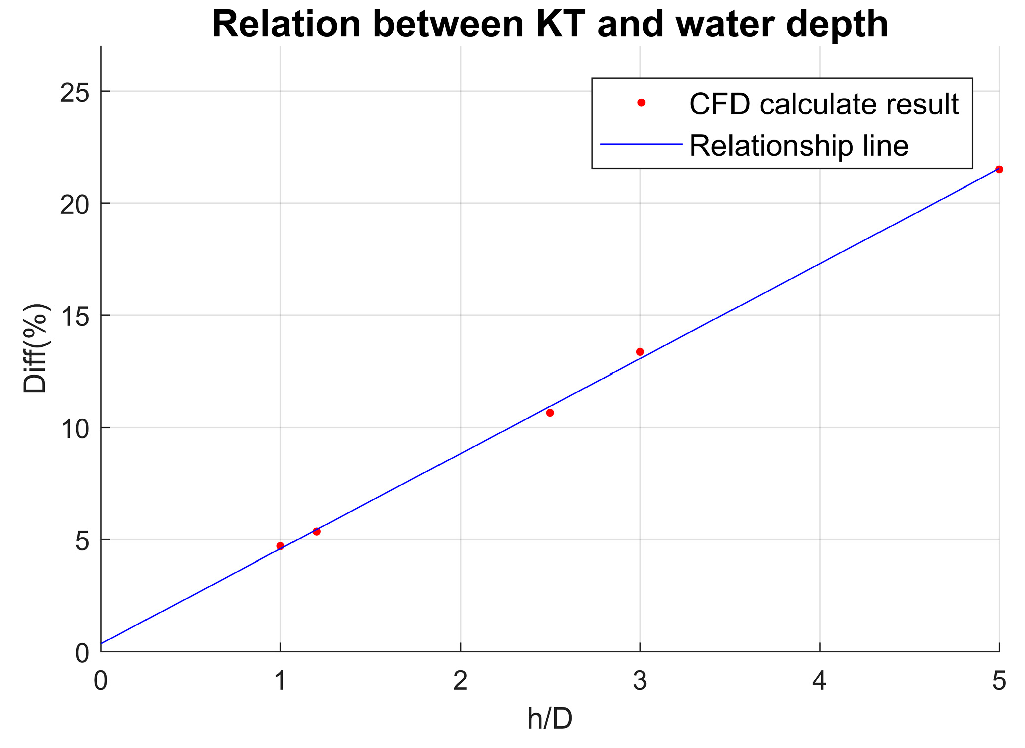
4.5. Propeller Performance Analysis of the Free Surface Effect

In this section, based on the experimental values of the open water test in [9], the VOF method was used to calculate the effect of the free surface plane on propeller performance. Through the thrust value of propeller, the relationship between water depth and pressure can be verified. The boundary conditions of the calculation domain are set as shown in Figure 20, with a total mesh count of 10.88 million. As shown in Figure 20, an area above the propeller was designated the free surface plane location (free surface). The fluid inlet was set as a velocity inflow (velocity inlet), and the outlet was set as an outlet (outlet). In the area surrounding the calculation domain, the symmetric boundary condition was adopted (symmetry).

As the literature [15] points out, the propeller is simultaneously affected depth and inflow velocity. Therefore, in this study, the advance ratio was fixed at 0.85 J, and the influence of the distance between the static water and the center of the propeller shaft center on its thrust torque was investigated. The propeller was placed at 1D, 1.2D, 2.5D, 3D, and 5D below the free surface, and the corresponding thrust coefficients were obtained, as shown in

Table 9. Water depth test position points and propeller thrust deviation.

h/D	h (m)	T (N)	KT EXP = 0.196
1	0.485	188.19	0.2052 4.7%
1.2	0.582	189.34	0.2069 5.34%
2.5	1.2125	198.88	0.2169 10.65%
3	1.455	203.76	0.2222 13.36%
5	2.425	218.37	0.2381 21.49%

. Comparing the simulation results with the literature [9], it can be observed that propeller thrust can reach the same level of thrust as in the experiment conducted in a cavitation tank at a specific water depth. Using the thrust coefficient from the literature [9] as the baseline, it can be observed from Figure 21 that as the water depth increases, the deviation between the thrust coefficient and the experimental values also increases. Since this result is consistent with the trends observed in the literature [13,14], it is reasonable to infer the water pressure of the propeller during the open water testing using Bernoulli’s law.

Finally, based on the experimental values of the self-propulsion test in [8], the VOF method was used to calculate the impact of the free surface plane on the performance of the underwater vehicle at a model scale. The boundary conditions of the calculation domain are set as shown in Figure 22, with a total mesh count of 9.9 million. In Figure 22, an area above the propeller was designated as the location of the free surface plane (free surface). The fluid inlet was set as a velocity inflow (velocity inlet), and the outlet was set as an outlet (outlet). The area surrounding the calculation domain adopts the symmetric boundary condition (symmetry).

Subsequently, the case of an underwater vehicle equipped with propellers was studied, and the underwater vehicles and propellers were placed at depths of 5D and 9D below the free surface. The thrust coefficients obtained through calculation and simulation are shown in

Table 10. Water depth test and thrust of the propeller mounted on the underwater vehicle.

h/Ds	h (m)	T (N)	KT EXP = 0.2618
5	1.31	1055.61	0.2400 −8.33%
9	2.358	1075.49	0.2445 −6.61%

. It can be seen that the thrust results of the same order can correspond to the experimental pressure found in the literature [8] at a water depth of 9D. Therefore, it can also be inferred that the water depth is equivalent to the water pressure in the water tank, as demonstrated in an experiment conducted in the literature [8]. In this study, the k-ω turbulence model was used to simulate the performance of the INSEAN E1619 seven-bladed propeller under various advance ratio conditions. The simulation results of propeller thrust, torque coefficient, and propulsion efficiency in this paper are consistent with the experimental values. This indicates that the research findings presented in this paper are applicable for engineering purposes.

5. Conclusions

In this study, in order to study the acoustic field radiation of an underwater vehicle under the free surface, the SST k-ω turbulence model was used to simulate and verify the propeller performance of the INSEAN E1619 seven-blade propeller under different propulsion ratios. The acoustic field radiation was calculated and experimental verification performed under different propulsion ratios using the DARPA SUBOFF model. For the underwater radiation simulation, a numerical procedure was combined with both the FVM and BEM to calculate the acoustic pressure of each field point measured at different distances. The FVM combines the fine mesh of the near field to achieve an accurate solution, while the BEM automatically satisfies the fundamental solution of the far field and obtains an accurate global sound field solution. The results of the self-propulsion test of the simulated underwater vehicle are consistent with the acoustic pressure levels obtained during the experiment. Finally, the numerical simulation calculations using the propeller under the free surface demonstrate that, at a specific water pressure, the propeller’s thrust can achieve results similar to experimental values. In addition, propeller thrust increases linearly with water depth. Moreover, the most important contributions of this study are the analysis of the noise directionality of the uniform inflow on the lower propeller and the utilization of a 3D model to visualize the direction of acoustic propagation at different frequencies. According to the relationship between water pressure and propeller thrust, it is possible to estimate propeller thrust at various water depths. Hence, the calculation results of this paper are consistent with experimental values, indicating that our research findings may have practical engineering applications. In future work, the present procedure will be applied to the study of full-scale underwater vehicles and verify the relationship between measurement range and hull length, at the same time, compared with the full scale of previous references [35]. In addition, this work can be extended to include sound source identification in order to analyze the scattering and radiation issues that occur between an underwater vehicle and the free surface.

References

1. Song, K.W.; Guo, C.Y.; Wang, C.; Sun, C.; Li, P.; Wang, W. Numerical analysis of the effects of stern flaps on ship resistance and propulsion performance. Ocean Eng. 2019, 193, 106621. [Google Scholar] [CrossRef]
2. Moura, N.D.; Seixas, J.; Ramos, R. Passive sonar signal detection and classification based on independent component analysis. In Sonar Systems; InTech: Makati, Philippines, 2011. [Google Scholar]
3. Wittekind, D.; Schuster, M. Propeller cavitation noise and background noise in the sea. Ocean Eng. 2016, 120, 116–121. [Google Scholar] [CrossRef]
4. Groves, N.C.; Huang, T.T.; Chang, M.S. Geometric Characteristics of DARPA (Defense Advanced Research Projects Agency) SUBOFF Models (DTRC Model Numbers 5470 and 5471); David W Taylor Naval Ship Research and Development Center: Carderock, MD, USA, 1989. [Google Scholar]
5. Liu, H.L.; Huang, T.T. Summary of DARPA Suboff Experimental Program Data; Naval Surface Warfare Center, Carderock Division (NSWCCD): Carderock, MD, USA, 1998. [Google Scholar]
6. Menter, F.R. Two-equation eddy-viscosity turbulence models for engineering applications. AIAA J. 1994, 32, 1598–1605. [Google Scholar]
7. Chase, N. Simulations of the DARPA Suboff Submarine including Self-Propulsion with the E1619 Propeller. Master’s Thesis, University of Iowa, Iowa, IA, USA, 2012. [Google Scholar]
8. Choi, J.H. Numerical Analysis on Underwater Propeller Noise with Hull-Appendage Effect. Master’s Thesis, Seoul National University, Seoul, Republic of Korea, 2019. [Google Scholar]
9. Felice, F.D.; Felli, F.M.; Liefvendahl, M.; Svennberg, U. Numerical and experimental analysis of the wake behavior of a generic submarine propeller. In Proceedings of the First International Symposium on Marine Propulsors, Trondheim, Norway, 22–24 June 2009. [Google Scholar]
10. Hirt, C.W.; Nichols, B.D. Volume of fluid (VOF) method for the dynamics of free boundaries. J. Comp. Phys. 1981, 39, 201–225. [Google Scholar] [CrossRef]
11. Califano, A.; Steen, S. Numerical simulations of a fully submerged propeller subject to ventilation. Ocean Eng. 2011, 38, 1582–1599. [Google Scholar] [CrossRef]
12. Paik, K.J. Numerical study on the hydrodynamic characteristics of a propeller operating beneath a free surface. Int. J. Nav. Archit. Ocean Eng. 2017, 9, 655–667. [Google Scholar] [CrossRef]
13. Eom, M.J.; Jang, Y.H.; Paik, K.J. A study on the propeller open water performance due to immersion depth and regular wave. Ocean Eng. 2021, 219, 108265. [Google Scholar] [CrossRef]
14. Eom, M.J.; Paik, K.J.; Jang, Y.H.; Ha, J.Y.; Park, D.W. A method for predicting propeller performance considering ship motion in regular waves. Ocean Eng. 2021, 232, 109135. [Google Scholar] [CrossRef]
15. Cianferra, M.; Armenio, V. Scaling properties of the Ffowcs-Williams and Hawkings equation for complex acoustic source close to a free surface. J. Fluid Mech. 2021, 927, A2. [Google Scholar] [CrossRef]
16. Hu, J.; Ning, X.S.; Zhao, W.; Li, F.G.; Ma, J.C.; Zhang, W.P.; Sun, S.L.; Zou, M.S.; Lin, C.G. Numerical simulation of the capitating noise of contra-rotating propellers based on detached eddy simulation and the Ffowcs Williams–Hawkings acoustics equation. Phys. Fluids 2021, 33, 116–121. [Google Scholar] [CrossRef]
17. Noughabi, A.K.; Bayati, M.; Tadjfar, M. Investigation of cavitation phenomena on noise of underwater Propeller. In Proceedings of the ASME 2017 Fluids Engineering Division Summer Meeting, Waikoloa, HI, USA, 30 July–3 August 2017; pp. 1–8. [Google Scholar]
18. TM-2007-214853; Farassat, F. Derivation of Formulations 1 and 1A of Farassat. NASA: Washington, DC, USA, 2007.
19. Koushan, K.; Spence, S.J.; Hamstad, T. Experimental investigation of the effect of waves and ventilation on thruster loadings. In Proceedings of the 1st International Symposium on Marine Propulsors, Trondheim, Norway, 22–24 June 2009. [Google Scholar]
20. Paik, B.G.; Lee, C.M.; Lee, S.J. Comparative measurements on the flow structure of a marine propeller wake between an open free surface and closed surface flows. J. Mar. Sci. Technol. 2005, 10, 123–130. [Google Scholar] [CrossRef]
21. Kim, S.; Kinnas, S.A. Prediction of acoustic field induced by a tidal turbine under straight or oblique inflow via a BEM/FW-H approach. Ocean Syst. Eng. 2023, 13, 147–172. [Google Scholar]
22. Yao, Q.; Zhang, Y.O.; Li, Y.F.; Zhang, T. Similarity analysis of the flow-induced noise of a benchmark submarine. Front. Phys. 2023, 11, 270. [Google Scholar]
23. Kimmerl, J.; Moustafa, A.M. Visualization of underwater radiated noise in the near-and far-field of a propeller-hull configuration using CFD simulation results. J. Mar. Sci. Eng. 2023, 11, 834. [Google Scholar] [CrossRef]
24. Wilcox, D.C. Turbulence Modeling for CFD; DCW Industries: La Cañada, CA, USA, 1998. [Google Scholar]
25. Launder, B.E.; Spalding, D.B. Lectures in Mathematical Models of Turbulence; Academic Press: London, UK, 1972. [Google Scholar]
26. Menter, F.; Ferreira, J.C.; Esch, T.; Konno, B. The SST turbulence model with improved wall treatment for heat transfer predictions in gas turbines. In Proceedings of the International Gas Turbine Congress, Tokyo, Japan, 2–7 November 2003. [Google Scholar]
27. Menter, F.R. Review of the shear-stress transport turbulence model experience from an industrial perspective. Int. J. Comput. Fluid Dyn. 2009, 23, 305–316. [Google Scholar] [CrossRef]
28. Lighthill, M.J. On sound generated aerodynamically I. General theory. Philos. Trans. Ser. A Math. Phys. Sci. 1952, 211, 564–587. [Google Scholar]
29. Lighthill, M.J. On sound generated aerodynamically II. Turbulence as a source of sound. Philos. Trans. Ser. A Math. Phys. Sci. 1954, 212, 1–32. [Google Scholar]
30. Williams, J.F.; Hawkings, D.L. Sound generation by turbulence and surfaces in arbitrary motion. Philos. Trans. Ser. A Math. Phys. Sci. 1969, 264, 321–342. [Google Scholar]
31. Desmet, W.; Sas, P.; Vandepitte, D. Numerical Acoustics Theoretical Manual; LMS International: Leuven, Belgium, 1998. [Google Scholar]
32. Geng, F.; Kalkman, I.; Suiker, A.S.J.; Blocken, B. Sensitivity analysis of airfoil aerodynamics during pitching motion at a Reynolds number of 1.35 × 10⁵. J. Wind Eng. Ind. Aerodyn. 2018, 183, 315–332. [Google Scholar]
33. Guo, H.; Guo, C.Y.; Hu, J.; Lin, J.F.; Zhong, X.H. Influence of jet flow on the hydrodynamic and noise performance of propeller. Phys. Fluids 2021, 33, 065123. [Google Scholar]
34. Chiu, S.J. Hull Shape Optimization Design and Hydrodynamics Analysis of an Underwater Vehicle. Master’s Thesis, National Taiwan Ocean University, Taiwan, China, 2018. [Google Scholar]
35. Liu, L.W.; Chen, M.X.; Yu, J.W.; Zhang, Z.G. Full-scale simulation of self-propulsion for a free-running submarine. Phys. Fluids 2021, 33, 047103. [Google Scholar]
Figure 1. Schematic diagram of the E1619 propeller model.
Jmse 11 01940 g001
Figure 2. Computational domain geometry setup.
Jmse 11 01940 g002
Figure 3. Boundary condition settings.
Jmse 11 01940 g003
Figure 4. Computational meshes of calculation domain: (a) mesh of the static and rotating subdomains, and (b) refinements near the propeller surface.
Jmse 11 01940 g004
Figure 5. Comparison of experimental and simulation values of thrust coefficient, torque coefficient, and propulsion efficiency.
Jmse 11 01940 g005
Figure 6. Propeller pressure distribution: (a) thrust surface; (b) resistance surface.
Jmse 11 01940 g006
Figure 7. Schematic diagram of each field point in the radial and axial directions.
Jmse 11 01940 g007
Figure 8. Pressure pulsations at each field point in the radial direction: (a) 1D; (b) 2.5D; (c) 5D; and (d) 10D.
Jmse 11 01940 g008aJmse 11 01940 g008b
Figure 9. Pressure pulsations in the axial direction at each field point: (a) 1D; (b) 2.5D; (c) 5D; and (d) 10D.
Jmse 11 01940 g009
Figure 10. Absolute value of pressure at each field point in the radial direction at a time of 1.6 s.
Jmse 11 01940 g010
Figure 11. The absolute value of the pressure at each field point in the axis direction at a time of 1.6 s.
Jmse 11 01940 g011
Figure 12. Comparison of acoustic pressure spectrum at radial field points: (a) 1D; (b) 2.5D; (c) 5D; and (d) 10D.
Jmse 11 01940 g012
Figure 13. Comparison of acoustic pressure spectra at axial field points: (a) 1D; (b) 2.5D; (c) 5D; and (d) 10D.
Jmse 11 01940 g013
Figure 14. Three-dimensional model of energy transfer direction at each frequency: (a) 4.0752 Hz, (b) 8.1504 Hz, (c) 12.2256 Hz, (d) 16.3008 Hz, (e) 20.376 Hz, (f) 24.4512 Hz, (g) 28.5264 Hz, and (h) schematic diagram of the propeller rotation axis.
Jmse 11 01940 g014
Figure 15. The DARPA SUBOFF model geometry schematic (AFF8+).
Jmse 11 01940 g015
Figure 16. Computational domain: (a) geometry parameters and (b) boundary conditions.
Jmse 11 01940 g016
Figure 17. Hull diagram of a cross rudder with full appendages.
Jmse 11 01940 g017
Figure 18. Comparison of numerical and experimental results [5]: (a) pressure coefficient and (b) Fanning friction factor.
Jmse 11 01940 g018
Figure 19. Surface pressure diagram of the propeller blade during the self-propulsion test.
Jmse 11 01940 g019
Figure 20. Propeller-only computational domain: (a) boundary conditions and (b) meshes of the calculation domain.
Jmse 11 01940 g020
Figure 21. A linear relationship between water depth and propeller thrust deviation.
Jmse 11 01940 g021
Figure 22. Submarine hull only computational domain: (a) boundary conditions and (b) meshes of the calculation domain.
Jmse 11 01940 g022