
Assessment of Wave Power Density Using Sea State Climate Change Initiative Database in the French Façade


Abstract
:1. Introduction
2. Material and Methods
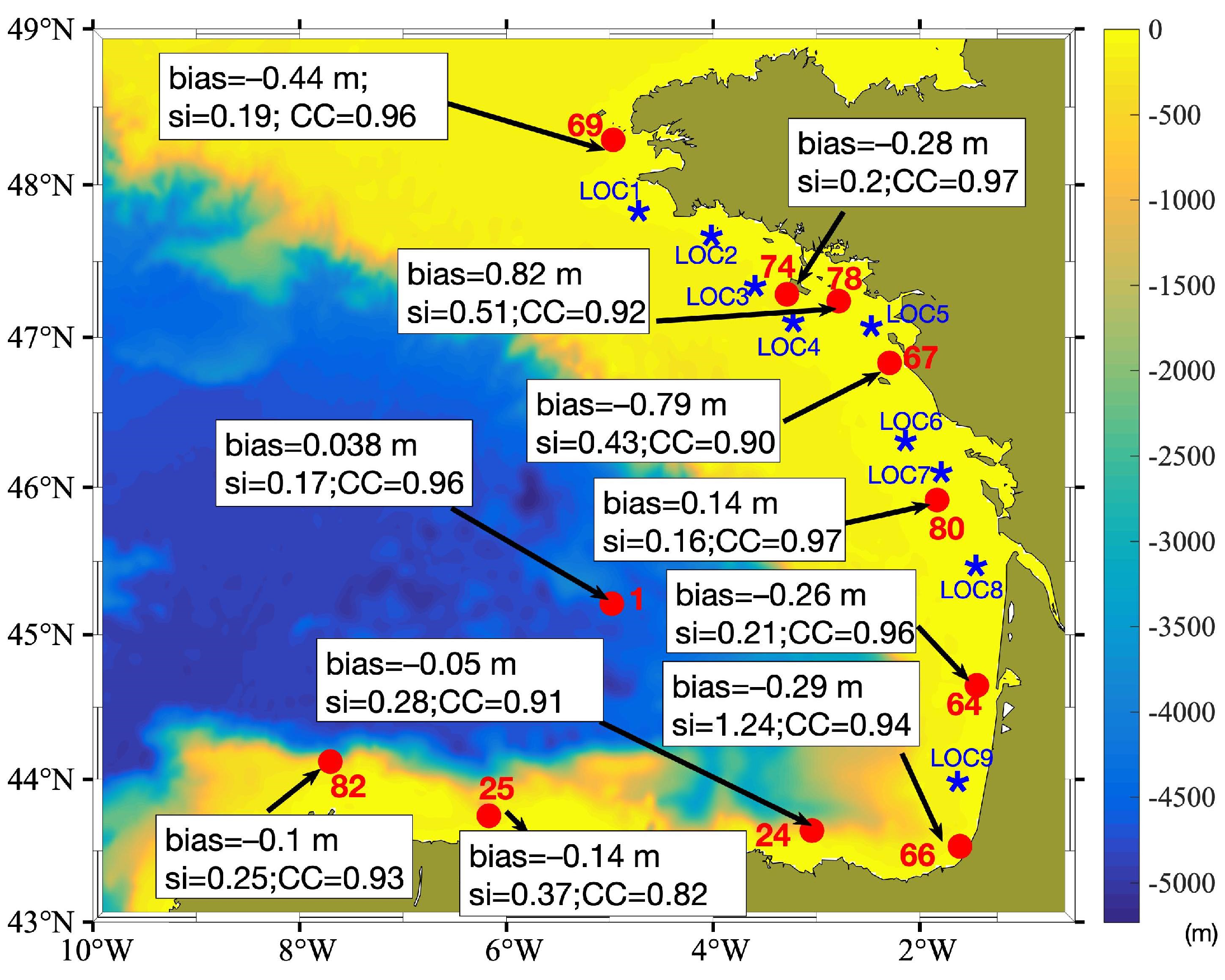
2.1. The French Façade
2.2. Data
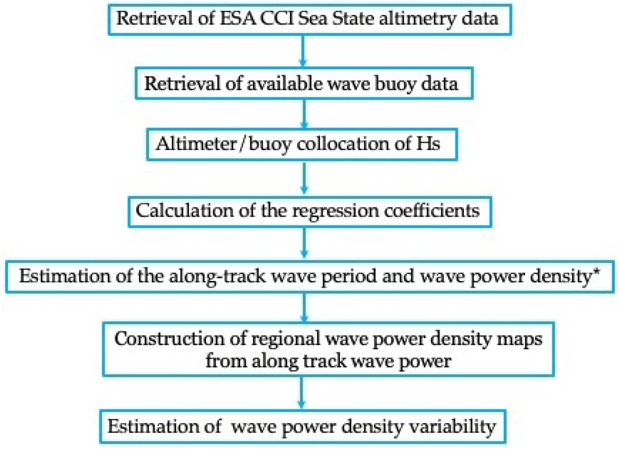
2.3. The Wave Power Estimation Method
2.3.1. Wave Power Density
2.3.2. Empirical Estimation of Tz
2.3.3. Coefficients of Variability
3. Results and Discussion
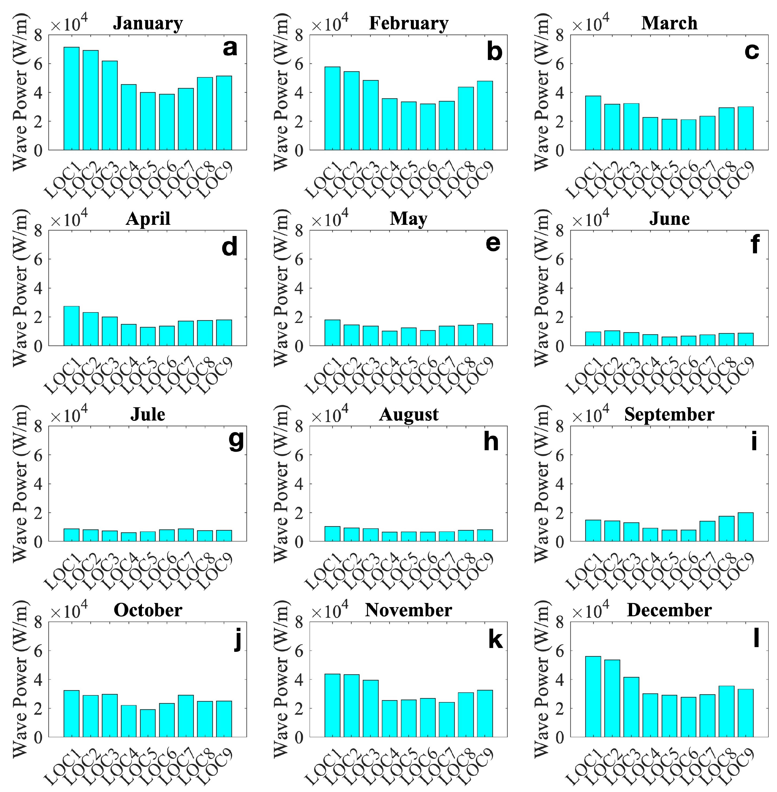
Seasonal Analysis
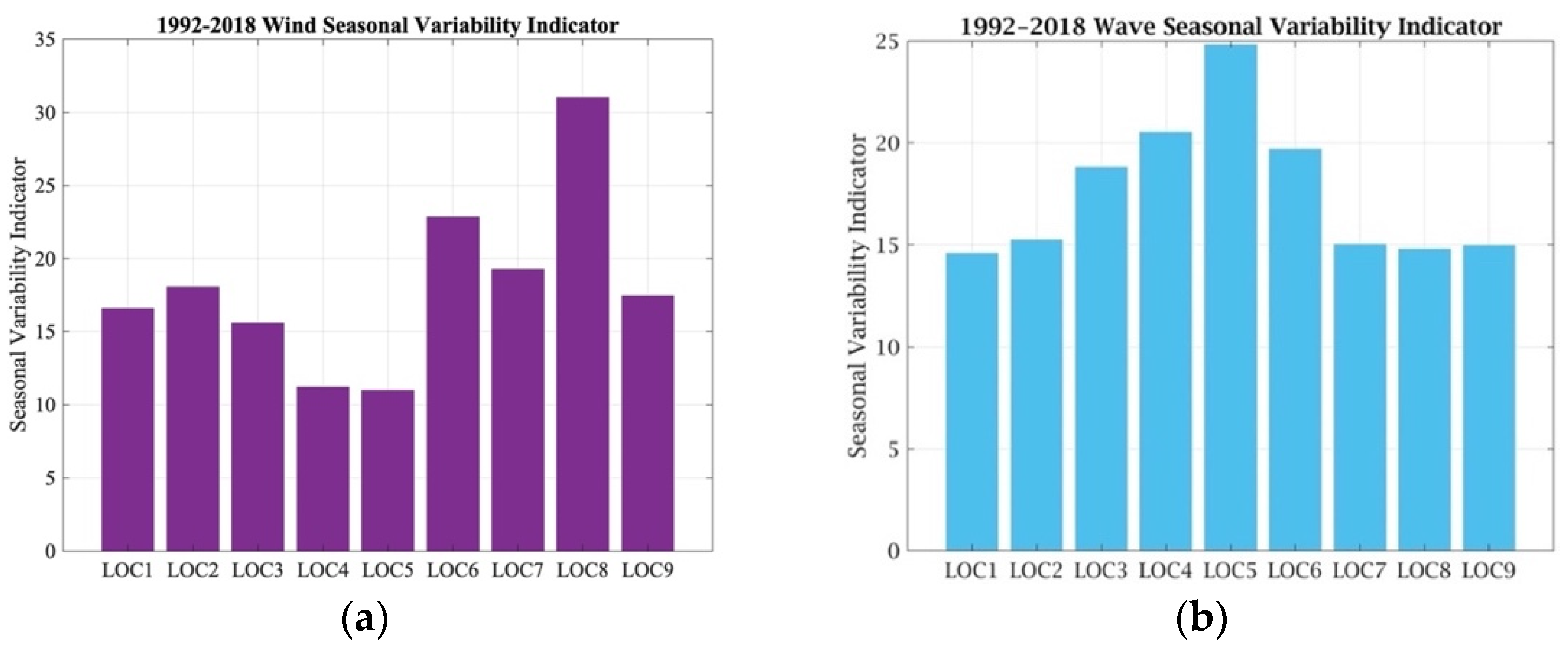
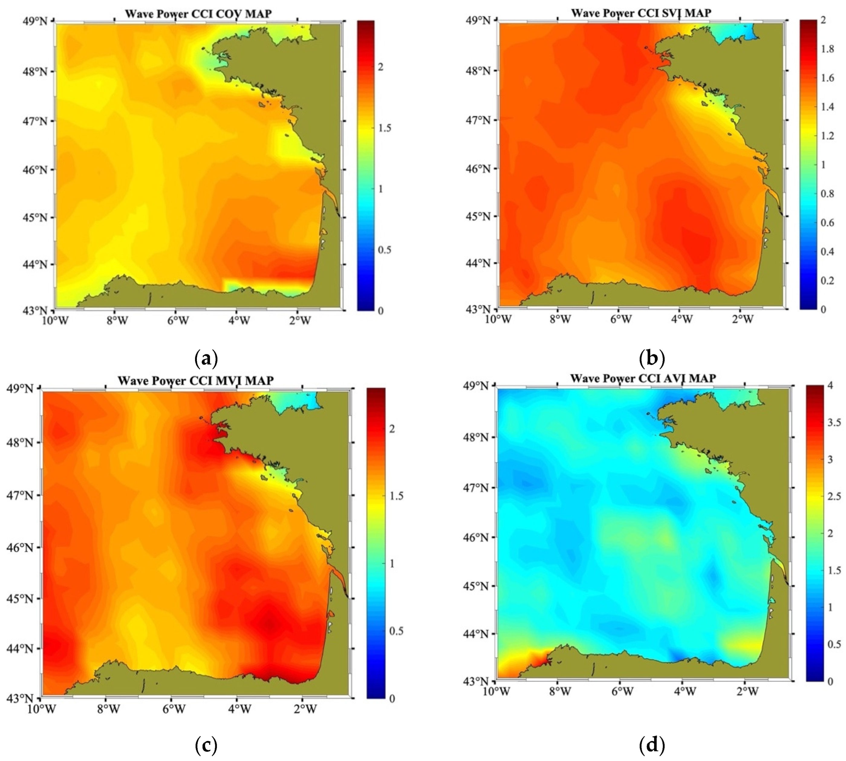
4. Variability
5. Conclusions
Author Contributions
Funding
Data Availability Statement
Acknowledgments
Conflicts of Interest
References
- Peña-Sanchez, Y.; García-Violini, D.; Ringwood, J.V. Control co-design of power take-off parameters for wave energy systems. IFAC-Pap. 2022, 55, 311–316. [Google Scholar] [CrossRef]
- Guillou, N.; Lavidas, G.; Chapalain, G. Wave Energy Resource Assessment for Exploitation—A Review. J. Mar. Sci. Eng. 2020, 8, 705. [Google Scholar] [CrossRef]
- Henderson, R. Design, simulation, and testing of a novel hydraulic power take-off system for the Pelamis wave energy converter. Renew. Energy 2006, 31, 271–283. [Google Scholar] [CrossRef]
- Eco Wave Power. Available online: https://www.ecowavepower.com/future-projects/ (accessed on 7 September 2020).
- Reguero, B.; Losada, I.J.; Mendez, J.F. A recent increase in global wave power as a consequence of oceanic warming. Nat. Commun. 2019, 10, 205. [Google Scholar] [CrossRef] [PubMed]
- Amarouche, K.; Akpınar, A.; El Islam Bachari, N.; Houma, F. Wave energy resource assessment along the Algerian coast based on 39-year wave hindcast. Renew. Energy 2020, 153, 840–860. [Google Scholar] [CrossRef]
- Silva, D.; Rusu, E.; Guedes Soares, C. Evaluation of the expected power output of wave energy converters in the north of the Portuguese nearshore. In Progress in Renewable Energies Offshore; Guedes Soares, C., Ed.; Taylor & Francis Group: London, UK, 2016; pp. 875–882. [Google Scholar]
- Silva, D.; Martinho, P.; Guedes Soares, C. Wave energy distribution along the Portuguese continental coast based on a thirty three years hindcast. Renew. Energy 2018, 127, 1064–1075. [Google Scholar] [CrossRef]
- Ponce de León, S.; Orfila, A.; Simarro, G. Wave energy in the Balearic Sea. Evolution from a 29 years spectral wave hindcast. Renew. Energy 2016, 82, 1192–1200. [Google Scholar] [CrossRef]
- Rusu, L.; Rusu, E. Evaluation of the Worldwide Wave Energy Distribution Based on ERA5 Data and Altimeter Measurements. Energies 2021, 14, 394. [Google Scholar] [CrossRef]
- Guillou, N.; Chapalain, G. Numerical Modelling of Nearshore Wave Energy Resource in the Sea of Iroise. Renew. Energy 2015, 83, 942–953. [Google Scholar] [CrossRef]
- Guillou, N.; Lavidas, G.; Kamranzad, B. Wave Energy in Brittany (France)—Resource Assessment and WEC Performances. Sustainability 2023, 15, 1725. [Google Scholar] [CrossRef]
- Guillou, N.; Neill, S.P.; Thiébot, J. Spatio-Temporal Variability of Tidal-Stream Energy in North-Western Europe. Phil. Trans. R. Soc. A 2020, 378, 20190493. [Google Scholar] [CrossRef] [PubMed]
- Goncalves, M.; Martinho, P.; Guedes Soares, C. A 33-year hindcast on wave energy assessment in the western French coast. Energy 2018, 165, 790–801. [Google Scholar] [CrossRef]
- Dodet, G.; Piolle, J.-F.; Quilfen, Y.; Abdalla, S.; Accensi, M.; Ardhuin, F.; Ash, E.; Bidlot, J.-R.; Gommenginger, C.; Marechal, G.; et al. The Sea State CCI dataset v1: Towards a sea state climate data record based on satellite observations. Earth Syst. Sci. Data 2020, 12, 1929–1951. [Google Scholar] [CrossRef]
- Ponce de León, S.; Restano Benveniste, J.M. Assessment of wave power in the French façade inferred from high-resolution altimetry. Remote Sens. 2023. in preparation. [Google Scholar]
- Ponce de León, S.; Bettencourt, J.; Ringwood, J.V.; Benveniste, J. Assessment of combined wind and wave energy in European coastal waters using satellite altimetry. Appl. Ocean. Res. 2023. under review. [Google Scholar]
- Rusu, E.; Rusu, L. An evaluation of the wave energy resources in the proximity of the wind farms operating in the North Sea, 438. Energy Rep. 2021, 7, 19–27. [Google Scholar] [CrossRef]
- Idris, N.H. Wave energy resource assessment with improved satellite altimetry data over the Malaysian coastal sea. Arab. J. Geosci. 2019, 12, 484. [Google Scholar] [CrossRef]
- Uti, M.N.; Din, A.H.M.; Yaakob, O. Significant wave height assessment using multi mission satellite altimeter over Malaysian seas. IOP Conf. Ser. Earth Environ. Sci. 2018, 169, 012025. [Google Scholar] [CrossRef]
- Dinardo, S. Techniques and Applications for Satellite SAR Altimetry over Water, Land and Ice. Ph.D. Thesis, Technische Universität, Darmstadt, Germany, 2020. Volume 56, ISBN 978-3-935631-45-7. [Google Scholar] [CrossRef]
- Dinardo, S.; Fenoglio-Marc, L.; Buchhaupt, C.; Becker, M.; Scharroo, R.; Fernandes, M.J.; Benveniste, J. Coastal SAR and PLRM altimetry in German Bight and West Baltic sea. Adv. Space Res. 2018, 62, 1371–1404. [Google Scholar] [CrossRef]
- Gommenginger, C.P.; Srokosz, M.A.; Challenor, P.G.; Cotton, P.D. Measuring ocean wave period with satellite altimeters: A simple empirical model. Geophys. Res. Lett. 2003, 30, 2150. [Google Scholar] [CrossRef]
- Abdalla, S.; Kolahchi, A.A.; Ablain, M.; Adusumilli, S.; Bhowmick, S.A.; Alou-Font, E.; Amarouche, L.; Andersen, O.B.; Antich, H.; Aouf, L.; et al. Altimetry for the future: Building on 25 years of progress. Adv. Space Res. 2021, 68, 319–363. [Google Scholar] [CrossRef]
- Ringwood, J.V.; Brandle, G. A new world map for wave power with a focus on variability. In Proceedings of the 11th European Wave and Tidal Energy Conference, Nantes, France, 6–11 September 2015; Available online: https://mural.maynoothuniversity.ie/6682/1/JR_new%20world%20map.pdf (accessed on 16 December 2022).
- Cahill, B.; Lewis, T. Wave Periods and the Calculation of Wave Power; Virginia Tech: Blacksburg, VA, USA, 2014; p. 46259438. [Google Scholar]
- Hasselmann, K.; Barnett, T.P.; Bouws, E.; Carlson, H.; Cartwright, D.E.; Enke, K.; Ewing, J.A.; Gienapp, A.; Hasselmann, D.E.; Kruseman, P.; et al. Measurements of Wind-Wave Growth and Swell Decay during the Joint North Sea Wave Project (JONSWAP); Deutsches Hydrographisches Institut: Hamburg, Germany, 1973. [Google Scholar]
- Amiruddin; Ribal, A.; Khaeruddin; Thamrin, S.A. A 10-year wave energy resource assessment and trends of Indonesia based on satellite 436 observations. Acta Oceanol. Sin. 2019, 38, 86–93. [Google Scholar] [CrossRef]
- Schlembach, F.; Ehlers, F.; Kleinherenbrink, M.; Passaro, M.; Dettmering, D.; Seitz, F.; Slobbe, C. Benefits of fully focused SAR altimetry to coastal wave height estimates: A case study in the North Sea. Remote Sens. Environ. 2023, 289, 113517. [Google Scholar] [CrossRef]
- Fusco, F.; Nolan, G.; Ringwood, J. Variability reduction through optimal combination of wind/waves resources—An Irish case study. Energy 2010, 35, 310–325. [Google Scholar] [CrossRef]
- Sierra, J.P.; White, A.; Mosso, C.; Mestres, M. Assessment of the intra-annual and inter-annual variability of the wave energy resource in the Bay of Biscay (France). Energy 2017, 141, 853–868. [Google Scholar] [CrossRef]


| Buoys | Regression Coefficients |
|---|---|
| 78 (2010–2018) | a = 1.4302; b = 1.6812 |
| 67 (2005–2018) | a = 1.1129; b = 2.672 |
| 69 (2008–2018) | a = 1.5917; b = 2.0901 |
| 64 (2004–2018) | a = 1.713; b = 2.0250 |
| 74 (2011–2018) | a = 1.6616; b = 1.7943 |
| 80 (2014–2018) | a = 2.216; b = 0.571 |
| 66 (2004–2018) | a = 2.210; b = 1.3477 |
| 1 (1998–2018) | a = 1.8834; b = 1.8863 |
| 24 (1990–2018) | a = 1.9861; b = 1.1065 |
| 25 (1996–2018) | a = 1.7340; b = 1.649 |
| 82 (1997–2018) | a = 1.6790; b = 1.517 |
Disclaimer/Publisher’s Note: The statements, opinions and data contained in all publications are solely those of the individual author(s) and contributor(s) and not of MDPI and/or the editor(s). MDPI and/or the editor(s) disclaim responsibility for any injury to people or property resulting from any ideas, methods, instructions or products referred to in the content. |
© 2023 by the authors. Licensee MDPI, Basel, Switzerland. This article is an open access article distributed under the terms and conditions of the Creative Commons Attribution (CC BY) license (https://creativecommons.org/licenses/by/4.0/).
Share and Cite
Ponce de León, S.; Restano, M.; Benveniste, J. Assessment of Wave Power Density Using Sea State Climate Change Initiative Database in the French Façade. J. Mar. Sci. Eng. 2023, 11, 1970. https://doi.org/10.3390/jmse11101970
Ponce de León S, Restano M, Benveniste J. Assessment of Wave Power Density Using Sea State Climate Change Initiative Database in the French Façade. Journal of Marine Science and Engineering. 2023; 11(10):1970. https://doi.org/10.3390/jmse11101970
Chicago/Turabian StylePonce de León, Sonia, Marco Restano, and Jérôme Benveniste. 2023. "Assessment of Wave Power Density Using Sea State Climate Change Initiative Database in the French Façade" Journal of Marine Science and Engineering 11, no. 10: 1970. https://doi.org/10.3390/jmse11101970