Numerical Investigation on Interactive Hydrodynamic Performance of Two Adjacent Unmanned Underwater Vehicles (UUVs)

Abstract

This study investigates the effectiveness of UUV formations during navigation to designated target areas. The research focuses on propeller-equipped UUVs and employs a computational fluid dynamics (CFD) methodology to analyze the hydrodynamic interactions among multiple UUV formations while en route to their targeted exploration areas. Utilizing the relative drag coefficients ($r_l \mathrm{a}\mathrm{n}\mathrm{d} r_f$) and static thrust ($R_{fleets}$) as analytical parameters, this paper defines the relative distances ($a$ and $b$) between UUVs within a formation and conducts a comparative analysis of the hydrodynamic performance between individual UUVs and formation configurations. The study establishes correlations between relative distances and the hydrodynamic performance of formations. The findings reveal the following: 1. For both the lead UUV and the following UUV within the formation, the $r_l \mathrm{a}\mathrm{n}\mathrm{d} r_f$ heatmaps exhibit two distinct regions: a thrust region and a drag region. Notably, these regions significantly overlap. The maximum $r_l$ is 31.23%, while the minimum $r_f$ is −20.9%, corresponding to relative distances of $a$ = 0.12 and $b$ = 1.5. Conversely, the minimum $r_l$ is −12.2%, while the maximum $r_f$ is 22.03%, with relative distances of $a$ = 1.1 and $b$ = 0.2; 2. An analysis of formation static thrust $R_{fleets}$ reveals that it can be up to 7% greater than the drag experienced by self-propelled UUVs when relative distances $a$ and $b$ are set to 1.1 and 1, respectively. This highlights the enhanced performance achievable through formation navigation. The results presented in this paper offer valuable theoretical insights into the optimal design of relative distances within UUV formations, contributing to the advancement of UUV formation navigation strategies.

1. Introduction

Unmanned underwater vehicles (UUVs), as intricate multidisciplinary entities, encompass a fusion of technologies, including underwater communication, automatic control, pattern recognition, and artificial intelligence. They possess the capability to autonomously conduct underwater operations without human intervention [1]. Since their inception, UUVs have emerged as pivotal tools for ocean observation and have found extensive application in marine environment monitoring, submarine oil and gas pipeline inspection, cable detection, hydrological research, and various other domains. As UUV technology continues to advance and marine engineering requirements evolve, the concept of multi-UUV collaboration has gained prominence. The operational workflow of multi-UUVs, owing to their concealed nature, typically includes stages such as UUV deployment, formation assembly, task allocation and planning, communication and information sharing, state sensing and environment modeling, system control and path planning, collision avoidance and collaborative decision-making, task execution, and evaluation.

Due to their high operational efficiency, strong execution capabilities, and broad mission profiles, research into multi-UUV collaboration has garnered increased attention from the scientific and engineering communities. While existing research predominantly centers on formation control and cooperative navigation [2,3,4,5,6,7,8], limited attention has been devoted to the hydrodynamic performance of UUV formations during their journey to target areas.

The effectiveness of UUV formations can significantly influence energy efficiency and collision avoidance among UUVs. Evaluating the hydrodynamic performance of a formation entails considering not only an individual UUV’s hydrodynamics but also the impact of relative distances between UUVs during formation navigation. Key areas of focus in formation hydrodynamics encompass the resistance of individual UUVs and the predictive modeling of UUV speeds. Several studies have contributed to this understanding:

Jagadeesh et al. [9] conducted experimental investigations using a towing flume to determine axial, normal, drag, lift, and pitching moment coefficients of an AUV at various angles of attack. Guo et al. [10] introduced a CFD-based method to explore the correlation between vehicle attitude and drag variation in surface-navigating vehicles, substantiated through experimental validation. Vali et al. [11] investigated hull/propeller interactions in submerged and surface conditions for a submarine model with realistic geometry. Yang et al. [12] developed a numerical design method for long-range AUV propellers based on RANS calculations. Posa Antonio et al. [13] simulated the vortex field generated by a submarine stern propeller, highlighting the influence of loading conditions on hub vortices and blade tip vortices. Pablo M. Carrica et al. [14] conducted comparative CFD studies on UUV self-propulsion in calm water and in head-on waves, emphasizing the importance of considering the coupling between hull dynamics and ambient flow in wave conditions. J. Ezequiel Martin et al. [15] conducted an experimental and computational fluid dynamics study of a DARPA Suboff submarine equipped with a seven-bladed E1658 propeller, highlighting the influence of submarine presence and its interaction with the free surface on propeller inflow and wake. Luo et al. [16] explored the hydrodynamic performance of a UUV under different conditions, including near the free liquid surface, near ice, and at infinite depths, using CFD.

Research on the navigational stability and maneuverability of a self-propelled vehicle under the influence of ocean currents primarily centers on the investigation of attitude control in autonomous underwater helicopters (AUHs) [17]. SHI Kai et al. investigated the problem of model-free control in the initial direction of a disc-shaped autonomous underwater helicopter. They addressed the issue by utilizing a model-free adaptive sliding mode controller, which effectively merges model-free adaptive control with jitter-free sliding mode control [18]. Haoda Li and his colleagues employed a data-driven methodology to execute an LADRC-TD algorithm, which facilitated successful control over the non-overlapping water depth and heading [19]. Du Penzhou et al. developed an adaptive inverse stepping sliding mode control (ABSMC) algorithm for the lightweight autonomous underwater helicopter (AUH). The ABSMC algorithm effectively addresses the highly coupled nonlinearities, manages unknown system parameters, handles disturbance uncertainty, and mitigates input saturation [20].

However, research on the relative positions of UUVs within a formation has received limited attention. Molland et al. [21] examined the effects of ellipsoidal proximity, time viscous effects, and viscous interactions in flow fields, suggesting that numerical simulations hold promise for studying these effects. In contrast, Tian et al. [22] employed CFD and artificial intelligence techniques to predict drag performance relationships among formation UUVs based on relative distance, optimizing the relative distance to minimize drag.

In summary, existing literature primarily focuses on simplified UUV models without propellers when studying the relative positions of UUVs in formations. Such models overlook the mutual interference between propellers and bare UUVs, as well as interactions between propellers and neighboring UUVs. To address this gap and provide hydrodynamic coupling relations for the study of control algorithms among multiple unmanned underwater vehicles (UUVs), this paper examines UUVs equipped with propellers. Studying the impact of relative distances among UUVs in formations on their hydrodynamic performance holds significant importance. This study establishes a hydrodynamic model for a single UUV with a propeller $R_e=1\times {10}^6$ to determine propeller rotation speed, UUV drag, and propeller thrust in self-propelled conditions. Subsequently, the propeller rotation speed in a multi-UUV model is aligned with that of the single-UUV model to assess the hydrodynamic performance of the multi-UUV configuration under various spacing ratios. The analysis aims to elucidate the influence of spacing ratios on the multi-UUV formation’s hydrodynamic performance, utilizing the performance of the single UUV as a reference benchmark.

Section 2 describes the dimensions of the underwater vehicle model and defines the dimensionless parameters used to analyze numerical results. Section 3 provides a detailed explanation of the chosen numerical method, including boundary conditions and the mesh model, with a focus on validating its feasibility. In Section 4, the baseline hydrodynamic performance of a single vehicle is established through a self-propelled numerical test. The paper conducts a comparative analysis of the impact of vehicle formation positions on the hydrodynamic performance of leading and trailing vehicles. Section 5 presents the findings, while Nomenclature explains the parameters utilized in the study.

The flow chart of the research methodology and the contents of this paper are shown in Figure 1.

2. Materials and Methods

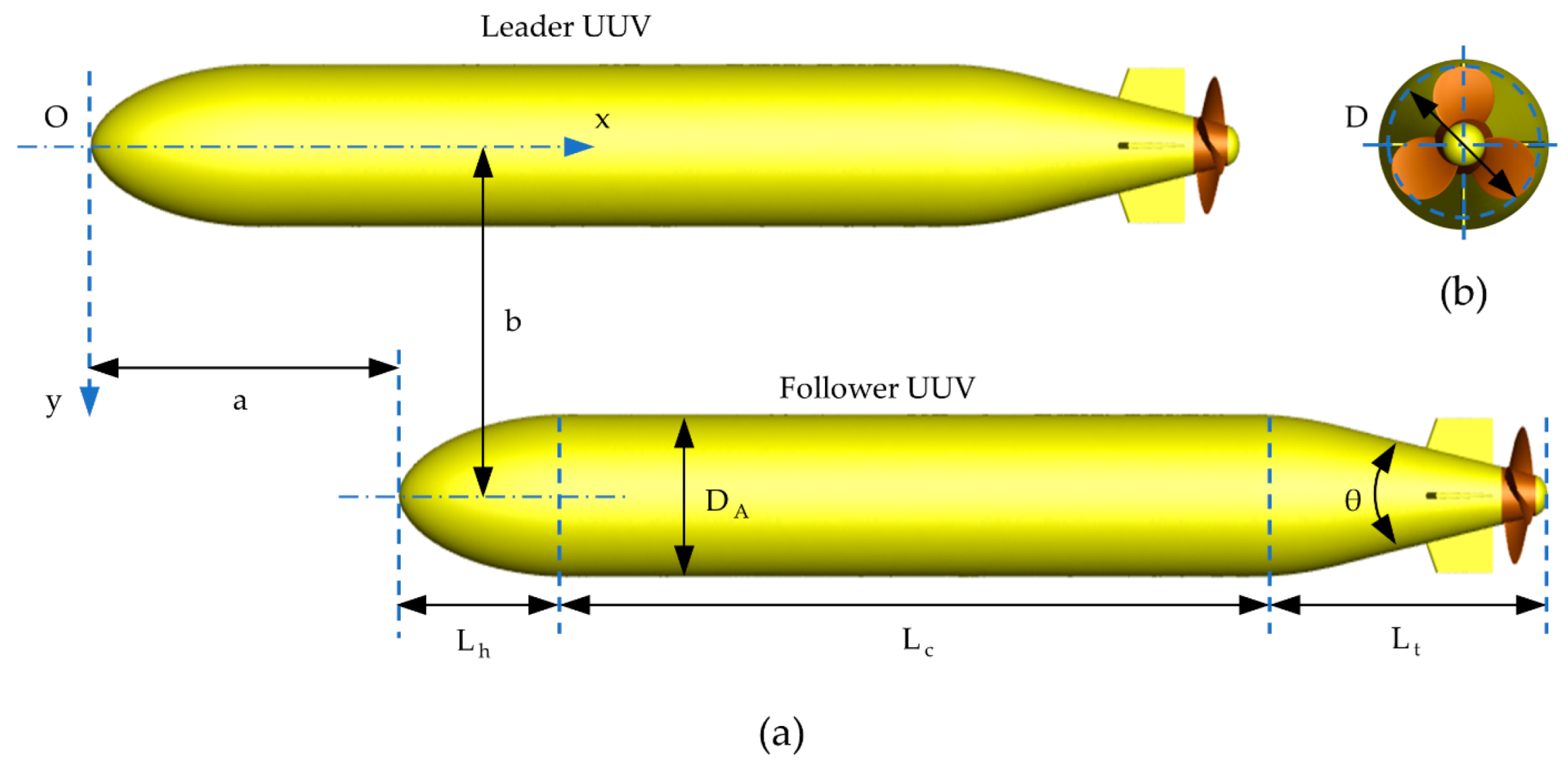
2.1. UUV Geometry Parameters

The self-propelled UUV employed within a multi-UUV vehicle formation comprises three integral components: the hull, the finned rudder plate, and the propeller, as illustrated in Figure 2. The hull’s profile curve is generated based on Equation (1) [23]. The overall length of the UUV is 2 m, and the specific dimensional parameters are detailed in

Table 1. Main parameters of UUV hull and UUV formation.

Parameter	Value	Parameter	Value
$D_A$	0.2 m	$L_t$	0.5 m
$L_A$	2 m	$\mathsf{\theta }$	20°
$L_h$	0.3 m	$a$	Variable
$L_c$	1.2 m	$b$	Variable

. The fin plate’s cross-section adopts a flat plate airfoil with a leading radius of 8 mm. The trailing edge of the fin plate is positioned 1925 mm from the UUV’s nose. In the propeller section, a DTMB4119 model propeller is selected. The propeller dimensions are scaled down to 60% of the original model to accommodate the UUV’s tail section, and corresponding adjustments are made to the hub. Detailed parameters of the propeller are outlined in

Table 2. Detailed parameters of the propeller DTMB4119.

DTMB 4119 Model Propeller
D (m)	0.1829
Z	3
Skew (o)	0
Rake (o)	0
Blade section	NACA66 a = 0.8
Rotation direction	Right
Scaling	0.6

. Notably, the parameters “$a$” and “$b$” play a pivotal role in determining the relative distance between the UUVs.

$$\mathrm{r}\left(x\right)=\frac{1}{2}\mathrm{D}{\left[1-{\left(\frac{x-L_h}{x}\right)}^2\right]}^{1/1.8}$$

(1)

2.2. Definition of Dimensionless Parameters

The following dimensionless parameters are introduced to streamline the problem’s description and analysis. The Reynolds number ($R_e$) is a dimensionless parameter that measures the relative importance of the inertial and viscous forces of the fluid. It is defined as the ratio of the maximum UUV diameter ($D_A$) multiplied by the fluid velocity to the fluid kinematic viscosity. In this study, the Reynolds number ($R_e$) of the oncoming flow is introduced, which is specified as $1.003\times {10}^6$.

$$R_e=\frac{V{D}_A}{\mathsf{\nu }}$$

(2)

The dimensionless distance parameters “$a$” and “$b$”, representing the relative separation between the leader UUV and the follower UUV, are defined using Equations (3) and (4). A cartesian coordinate system is established with the leader UUV’s nose as the origin, where “$x_f$” and “$y_f$” denote the follower UUV’s coordinates. For normalization, the UUV’s axial length $L_A$ is used in the lateral direction, and its maximum diameter $D_A$ is used longitudinally in the equation denominator. These dimensionless parameters take values within the range specified in

Table 3. Value range of dimensionless parameters $a$ and $b$.

Dimensionless Parameters	Description	Range of Values
$a$	Horizontal relative distance	(0, 0.03, 0.06, 0.12, 0.2, 0.4, 0.6, 0.8, 1, 1.1, 1.2, 1.4, 1.6, 1.8, 2, 2.4)
b	Vertical relative distance	(0, 0.2, 0.6, 1, 1.5, 2, 3, 4, 5, 6)

, excluding values corresponding to physical interference distances between UUVs.

$$\mathrm{a}=\frac{\mathrm{x}{ }_{\mathrm{f}}}{{\mathrm{L}}_{\mathrm{A}} }$$

(3)

$$b=\frac{{\mathrm{y}}_f}{D_A}$$

(4)

Furthermore, the subsequent sections of this article provide a detailed discussion of the dimensionless parameters that characterize UUVs’ hydrodynamic performance, including $C_{dl}$, $C_{df}$, and $C_{d0}$, as introduced earlier.

3. Numerical Methods

The paper employs the SST-kw turbulence model and utilizes the ANSYS Fluent 17.0 CFD solver to solve the N-S governing equations. The study utilizes the pressure-based solution approach with a pressure–velocity-coupled solution. The spatial discretization method employs the least squares method for gradients, a second-order format for pressure, and a second-order windward format for the momentum equation, turbulent kinetic energy, and dissipation rate equations. The numerical model must meet certain convergence criteria, whereby the net inlet and outlet flows constitute 10⁻⁶ of the inlet flow, and the relative error of the monitored quantities after two-hundred-step intervals stays within 0.01%. This computational approach is employed to determine the hydrodynamic coefficients for both the individual UUV and the UUV formation. To validate the precision and dependability of the numerical model for the individual UUV, a comparative analysis was conducted, involving a thorough comparison of the numerical results with existing experimental data. This aspect of the research is comprehensively addressed in Section 3.4.

3.1. Governing Equations

This study used Reynolds-averaged Navier–Stokes equations for the three-dimensional incompressible flow, comprising the continuity and momentum equations. These equations are presented below:

$$\frac{\partial \rho }{\partial t}+\frac{\partial \rho {\overline{u}}_i}{\partial t}=0$$

(5)

$$\begin{array}{c}\frac{\partial }{\partial t}\left(\rho {\overline{u}}_i\right)+\frac{\partial }{\partial t}\left(\rho {\overline{u}}_i{\overline{u}}_j\right)=-\frac{\partial P}{\partial x_i}+\frac{\partial }{\partial x_j}\left[\mu \left(\frac{\partial {\overline{u}}_i}{\partial x_j}+\frac{\partial {\overline{u}}_j}{\partial x_i}-\frac{2}{3}{\delta }_{ij}\frac{\partial {\overline{u}}_l}{\partial x_l}\right)\right]\\ -\frac{\partial }{\partial x_j}\left(\rho \overline{u_i^{,}{u}_j^{,}}\right)+F_i\end{array}$$

(6)

The fluid velocity component, denoted as ${\overline{u}}_i$, is governed by the dynamic viscosity coefficient $\mathsf{\mu }$, total pressure $P$, and volume force $F_i$. For simulating the turbulence term within the RANS equations, we employed the SST-kw turbulence model, known for its proficiency in simulating turbulent shear stress transport and delivering accurate predictions of flow separation, even under conditions of inverse pressure gradients. Calculations for turbulent kinetic energy and the turbulent dissipation rate are as follows: $G_k$ and $G_w$ signify the generation terms for turbulent kinetic energy and dissipation rate, respectively, resulting from the mean velocity gradient.

$$\frac{\partial }{\partial t}\left(\rho k\right)+\frac{\partial }{\partial x_i}\left(\rho k{u}_i\right)=\frac{\partial }{\partial x_j}\left({\mathsf{\Gamma }}_k\frac{\partial k}{\partial x_j}\right)+G_k-Y_k+S_k$$

(7)

$$\frac{\partial }{\partial t}\left(\rho w\right)+\frac{\partial }{\partial x_i}\left(\rho w{u}_i\right)=\frac{\partial }{\partial x_j}\left({\mathsf{\Gamma }}_w\frac{\partial w}{\partial x_j}\right)+G_w-Y_w+D_w{+S}_w$$

(8)

In establishing a benchmark for multi-UUV hydrodynamic modeling, it is imperative to create a self-propelled hydrodynamic model for a single UUV. This paper employs the DE-FINE_ZONE_MOTION macro along with the FRM model to iteratively adjust the propeller rotation speed until equilibrium—where the propeller thrust equals the drag force acting on the self-propelled UUV—is achieved. Subsequently, the final propeller rotation speed is determined, and the drag coefficient for the single UUV in self-propelled mode is obtained. The formula for calculating the propeller’s rotational speed is provided below. Maintaining uniform propeller rotational speeds between the UUV formation hydrodynamic model and the single UUV model, the drag coefficient of the single UUV serves as a benchmark for investigating the impact of relative distance on the hydrodynamic performance of the UUV in multi-UUV formations.

$$n=n^{,}+\frac{F_{uuv}+F_{balde}}{F_{uuv}}{\delta }_n$$

(9)

$n^{\prime }$ represents the current speed, $F_{uuv}$ denotes the drag acting on the UUV with the propeller removed, $F_{blade}$ signifies the thrust generated by the propeller, and ${\delta }_n$ represents the convergence factor.

3.2. Computational Domain and Boundary Conditions

Figure 3 illustrates the computational domain of the numerical model, which comprises three parts: one stationary and two rotational domains. The cross-section of the steady-state domain is square, with a length and width of 30 $D_A$. The flow domain length is 12 $L_A$, and the UUV nose is positioned 3 $L_A$ from the inlet boundary to ensure the sufficient development of upstream oncoming and wake flows, reducing numerical modeling errors. The rotating domain takes the form of a cylinder with a diameter of 200 mm and a length of 60 mm. Flow field information transfer between the stationary and rotating domains is facilitated through the use of the INTERFACE. The parameters $a$ and $b$ are used to define the relative distance between the UUVs.

Correct boundary conditions are crucial for the accurate calculation. As a result, the numerical model employs the following boundary conditions:

Inlet: utilizes a velocity inlet condition.

Outlet: implements a pressure outlet condition.

Non-slip walls: applied to the hull, fins, propeller, and underwater walls.

Sliding Walls: utilized for the top and bottom boundaries of the flow domain.

Symmetric Boundaries: employed for the lateral boundaries of the flow domain.

3.3. Meshing Settings

Ansys Fluent Mesh is utilized to discretize the mesh within the computational domain. A hybrid mesh, consisting of both polyhedral and hexahedral elements, is employed for the stationary domain, while the rotational domain utilizes a polyhedral mesh, as demonstrated in Figure 4. This choice is motivated by the polyhedral mesh’s ability to conform to the geometric model’s surface, reducing mesh complexity, along with the excellent orthogonality performance of hexahedral elements.

To ensure the efficient and accurate predictions of the hydrodynamic properties of the UUV and the propeller, two layers of refined regions are strategically positioned around both the UUV and the propeller, as depicted in Figure 4a. Figure 4b illustrates the mesh surrounding the UUV’s nose, while Figure 4c showcases the mesh encompassing the UUV’s tail and the rotational domain. For a precise representation of the propeller’s geometry, a mesh size of 0.05 mm is applied to its leading and trailing edges, as seen in Figure 4d.

To meet the turbulence model’s specifications, prism meshes are generated along all non-slip boundaries within the flow field region, carefully controlling the height of the first mesh layer denoted as Y+ to maintain an approximate value of 1. A total of 15 boundary layers are incorporated into the computational model.

A grid-independent validation assessment was conducted to ascertain the numerical results’ insensitivity to the grid density. Three distinct grid resolutions, specifically 3.2 million (coarse grid), 6 million (medium grid), and 8.4 million (fine grid), were employed for the scenario involving multiple UUVs with parameters $a$ of 0.4 and b of 2. The inflow velocity was maintained at 5 m/s.

Table 4. Grid-independence verification.

Mesh	${\mathit{C}}_{\mathit{d}\mathit{l}}$	${\mathit{C}}_{\mathit{d}\mathit{f}}$
Coarse	0.0045	0.005
Medium	0.0034	0.0036
Fine	0.0033	0.0034

provides a summary of the numerical results obtained at varying grid resolutions. The results obtained with fine and medium meshes exhibit relatively close agreement, suggesting that further increasing the mesh density is unlikely to significantly impact CFD numerical outcomes. Consequently, the medium-resolution mesh is consistently used for all subsequent multi-UUV simulation cases to ensure result consistency and eliminate the influence of varying mesh resolutions on the outcomes.

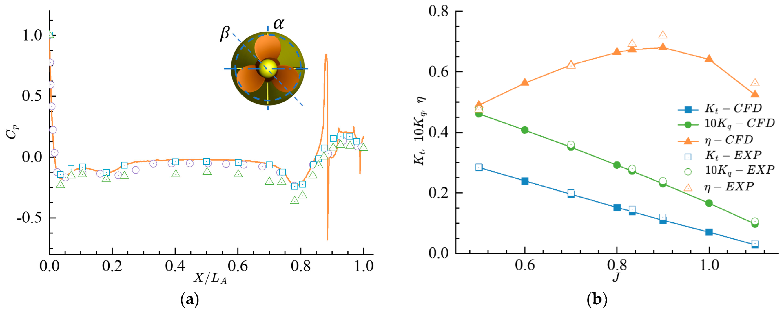
3.4. Verification of Numerical Method

Given the absence of accessible experimental data for self-propelled unmanned underwater vehicles (UUVs), this study conducts numerical simulations of both the UUV and its propeller. The aim is to predict the hydrodynamic attributes of the UUV and the propeller’s performance in open water. These simulations validate the suitability of the numerical methodology employed in this research.

To validate the hydrodynamic characteristics of the UUV, the study opts for the AFF-3 model within the SUBOFF framework as the chosen validation algorithm. This choice is made to confirm the suitability of the numerical approach. The AFF-3 model represents an axisymmetric submarine, and it has been the subject of numerous hydrodynamic tests conducted at the David Taylor Research Center. This database has been made available for validating computational fluid dynamics (CFD) models and conducting flow field analyses related to submarines. Consequently, many scholars have adopted the SUBOFF framework for UUV research.

For instance, Huang et al. [24] conducted experimental research on the hydrodynamic performance of the AFF-8 model using a Reynolds number $R{e}_L$ of 12 × 10⁶. Jiménez et al. [25] investigated the wake characteristics of the AFF-2 model using a $R{e}_L$ of 1.1 × 10⁶ through wind tunnel tests. Additionally, Posa et al. [13] studied the turbulent boundary layer on the surface of the AFF-8 model using a $R{e}_L$ of 1.2 × 10⁶ using CFD methods. These studies provided valuable insights into the distribution of pressure coefficients ($C_p$) on the UUV’s surface at a $R{e}_L$ of 1.2 × 10⁶, as determined through CFD simulations.

$$C_p=\frac{P-P_0}{\frac{1}{2}\rho V_0^2}$$

(10)

$C_p$ is determined using Equation (10). Figure 5a presents a comparison of the numerical results. The validation results closely align with Huang et al.’s experimental findings and are consistent with the trends observed by other researchers. Notably, a deviation in $C_p$ from the results of other researchers is evident near the fin plate of the model, as illustrated in Figure 5a. This deviation can be attributed to two primary factors: (1). Discrepancies in the geometric model, particularly the absence of a fin rudder in Jiménez’s numerical model. (2). Variation in the pressure observation cross-section on the UUV: Huang and Posa’s observations are based on a 45° longitudinal profile $\beta$ between the fin rudder, whereas the validation calculations in this paper utilize a 0° longitudinal profile $\alpha$ passing through the center profile of the fin rudder. These differences in geometric modeling and observation of cross-section locations lead to variations in the pressure coefficient distribution along the leading edge of the fin plate.

The DTMB 4119 propeller has found extensive application in research about non-cavitation propeller vibration, cavitation performance, and cavitation noise. Additionally, it has served as a benchmark for numerous researchers seeking to validate the reliability of numerical methods. Validation efforts involving computational fluid dynamics (CFD) were conducted using the DTMB 4119 propeller, yielding open-water performance characteristics that were subsequently compared to experimental data. As depicted in Figure 5b, the numerical results exhibit a strong agreement with the experimental findings. Notably, the most significant discrepancy is observed in the efficiency parameter, with a value of $J$ equaling 0.833 and a relative error of 2.57%. This discrepancy indicates that the numerical method diverges slightly from the simulation results towards the experimental results at high Reynolds numbers, albeit remaining within an acceptable range. It is imperative to note that the experimental results for this propeller were graciously provided by Jessup [26]. This work is licensed under Attribution 4.0 International.

4. Results and Discussion

4.1. Single Propeller UUV Numerical Simulation Results

Numerical modeling tests are first performed on a single self-propelled UUV equipped with a propeller as a comparative benchmark for the hydrodynamic performance of multiple UUVs. The rotational speed of the propeller is varied until the drag of the UUV is equal to the thrust of the propeller by fixing the incoming flow rate. This iteration process of UUV propeller drag is shown in Figure 6a, where the horizontal coordinate N of the inset represents the number of iterative steps. From the figure, it can be seen that there is a gradual increase in the thrust of the propeller as the number of iterations is increased. This is due to the progressive increase in the rotational speed of the propeller. The drag of the UUV increases slowly. The presence of the propeller at the tail of the UUV leads to an increase in the velocity of the flow field at the tail and a decrease in the pressure field, which, in turn, leads to an increase in the drag of the UUV, corresponding to the thrust reduction phenomenon of the propeller. After about 3000 increments, the resistance of the UUV begins to match the thrust of the propeller. Figure 6b shows the time history curve of the propeller speed, from which it can be seen that the rotational speed of the propeller gradually increases, verifying the propeller thrust’s gradually increasing trend that is shown in Figure 6a. After stabilizing the calculation, the final propeller speed is 1447.3 rpm, and the UUV drag after excluding the propeller thrust is 54 N.

4.2. Numerical Results of the Hydrodynamic Test of the UUV Formation

To facilitate a comparison and discussion, this paper expresses the UUV’s resistance in dimensionless terms. Herein, $C_{dl}$ and $C_{df}$ denote the resistance coefficients for the leader UUV and the follower UUV, respectively. Within the formulas, $F_{xl}$ and $F_{xf}$ represent the drag of the UUV, with $\mathsf{\rho }$ denoting the fluid density ($\mathsf{\rho }=998.2\mathrm{k}\mathrm{g}/{\mathrm{m}}^3$) and $S$ indicating the UUV’s wetted surface area. These formulas are employed to compute the drag coefficient for an individual UUV. It is important to emphasize that the resistance values in these equations exclude the propeller thrust and exclusively account for the combined resistance arising from the hull of the navigating UUV and the fin rudder. Furthermore, $C_{d0}$ designates the drag coefficient of a single UUV.

$$C_{dl}=\frac{F_{xl}}{\left(1/2\right)\mathsf{\rho }S{V}^2}$$

(11)

$$C_{df}=\frac{F_{xf}}{\left(1/2\right)\mathsf{\rho }S{V}^2}$$

(12)

$$C_{d0}=\frac{F_x}{\left(1/2\right)\mathsf{\rho }S{V}^2}$$

(13)

The parameters $r_l$ and $r_f$ signify the relative increment in the drag coefficient for the leading and following UUVs within a UUV formation, as compared to that of a solitary UUV.

$$r_l=\frac{C_{dl}-C_{d0}}{C_{d0}}$$

(14)

$$r_f=\frac{C_{df}-C_{d0}}{C_{d0}}$$

(15)

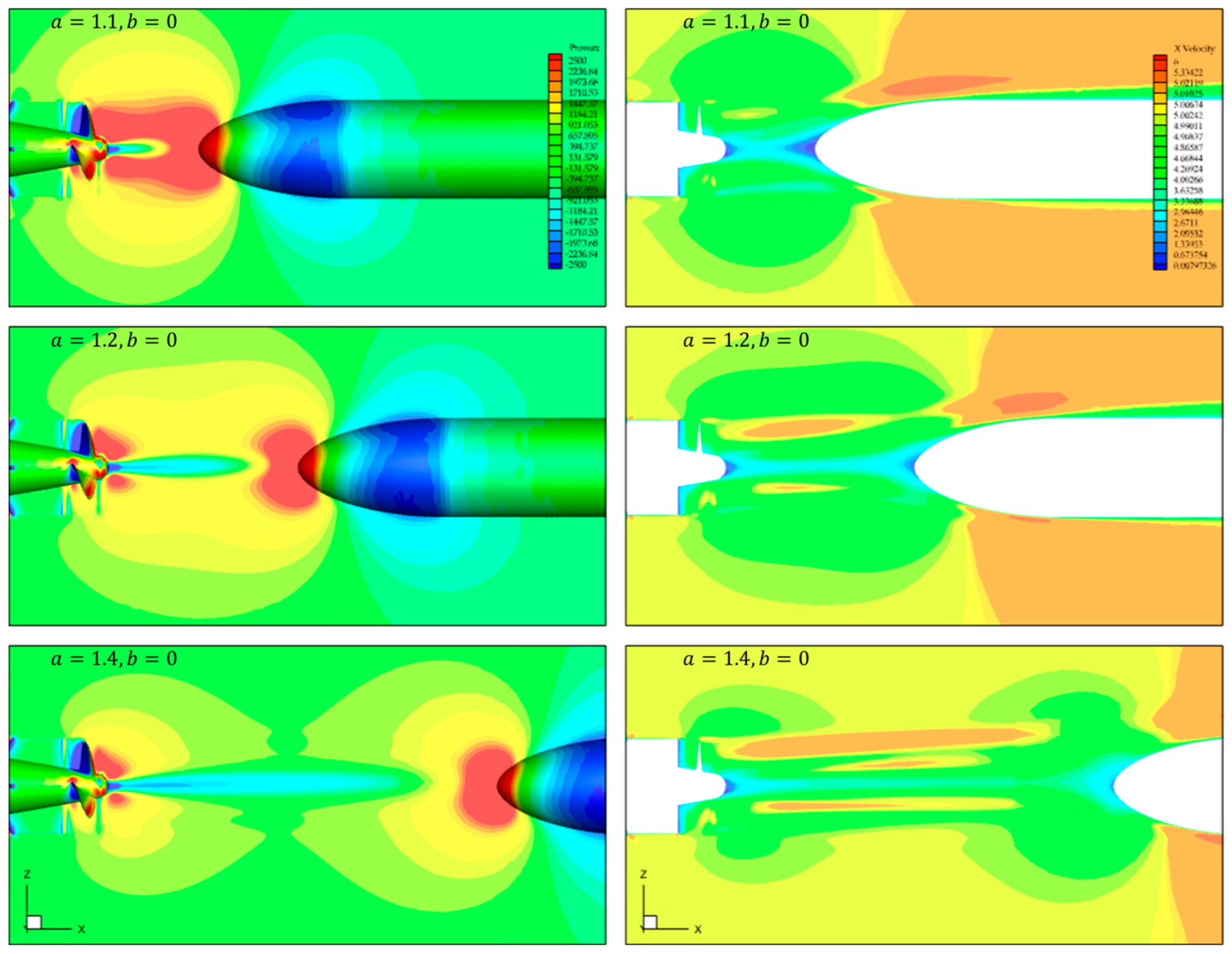
4.2.1. Influence of a UUV’s Relative Distance on Hydrodynamic Performance

The hydrodynamic performance of both the leader and follower UUVs within the UUV formation is influenced by their interactions, leading to variations in their respective drag coefficients. As depicted in Figure 7, the heat map illustrating the relative drag coefficients of the leader UUV and the follower UUV predominantly reveals two distinct regions: the “pull” region and the “push” region. Other regions emerge due to increased relative distances between UUVs within the formation, where mutual interference effects between UUVs become negligible. Remarkably, the pull and push regions of the leader UUV exhibit substantial overlap with those of the follower UUV, lending support to the accuracy of the numerical model employed. Notably, the distribution ranges of these pull and push regions broadly align with the findings reported by Tian et al. [22].

Within the pull region, the high-pressure regions at the front of both the leader and follower UUVs converge, as do the low-pressure regions along their parallel sections and the high-pressure regions at their respective tails. These factors result in an attractive force between the leader and follower UUVs, driven by the combined influence of high-pressure zones at the front and rear and low-pressure zones along the parallel sections. The positive value of $r_l$ for the leader UUV signifies an increase in its drag coefficient relative to that of an individual UUV when coupling forces are present. Conversely, the negative value of $r_f$ for the follower UUV indicates a decrease in its drag coefficient relative to that of an individual UUV under the influence of coupling forces.

In the push region, the pressure fields at the head and parallel section of the leader UUV remain largely unaffected by the presence of the follower UUV. However, the high-pressure region, in the wake of the leader UUV, coincides with the high-pressure region at the head of the follower UUV, intensifying the pressure distribution in this area. Consequently, the leader UUV and the follower UUV experience repulsive forces, with $r_l$ being negative for the leader UUV, indicating a decrease in its drag coefficient relative to an individual UUV. Conversely, $r_f$ is positive for the follower UUV, indicating an increase in its drag coefficient relative to an individual UUV. This phenomenon is elucidated in Figure 8.

Furthermore, as observed in Figure 7, within the pull region, $r_l$ for the leader UUV exhibits an approximate trend of first increasing and then decreasing in the ‘a’ direction; meanwhile, the corresponding $r_f$ for the follower UUV undergoes an approximate trend of first decreasing and then increasing. Figure 9 illustrates the pressure and velocity fields when the UUVs are in the pull region, with ‘$b$’ equal to 1.5 and ‘$a$’ values of 0.03, 0.12, and 0.4. As ‘$a$’ increases. The high-pressure regions at the head and wake of the formation gradually separate, weakening the forces between the UUVs. Simultaneously, the force direction between the UUVs progressively biases toward the ‘$a$’ direction, akin to the decreasing trend observed in Figure 9. This trend positively contributes to the ‘$a$’-directional force component between the UUVs, explaining the trends in $r_l$ for the leader UUV and $r_f$ for the follower UUV in the ‘$a$’ direction.

For the $b$ direction, the $r_l$ for the leader UUV steadily decreases, and the corresponding $r_f$ for the follower UUV consistently increases. Figure 10 illustrates pressure and velocity distributions within the pull region for ‘a’ equal to 0.12 and ‘b’ values of 2, 4, and 6. As the ‘b’ direction distance increases, the high-pressure regions at the head and wake of the formation, as well as the low-pressure regions along the parallel section, gradually separate. Consequently, the forces between the UUVs weaken. Concurrently, the force direction between the UUVs increasingly biases toward the ‘b’ direction, as depicted in Figure 10. The angle θ progressively increases, contributing positively to a reduction in the ‘$a$’-directional force component between the UUVs, further diminishing the force components in the ‘a’ direction. These trends elucidate the behavior of $r_l$ for the leader UUV and $r_f$ for the follower UUV in the ‘b’ direction. Remarkably, the trends in $r_l$ and $r_f$ with ‘a’ and ‘b’ align with the findings in Tian’s article within the pull region [22].

In the pull region, the maximum value of $r_l$ is 31.23%, while the minimum value of $r_f$ is −20.9%. This occurrence arises when ‘$a$’ equals 0.12 and ‘$b$’ equals 1.5.

Within the push region, both $r_l$ values for the leader UUV in the ‘$a$’ and ‘$b$’ directions exhibit progressive increments, while the corresponding $r_f$ values for the follower UUV undergo gradual reductions. Illustrated in Figure 11 are the pressure and velocity fields of the UUV formation within the push region, with ‘$b$’ set to 0 and ‘$a$’ values of 1, 1.2, and 1.4. As depicted in the figure, the high-pressure zones in the wake of the leader UUV and at the nose of the follower UUV gradually separate as the ‘$a$’-direction distance increases, resulting in a diminishing force between the UUVs. Remarkably, the evolution of the pressure and velocity fields in the ‘$b$’ direction, as shown in Figure 12, closely mirrors that observed in the ‘$a$’ direction.

In the push region, the maximum value of $r_f$ reaches 22.03%, while the minimum value of $r_l$ is −12.2%. This scenario occurs when ‘$a$’ is 1.1 and ‘$b$’ is 0.2.

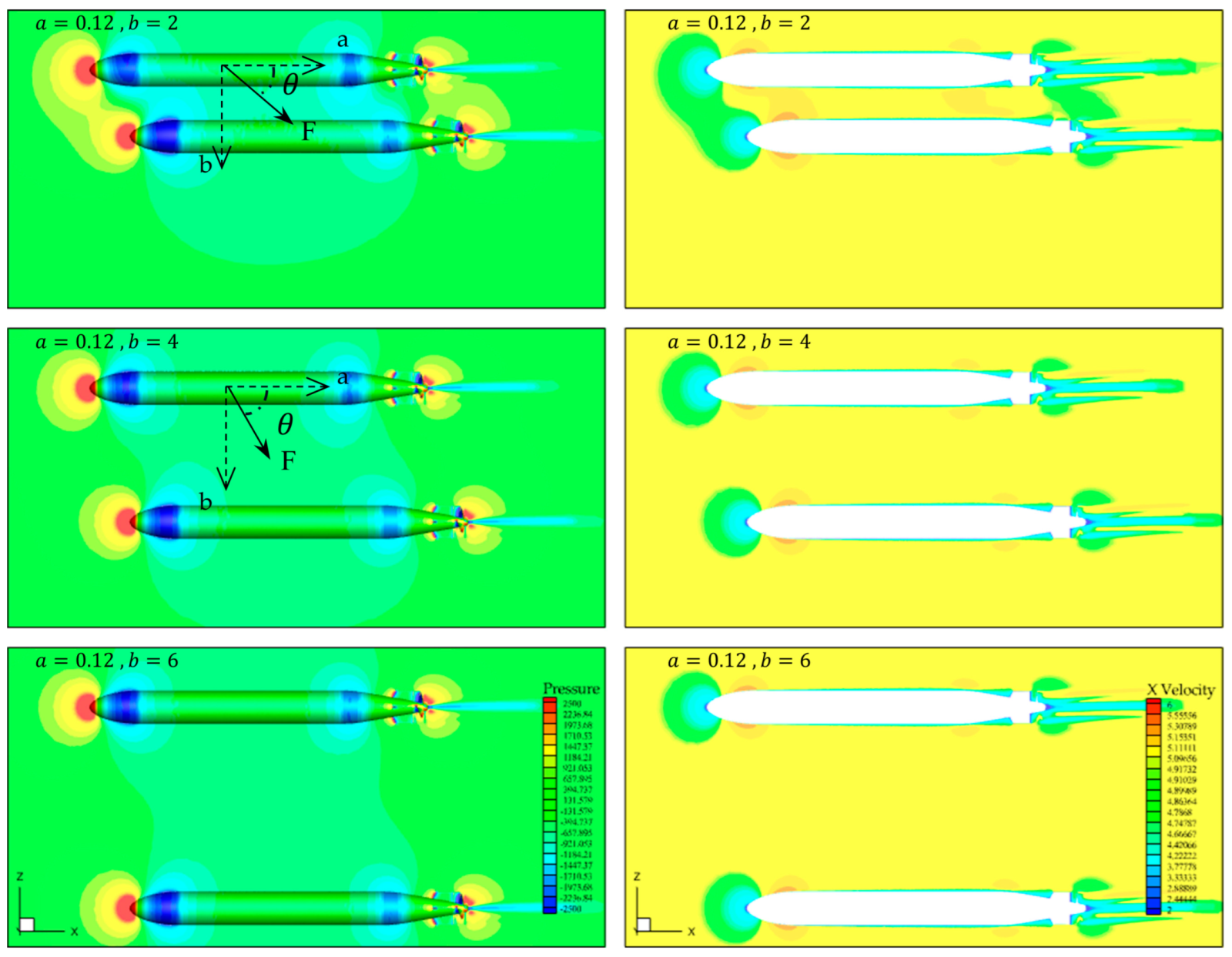
4.2.2. Influence of a UUV’s Relative Distance on Hydrodynamic Performance

To analyze the impact of relative distance on the overall hydrodynamics of a formation of UUVs, this article introduces the parameter $R_{fleets}$. This parameter represents the hydrostatic thrust of the UUV formation to a self-propelled UUV, which possesses zero hydrostatic thrust. In essence, $R_{fleets}$ accounts for the cumulative effect of drag and thrust generated by the UUVs within the formation. The thrust of the leading and trailing propellers in Equation (16) is represented by $T_l$ and $T_f$.

$$R_{fleets}=T_l-F_{xl}+T_f-F_{xf}$$

(16)

The static thrust of the UUV formation remains at zero when the value of $R_{fleets}$ is 0, indicating no improvement in drag performance compared to a single UUV. However, when $R_{fleets}$> 0, it signifies that the total thrust generated by the UUVs within the formation exceeds the total drag, implying the superior performance of the UUV formation compared to a single UUV. This advantage is influenced by the relative distance between the UUVs in the formation. Conversely, when $R_{fleets}$< 0, the hydrodynamic performance of the UUV formation falls below that of a single UUV, as the total thrust from the propellers in the UUV formation is less than the total drag of the UUVs.

In Figure 13, it is evident that the hydrostatic thrust of the UUV formation peaks at 3.76 N, which is 7% greater than the drag of self-propelled UUVs. This occurs when the relative distances ’$a$’ and ‘$b$’ are set at 1.1 and 1, respectively.

5. Conclusions

This paper explores the hydrodynamics of a self-propelled UUV. The study involves a self-propelled UUV experiencing a drag force of 54 N and a propeller rotational speed of 1447.3 rpm within an oncoming flow characterized by a Reynolds number ($R_e$) of $1.003\times {10}^6$. The primary focus of this research is to analyze the correlation between the relative distances among UUVs within a formation and the resulting hydrodynamic performance of the formation.

The following conclusions can be drawn from this study:

• When analyzing the drag coefficient of an individual UUV within a formation, the map depicting relative distances primarily divides into pull and push regions. The extreme values of $r_l$ and $r_f$ in the heat map are located in the same position;
• In the pull region, the high-pressure areas at the head and tail of the formation are gradually separated as the “a” value increases; meanwhile, the direction of the force between UUVs is gradually biased towards the “a” direction, and the force between UUVs is weakened. The $r_l$ of the leading UUV shows an approximate increasing and then decreasing trend in the “a” direction, while the corresponding $r_f$ of the following UUV shows an approximate decreasing and then increasing trend. Along the “b” direction, as the distance increases, the high-pressure zones at the head and tail of the formation and the low-pressure zones in the parallel profile are gradually separated, while the direction of the force between the UUVs is gradually biased toward the “b” direction, and, thus, the force between the UUVs is weakened. The leading UUV experiences a steady decrease in $r_l$, while the corresponding $r_f$ of the following vehicles continues to rise. In the push region, the high-pressure areas at the rear of the leading UUV and the front of the following UUV separate slowly as the distance between the “a” and “b” directions increases, leading to a progressive reduction in the force between the UUVs. The $r_l$ values of the leading UUV in both “a” and “b” directions show a tendency to gradually increase, while the corresponding $r_f$ values of the following UUV gradually decrease.
• In vehicle formations, a positive static thrust area is present when two vehicles are arranged in a staggered position. As the relative distance increases, the static thrust value declines.

This study is limited to a specific $R_e$ value of 1.003 × 10⁶. Subsequent research may investigate the impact of varying $R_e$ on the interdependent hydrodynamic performance of multi-vehicle formations, laying the groundwork for the development of formation control systems.

References

1. Liu, X.; Hu, Y.; Mao, Z.; Tian, W. Numerical Simulation of the Hydrodynamic Performance and Self-Propulsion of a UUV near the Seabed. Appl. Sci. 2022, 12, 6975. [Google Scholar] [CrossRef]
2. Cao, X.; Guo, L. A leader-follower formation control approach for target hunting by multiple Autonomous Underwater Vehicles in Three-Dimensional Underwater Environments. Int. J. Adv. Robot. Syst. 2019, 16, 1729881419870664. [Google Scholar] [CrossRef]
3. Zhao, P.; Li, J.; Mao, Z.; Ding, W. Cooperative Search Path Planning for Multiple Unmanned Surface Vehicles. In Proceedings of the 2022 International Conference on Autonomous Unmanned Systems (ICAUS 2022); Springer Nature: Singapore, 2023; pp. 3434–3445. [Google Scholar]
4. Zhang, L.C.; Xu, S.F.; Liu, M.Y.; Xu, D.M. Progress in cooperative navigation and localization of multiple unmanned underwater vehicles (UUVs). High-Tech Commun. 2016, 26, 475–482. [Google Scholar]
5. Xie, Q.L.; Song, L.; Lu, H.; Zhou, B.C.H. Synthesis of research on cooperative navigation techniques. Aero Weapon. 2019, 26, 23–30. [Google Scholar]
6. Wang, Y.T.; Yan, W.S. Consensus formation tracking control of multiple autonomous underwater vehicle systems. Control. Theory Appl. 2013, 30, 379–384. [Google Scholar]
7. Zeng, B.; Zhang, H.Q.; Li, H.P. Research on anti-submarine strategy for unmanned undersea vehicles. Syst. Eng. Electron. 2022, 44, 3174–3181. [Google Scholar]
8. Xie, W.; Tao, H.; Gong, J.B.; Luo, W.; Yin, F.; Liang, X. Research advances in the development status and key technology of unmanned marine vehicle swarm operation. Chin. J. Ship Res. 2021, 16, 7–17, 31. [Google Scholar] [CrossRef]
9. Jagadeesh, P.; Murali, K.; Idichandy, V.G. Experimental Investigation of Hydrodynamic Force Coefficients over AUV Hull Form. Ocean. Eng. 2009, 36, 113–118. [Google Scholar] [CrossRef]
10. Guo, C.Y.; Zhao, Q.X.; Zhao, D.G. Data Processing Method of Self-propulsion Test of Ship Based on CFD. Ship Ocean. Eng. 2013, 42, 17–20. [Google Scholar]
11. Vali, A.; Saranjam, B.; Kamali, R. Experimental and Numerical Study of a Submarine and Propeller Behaviors in Submergence and Surface Conditions. JAFM 2018, 11, 1297–1308. [Google Scholar] [CrossRef]
12. Zhang, R.; Dong, X.; Wang, Z.; Huang, Y.; Yu, J. Numerical Design and Validation of Propeller for Long-range AUV. China Shipbuild. 2019, 60, 141–153. [Google Scholar]
13. Posa, A.; Broglia, R.; Felli, M.; Falchi, M.; Balaras, E. Characterization of the Wake of a Submarine Propeller via Large-Eddy Simulation. Comput. Fluids 2019, 184, 138–152. [Google Scholar] [CrossRef]
14. Wang, L.; Martin, J.E.; Felli, M.; Carrica, P.M. Experiments and CFD for the Propeller Wake of a Generic Submarine Operating near the Surface. Ocean. Eng. 2020, 206, 107304. [Google Scholar] [CrossRef]
15. Carrica, P.M.; Kim, Y.; Martin, J.E. Near-Surface Self Propulsion of a Generic Submarine in Calm Water and Waves. Ocean. Eng. 2019, 183, 87–105. [Google Scholar] [CrossRef]
16. Luo, W.; Jiang, D.; Wu, T.; Liu, M.; Li, Y. Numerical Simulation of the Hydrodynamic Characteristics of Unmanned Underwater Vehicles near Ice Surface. Ocean. Eng. 2022, 253, 111304. [Google Scholar] [CrossRef]
17. Yang, G. Asymptotic Tracking with Novel Integral Robust Schemes for Mismatched Uncertain Nonlinear Systems. Intl. J. Robust Nonlinear 2023, 33, 1988–2002. [Google Scholar] [CrossRef]
18. Shi, K.; Wang, X.H.; Xu, H.-X.; Guo, C.-L.; Chen, H. Model-free parameter adaptive sliding mode control for autonomous underwater helicopters. Ship Sci. Technol. 2022, 44, 73–79. [Google Scholar]
19. Li, H.; An, X.; Feng, R.; Chen, Y. Motion Control of Autonomous Underwater Helicopter Based on Linear Active Disturbance Rejection Control with Tracking Differentiator. Appl. Sci. 2023, 13, 3836. [Google Scholar] [CrossRef]
20. Du, P.; Yang, W.; Wang, Y.; Hu, R.; Chen, Y.; Huang, S.H. A Novel Adaptive Backstepping Sliding Mode Control for a Lightweight Autonomous Underwater Vehicle with Input Saturation. Ocean. Eng. 2022, 263, 112362. [Google Scholar] [CrossRef]
21. Molland, A.F.; Utama, I.K.A.P. Experimental and Numerical Investigations into the Drag Characteristics of a Pair of Ellipsoids in Close Proximity. Proc. Inst. Mech. Eng. Part M J. Eng. Marit. Environ. 2002, 216, 107–115. [Google Scholar] [CrossRef]
22. Tian, W.; Mao, Z.; Zhao, F.; Zhao, Z. Layout Optimization of Two Autonomous Underwater Vehicles for Drag Reduction with a Combined CFD and Neural Network Method. Complexity 2017, 2017, 5769794. [Google Scholar] [CrossRef]
23. Joung, T.-H.; Sammut, K.; He, F.; Lee, S.-K. Shape Optimization of an Autonomous Underwater Vehicle with a Ducted Propeller Using Computational Fluid Dynamics Analysis. Int. J. Nav. Archit. Ocean. Eng. 2012, 4, 44–56. [Google Scholar] [CrossRef]
24. Huang, T.; Liu, H.L. Measurements of Flows over an Axisymmetric Body with Various Appendages in a Wind Tunnel: The DARPA SUBOFF Experimental Program; British Maritime Technology: London, UK, 1994. [Google Scholar]
25. Jiménez, J.M.; Hultmark, M.; Smits, A.J. The Intermediate Wake of a Body of Revolution at High Reynolds Numbers. J. Fluid Mech. 2010, 659, 516–539. [Google Scholar] [CrossRef]
26. Jessup, S.D.; Boswell, R.J.; Nelka, J.J. Experimental Unsteady and Time Average Loads on the Blades of the Cp Propeller on a Model of the Dd-963 Class Destroyer for Simulated Modes of Operation; David W. Taylor Naval Ship Research and Development Center: Bethesda, MD, USA, 1977. [Google Scholar]
Figure 1. A flow chart of the research methodology and the contents.
Jmse 11 02088 g001
Figure 2. (a) Schematic diagram of UUV formation; (b) UUV propeller schematic.
Jmse 11 02088 g002
Figure 3. Schematic of the flow field.
Jmse 11 02088 g003
Figure 4. Grid settings: (a) the longitudinal profile grid of the domain; (b) UUV nose grid; (c) UUV tail grid; (d) propeller grid.
Jmse 11 02088 g004
Figure 5. (a) Pressure coefficient of SUBOFF AFF-3: present results, plane on the side of the negative Z axis; ○ Posa et al. [13] at R e L 1.2 × 10⁶; □ Huang et al. [24] (1994) at R e L 12 × 106; △ Jiménez et al. (2010a) [25] at R e L 1.1 × 10⁶. (b) Verification of the open-water performance of DTMB4119.
Jmse 11 02088 g005
Figure 6. (a) UUV hydrodynamic iteration curve; (b) propeller speed–time history curve.
Jmse 11 02088 g006
Figure 7. (a) Heatmap of r l for leader UUVs; (b) heatmap of r f for follower UUVs.
Jmse 11 02088 g007
Figure 8. Distribution of the pressure field around the leader UUV and the follower UUV in a formation of UUVs.
Jmse 11 02088 g008
Figure 9. The pressure cloud and the velocity field for different values of a with b equal to 1.5 in the pull region.
Jmse 11 02088 g009
Figure 10. The pressure cloud and the velocity field for different values of b with a equal to 0.12 in the pull region.
Jmse 11 02088 g010
Figure 11. The pressure cloud and the velocity field for different values of a with b equal to 0 in the push region.
Jmse 11 02088 g011
Figure 12. The pressure cloud and the velocity field for different values of b with a equal to 1.1 in the push region.
Jmse 11 02088 g012
Figure 13. Heatmap of R f l e e t for UUVs.
Jmse 11 02088 g013