Enhanced Mixing Induced by Near-Inertial Waves Inferred by Glider Observation in the Northern South China Sea

Abstract

Enhanced turbulence triggered by near-inertial wave (NIW) trapping by a mesoscale anticyclone and typhoon “Kompasu” was observed in the northern South China Sea. The observations provide evidence for the trapping of NIW packets of amplitude ~0.2 m/s near the base of an anticyclonic eddy, and of ~0.3 m/s after the passage of typhoon “Kompasu”. The wave energy was amplified in a layer located near the base of the anticyclonic eddy, between 150 and 300 m, while stronger NIWs triggered by the typhoon extended to depths > 500 m. Diffusivity was calculated by a fine-scale parameterization. A diffusivity elevated by one order of magnitude, the occurrence of high near-inertial velocity shears, and the low (≤1) Richardson numbers were consistent with turbulence production and mixing from the base of the anticyclonic eddy and following the passage of the typhoon, and were associated with the trapped NIWs. This study showed that, by serving as a bridge between mesoscale eddies and small-scale motion, NIWs are an important pathway for ocean energy transmission. Mesoscale-NIW interactions represent a significant source of NIWs as well as a sink of mesoscale energy.

1. Introduction

The ocean circulation is forced at the basin scale and dissipated at the centimeter scale. The dynamic path from forcing to dissipation runs through all intervention scales, but it poses a fundamental challenge in determinations of the quasi-equilibrium state of the ocean. Mesoscale eddies are the main kinetic energy reservoir in the world’s oceans, as they contain ~90% of the ocean’s kinetic energy [1]. Mesoscale eddies can use the ocean’s internal waves as a “bridge” to provide energy for mixing across equi-density surfaces within the ocean, thus driving the meridional overturning circulation, the transport of low-latitude high temperatures, and the movement of areas of high salinity northward to high-latitude areas. The stored heat is released through the atmosphere, thereby affecting the global climate. Internal mixing of the ocean caused by the breaking of internal waves provides potential energy for low-temperature, high-salinity water in the lower layers of the ocean, which in turn drives the global meridional overturning circulation [2]. In addition, the internal tides and near-inertial internal waves (NIWs) are the other main sources of internal waves. As NIWs are ubiquitous features of the world ocean, they are suggested to play a significant role in deep small-scale mixing [3]. The mechanisms of NIWs and their effectiveness in propagating downward and dissipating their energy and thus inducing small-scale deep mixing is an ongoing issue [4].

NIWs are mainly generated by sea surface winds, initially in the form of near-inertial oscillations in the mixed layer of the sea surface. They are then propagated in the form of waves toward the inner region of the ocean. During this propagation, smaller-scale internal waves are gradually generated, ultimately breaking while driving turbulent mixing in the inner region of the ocean [3,5,6]. Turbulent mixing affects the transport of matter and energy in the ocean, thus playing a crucial role in the formation of ocean circulation and climate [2,7]. Anticyclonic mesoscale eddies can capture NIWs to promote the downward transfer of their energy through an “inertial chimney effect”, which is an important channel for the transmission of wind-induced near-inertial energy to the deep sea to drive turbulent mixing [3]. The traditional view holds that warm eddies promote and cold eddies suppress the downward transfer of near-inertial energy [2,8,9].

The South China Sea (SCS) is the largest semi-enclosed marginal sea in the northwestern Pacific Ocean. Its large-scale currents are driven by the East Asian monsoon [10]. Several multiscale dynamic processes act on the SCS, including wind- and density-driven circulation [11,12], strong internal waves [13,14], enhanced turbulent mixing [15,16], and energetic mesoscale eddies [17,18,19,20]. The SCS is also frequently traversed by tropical cyclones from the northwestern Pacific Ocean; furthermore, it is the origin of local tropical cyclones that are accompanied by strong NIWs [21,22].

In the following, using data from moored current measurements and glider observations, we provide observational evidence of NIW trapping by a mesoscale anticyclone and typhoon “Kompasu” in the northern SCS that was accompanied by strong turbulence. To our knowledge, NIW trapping by mesoscale eddies in the SCS has yet to be demonstrated based on observational data. Our findings suggest that mesoscale-NIW interactions are both a significant source of NIWs and a sink of mesoscale energy in the SCS.

2. Materials and Methods

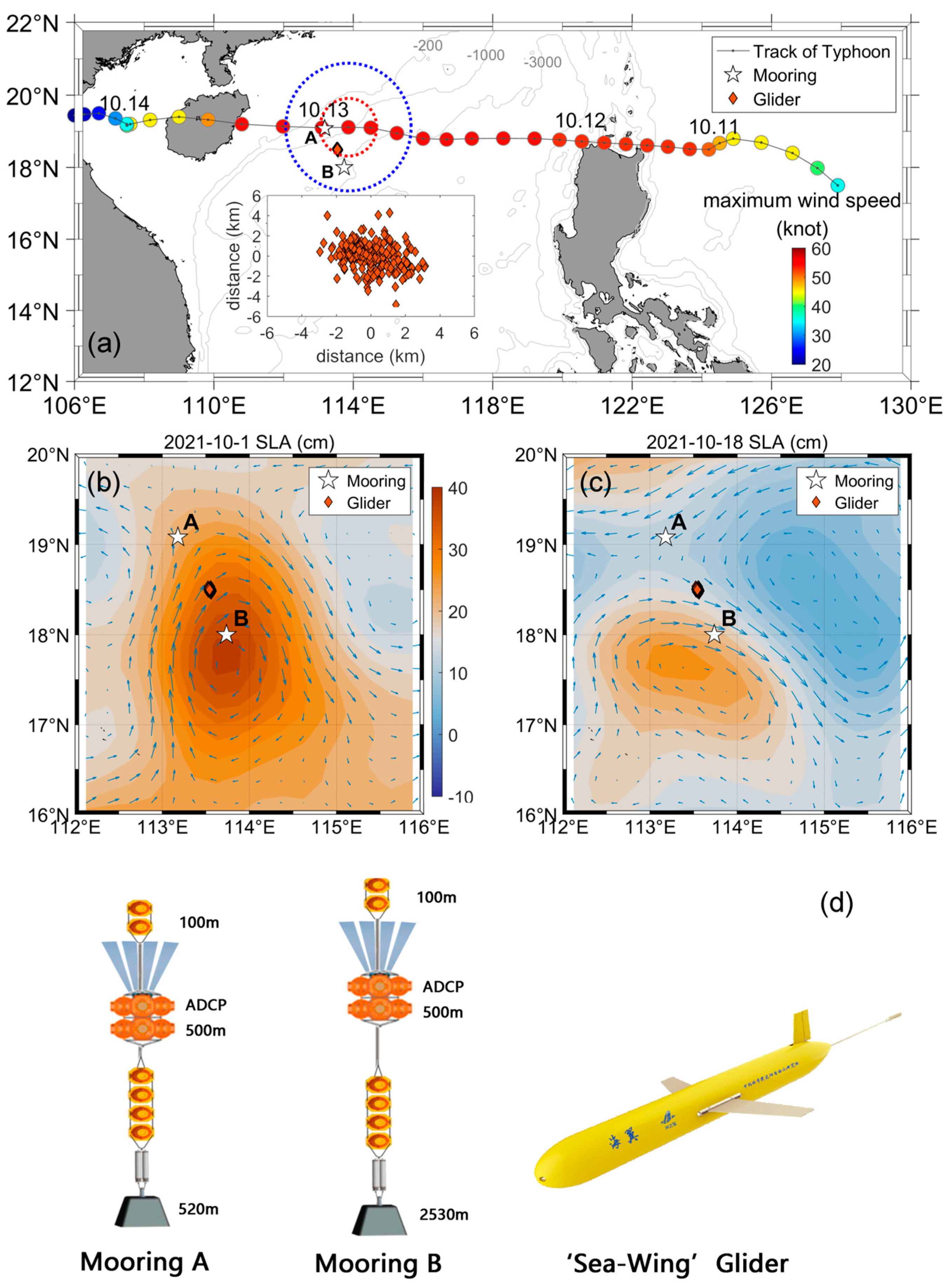
2.1. Mooring Observation

Two moorings were deployed in the northern SCS from 1 October 2021 to 1 November 2021, by the South China Sea Institute of Oceanology (Figure 1). The moorings were located at 113.18° E, 19.07° N (mooring A) and 113.74° E, 18° N (mooring B), at bottom depths of 520 m and 2530 m, respectively. Both were equipped with a 75-kHz RDI acoustic Doppler current profiler (ADCP) at a depth of ~500 m (Figure 1d). The velocity accuracy reaches 1.0% ± 0.5 cm/s of the measured currents. The ADCP was configured to measure the velocity by averaging 10 pings with 2 min in 55 bins with a bin size of 8 m. Acceptable ADCP measurements were first quality-controlled by removing profiles in which the 3-beam solution was <80%, leading to the top bin of the currents approximately equal to 100 m. The pressure record from the pressure sensor mounted on the ADCP was then used to correct the bin depths of the ADCP. Given that the instrument depth fluctuated with time due to the swinging of the moorings, to maintain a consistent depth for the two moorings at different times, all ADCP data were linearly interpolated to fixed 8 m vertical bins.

2.2. Glider Observations

In parallel with the mooring observation, a Chinese underwater glider (Sea-wing, Figure 1d) was deployed between the moorings (Figure 1a–c). The glider was operated in virtual anchoring mode, such that it always moved at the same target position of 18.5° N, 113.5° E. In this operation mode, the surface position of the underwater glider was controlled within 5 km (Figure 1a, inlet). Temperature, salinity, and pressure were measured by a Seabird Glider Payload CTD, with their inertial accuracy reaching ±0.002 °C, ±0.0003 S/m, and ±0.1% of full-scale range, respectively. Dissolved oxygen (DO) was measured by an Aanderaa Oxygen Optode sensor installed on the glider. The glider profiled the water column to a depth of 1000 m and captured 270 vertical temperature and salinity profiles within one month.

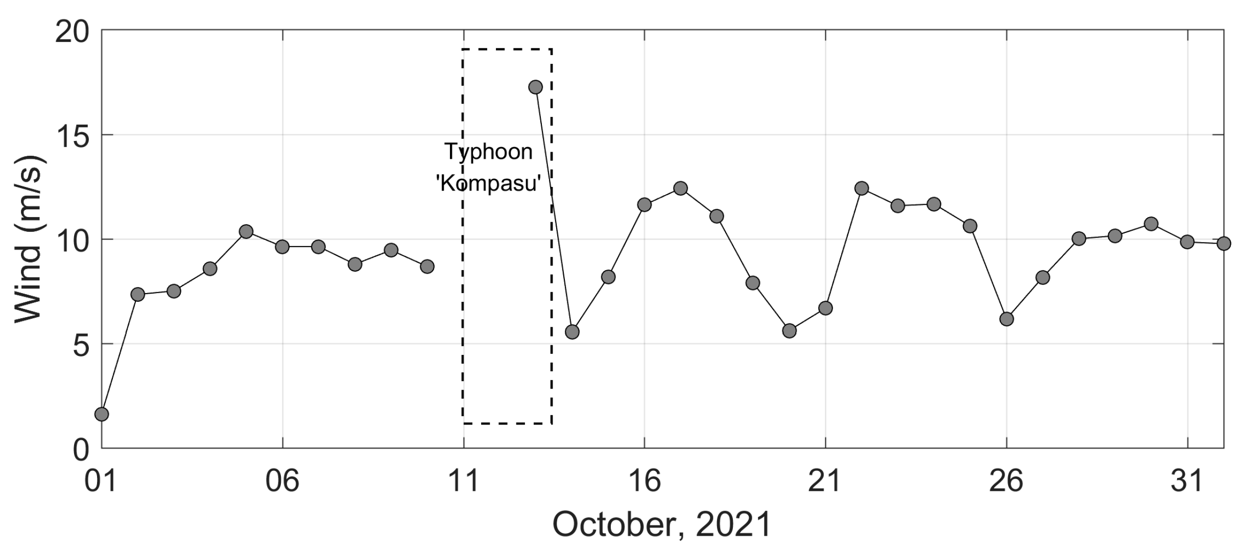
2.3. Typhoon and Wind Information

Typhoon “Kompasu” developed in the Northwest Pacific on 8 October 2021. After entering the SCS on 12 October 2021, it moved westward at a speed of ~30 km/h, retaining its maximum wind speed of ~105 km/h. At around 21:00 p.m. on October 12, the typhoon center was closest to the moorings (~140 km; Figure 1). At that moment, the wind speed near the moorings was ~72 km/h, with wind speed radii of 97.3 km/h (50 knots) and 66.2 km/h (34 knots) of 87 n miles and 194 n miles, respectively (Figure 1). After passing the mooring, the typhoon landed at around 15:40 p.m. on 13 October 2021. Information on typhoon “Kompasu” is available from the China Meteorological Agency (http://typhoon.nmc.cn/web.html, accessed on 1 October 2023).

Daily winds from ASCAT scatterometers (http://marine.copernicus.eu, accessed on 1 October 2023) show that the wind speed was moderate (~10 m/s) from 2 October to 11 October 2021. Even after the typhoon “Kompasu”, several high wind periods (<12.5 m/s, 16–18 October, 22–25 October, and 27–31 October) induced by winter monsoons were recorded (Figure 2).

2.4. Mesoscale Eddy

An anticyclonic mesoscale eddy was captured by the moorings and underwater glider. On 1 October 2021, the mooring B was at the center of the eddy. As the eddy contracted and slowly moved southwest, on 18 October, the glider and mooring A were located outside and at the boundary of the eddy, respectively (Figure 1b,c). The anticyclonic eddy was identified from satellite altimeter-based sea level anomaly data, distributed by the Copernicus Marine Environment Monitoring Service (CMEMS, http://marine.copernicus.eu, accessed on 1 October 2023).

The eddy originated from a Kuroshio Current intrusion and had ‘abnormal features’ of a lens-shaped structure, a cold core, and a shallow surface mixed layer depth (MLD) [20]. The cold-cored feature was validated by sea surface temperature (SST) of the Moderate Resolution Imaging Spectroradiometer (MODIS) obtained from NASA’s Ocean Color website (http://oceancolor.gsfc.nasa.gov, accessed on 1 October 2023). As shown in Figure 3a, the MODIS 8-day (16–23 October 2021) composite SST in the center of the eddy was approximately 0.6 °C less than that at the edge. The features of lens-shaped structure and shallower MLD at the center of the eddy were confirmed by datasets of the global ocean physics analysis and forecast system (GLOBAL_ANALYS I S_FORECAST_PHY_001_024) distributed by the CMEMS (http://marine.copernicus.eu, accessed on 1 October 2023). A longitude-depth plot of the temperature at 17.75° N on 1 October 2021 shows the clear anticyclonic eddy signals responsible for the lens-shaped feature of the isotherms of 22 °C and 28 °C and shallower MLD at the center of eddy (Figure 3b). This lens of relatively well-mixed water was squeezed between the two high-gradient layers that defined its upper and lower bounds [20]. Figure 3b indicates that the lower bounds were located at a depth of 150–300 m.

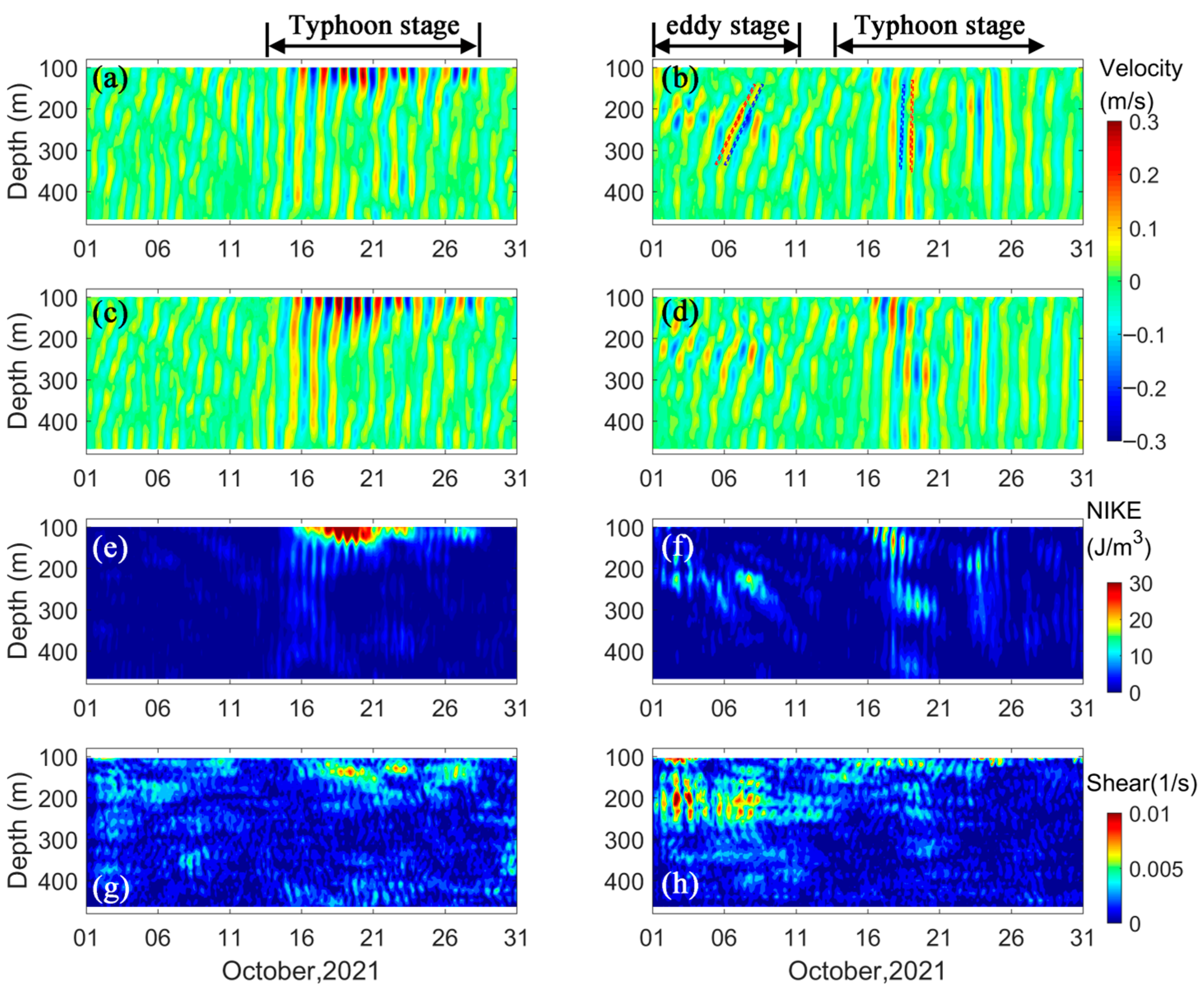
2.5. Bandpass Filtering, Near-Inertial Kinetic Energy, and Near-Inertial Velocity Shears

Anomalous values in the raw current data were removed, after which linear interpolation methods were used to convert the data to a specified depth, to obtain continuous ocean currents at the same depth. The focus of this study was on NIWs. Near-inertial velocities (u_f, v_f) were obtained using a fourth-order Butterworth bandpass method. The cutoff frequency band was [0.8, 1.2] f₀, where f₀ is the local inertial frequency.

The near-inertial kinetic energy density (NIKE) can be calculated from the near-inertial velocities using Equation (1):

$$NIKE=\frac{1}{2}\rho \left(z\right)\left(u_f^2+v_f^2\right)$$

(1)

where $\rho \left(z\right)$ is the seawater density calculated from CTD data by glider measurements, and $u_f$ and $v_f$ are the zonal and meridional near-inertial velocities, respectively.

The near-inertial velocity shears were calculated as

$$S=\sqrt{{\left|\frac{\partial u_f}{\partial z}\right|}^2+{\left|\frac{\partial v_f}{\partial z}\right|}^2}$$

(2)

2.6. Gregg–Henyey–Polzin Parameterization

Gregg–Henyey–Polzin (GHP) parameterization was applied to estimate the enhanced mixing induced by NIWs. GHP parameterization is a commonly used method for quantifying ocean turbulence from CTD measurements [23,24]. It is based on the theory of internal wave–wave interactions and was first developed by Wijesekera et al. [25]. In this study, GHP parameterization was employed to determine the diapycnal diffusivities based on the glider’s CTD measurements. The GHP is calculated according to Equations (3)–(5):

$$K_{\rho }=K_0\frac{{\langle {\xi }_z^2\rangle }^2}{{}_{GM}{\langle {\xi }_z^2\rangle }^2}h\left(R_w\right)j\left(\frac{f}{N}\right)$$

(3)

$$h\left(R_w\right)=\frac{1}{6\sqrt{2}}\frac{R_w\left(R_w+1\right)}{\sqrt{R_w-1}}$$

(4)

$$j\left(\frac{f}{N}\right)=\frac{farccosh\left(N/f\right)}{f_{30}arccosh\left(N/f\right)}$$

(5)

where K₀ = 5 × 10⁻⁶ m²/s, $\langle {\xi }_z^2\rangle$ is the observations-inferred fine-scale internal wave strain variance and ${}_{GM}\langle {\xi }_z^2\rangle$ is the Garrett and Munk (GM) spectrum-inferred strain variance [26]. The GM model assumes a fixed buoyancy frequency (N₀ = 5.2 × 10⁻³ 1/s) at a latitude of 30° in an open-ocean internal wave field. The functions f and N are the Coriolis and buoyancy frequencies, respectively, and R_ω is the shear/strain variance ratio. R_ω was set to 7 as suggested by Kunze et al. [24]. This value was later used by Yang et al. [27] to quantify mixing in the SCS. To quantify strain $\langle {\xi }_z^2\rangle$, the glider profiles were first divided into semi-overlapping 300 m long segments, starting from the bottom and excluding data from the surface mixed layer.

The internal wave strain was estimated as ${\xi }_z=\left(N^2-\overline{N^2}\right)/\overline{N^2}$, where $\overline{N^2}$ is the mean value inferred from quadratic fitting to each busoyancy frequency segment. Strain variance was calculated as $\langle {\xi }_z^2\rangle ={{\displaystyle \int }}_{\min \left(k_z\right)}^{\max \left(k_z\right)}S\left[{\xi }_z\right]\left(k_z\right)\mathrm{d}{k}_z$. A minimum integrated wavenumber of 0.042 rad/m, corresponding to a vertical wavelength λ_z = 150 m, was used to integrate the strain variance; the lower wavenumber reflects the influence of strong background stratification in the pycnocline [24,28]. The upper boundary integrated wavenumber was set at 0.419 rad/m and corresponded to a vertical wavelength of λ_z = 15 m. The GM strain variance was calculated over the same wavenumber band using Equation (6):

$${}_{GM}\langle {\xi }_z^2\rangle =\frac{\pi E_{0}b{j}_{*}}{2}{{\displaystyle \int }}_{\min \left(k_z\right)}^{\max \left(k_z\right)}\frac{k^2}{\left(k+k_{*}\right)}\mathrm{d}{k}_z$$

(6)

where E₀ = 6.3 × 10⁻⁵ is the dimensionless energy level; $j_{*}$ = 3 is the reference mode number; b = 1300 m is the scale depth of the thermocline; and $k_{*}=\left(\pi j_{*}N\right)/\left(b{N}_0\right)$ is the reference wavenumber.

Although the glider was operated in a mode of virtual anchoring, it should be noted that the glider glided under water at a certain angle of inclination, meaning the glider could have observed a horizontal wave number component of internal waves which could contaminate the strain parameterization. This aspect requires further study, which goes beyond the scope of this paper.

3. Results

3.1. Characteristics of the Observed NIWs

The observed NIWs differed significantly between the two moorings. For mooring A (shelf break region), before typhoon “Kompasu” passed through the mooring array, from 1 October to 11 October, the near-inertial velocities were small (<0.1 m/s; Figure 4). After the typhoon, the near-inertial velocities were significantly enhanced at both moorings, with a maximum velocity of >0.3 m/s lasting for 2 weeks. At mooring A, strong NIWs appeared in the upper 200 m, whereas at deeper depths the near-inertial energy decreased rapidly. A typical upward phase propagation and downward energy propagation were also recorded (Figure 4a,c).

At mooring B (deep water region), smaller but still significant velocity amplitudes were recorded in two main depth ranges of 100~200 m and 250~350 m between 16 October and 21 October (Figure 4f). And then, after 22 October, NIKE signals were found between 150 and 400 m. The differences between the two moorings were caused by differences in their positions and the typhoon’s path (Figure 1a). The center of the typhoon passed through mooring A whereas mooring B was located ~140 km away from the nearest typhoon path. The two moorings were within and outside the maximum wind radius of 97 km/h, respectively.

Before the typhoon event, during the mesoscale eddy stage from 1 to 11 October, remarkable NIWs with a maximum velocity of >20 cm/s occurred at depths of 150–300 m (Figure 4b,d). This depth range represented the lower boundary of the anticyclonic eddy and the location of the peak values of buoyancy frequency (Figure 3b). At this stage, mooring B captured an anticyclonic mesoscale eddy that moved and deformed, such that it eventually moved away from the mooring (Figure 1b,c). During the same period, similar NIW signals were not recorded at mooring A at any depth (Figure 4a,c). A the same time, the sea surface wind was moderate at ~10 m/s (Figure 2). These results suggested that the NIWs captured by mooring B limited at depths of 150–300 m during 1–11 October were trapped by the anticyclonic mesoscale eddy. A notable feature at the eddy stage was the much steeper phase of the NIWs than at the typhoon stage, as the dash lines shown in Figure 4b. At the eddy stage, the inertial phase becomes $\mathsf{\pi }$/2 relative to the inertial current vector was approximately 40 m, meaning the vertical scales of NIWs were about 80 m. While at the typhoon stage, Figure 4b can not figure out the vertical difference of the inertial phase. This difference implied that, at the eddy stage, the NIWs in the downward phase of propagation likely had shorter vertical scales or higher wavenumbers, either of which might have effectively contributed to turbulent mixing.

Before typhoon “Kompasu”, from 1 October to 11 October, near-inertial velocity shears at mooring A were hardly recognizable, with a maximum value of 0.005 1/s (Figure 4g). Moderate winds of ~10 m/s caused by the winter monsoon in the northern SCS before the arrival of “Kompasu” at the mooring array may have induced weak NIWs at the moorings. Although slightly higher winds of ~12 m/s were recorded after “Kompasu”, it is reasonable to believe the recognizable NIWs at the moorings were not caused by winter monsoon but by typhoon “Kompasu”. The shears have been elevated > 2-fold after the transit of “Kompasu” (Figure 4g). The elevated shears were mainly confined to the upper 200 m, with the near-inertial velocity magnitude below 200 m being slightly weaker than that above 200 m (Figure 4a,c). For mooring B, significantly enhanced shears appeared at the eddy stage at depths of 150–300 m (Figure 4h). At the typhoon stage, the shears were much weaker, although the near-inertial velocity magnitude was comparable to that at the eddy stage (Figure 4b,d), suggesting shorter vertical scales of the NIWs at the eddy stage than at the typhoon stage. The near-inertial velocity shears may have ultimately extracted and dissipated the wave energy [29,30], which would have resulted in turbulence and related vertical mixing.

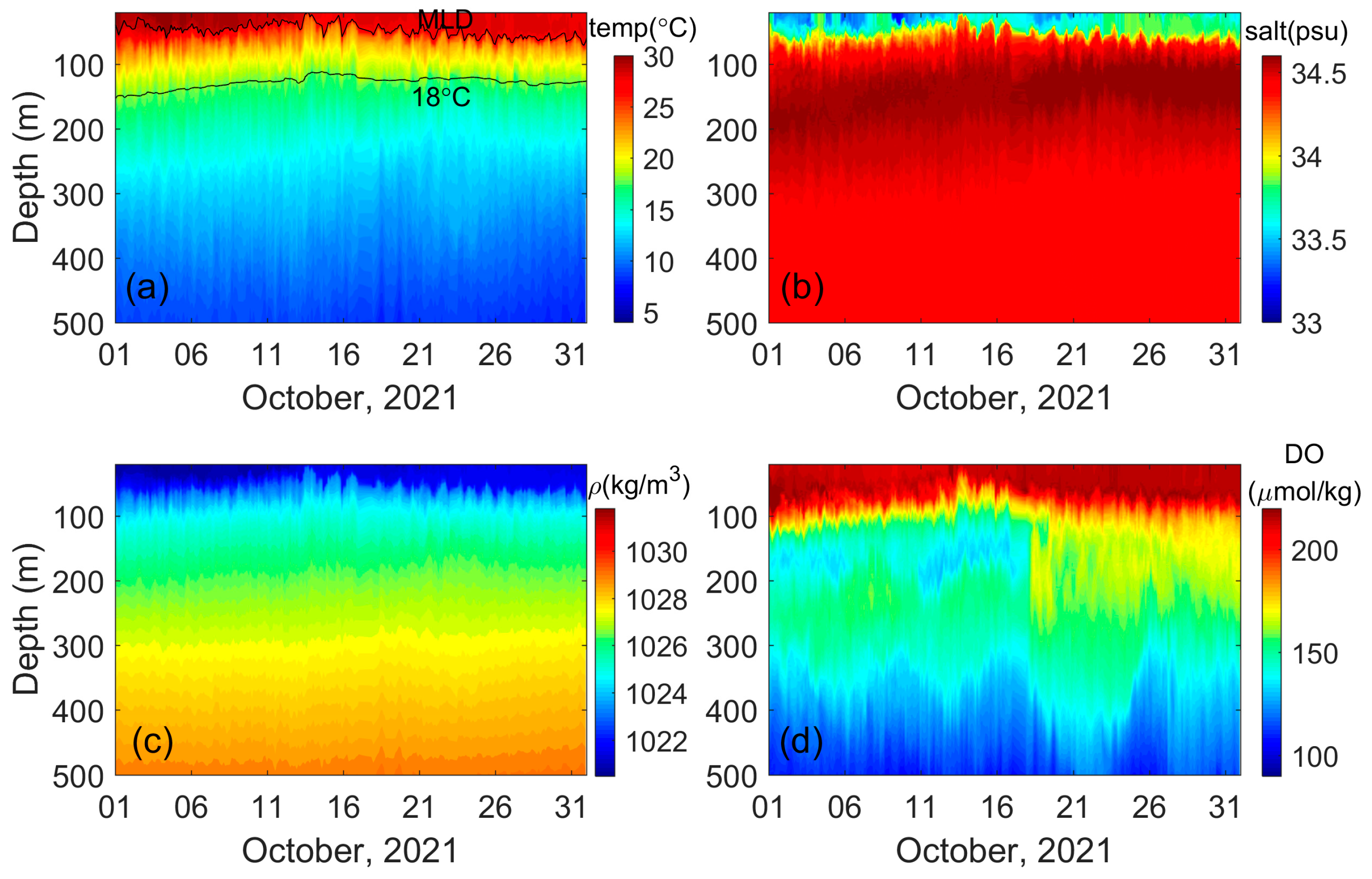
3.2. Glider Observations

The surface positions of the glider were within a range of 5 km, indicating that the ocean environmental changes observed by the glider represented the changes that occurred at fixed points. Figure 5 shows the time-depth graph of glider-observed temperature, salinity, density, and DO in the upper 500 m. From 1 to 11 October, the water column was affected by the anticyclonic eddy, evidenced by the depth corresponding to the 18° isotherm (Figure 5a). The accumulation of warm water at the center of the anticyclonic eddy caused an isothermal and isosalinity downforce (Figure 5a,b), and so does the density section (Figure 5c).

Figure 6 shows the averaged vertical profiles of temperature, salinity, and DO in the upper 500 m of the water column as recorded by the glider during the periods 1–11 October, 12–17 October, and 18–31 October. The vertical profiles of the observed temperature and salinity indicated upwelling during typhoon “Kompasu” on 12–17 October that brought deep subsurface waters (between ~30 and 100 m) of low temperature and high salinity to the shallow layer on 12–17 October (Figure 6a,b). This upwelling was verified by the variation in the averaged MLD for the upper water column. During 1–11 October, i.e., the eddy stage, the MLD was ~35 m, but during 12–17 October it decreased to 24 m. During 18–31 October, after the transit of typhoon “Kompasu”, the MLD increased to 42 m. The DO concentrations decreased significantly at depths < 160 m (with a maximum decrease of 25 μmol/kg at 76 m) between 1–11 October and 12–17 October 2021. After the transit of typhoon “Kompasu”, during 18–31 October, the DO concentrations returned to the pre-storm level in the upper ~100 m but increased significantly at 100–250 m depth, with a maximum decrease of 30 μmol/kg at 150 m.

3.3. Enhanced Mixing

A section of inferred diffusivity ($\kappa$) based on the GHP parameterization, including the temporal and spatial variations, is shown in Figure 7a. In general, the diffusivity decreased as the depth increased. The diffusivity values ranged from a minimum of <10⁻⁵ m²/s to a maximum of 10⁻² m²/s. High-level mixing and diffusivity values of the order of 10^–2 m²/s were determined at depths < 300 m. Both the eddy stage and the typhoon stage were characterized by peaks in diffusivity. For example, the average diffusivity on 3 October reached 10^–2 m²/s, while during 11–13 October, it was an order of magnitude smaller (Figure 7a).

Shear [31] and convective instability [32,33,34], in which steep internal waves cause an overturning of the crests, can generate ocean turbulent mixing. To investigate further the relationship between shear and diffusivity, the shear obtained from each mooring and the diffusivity obtained from the glider were averaged for depths < 300 m (Figure 7b). At mooring A, high shear values characterized the typhoon stage, while at mooring B, the values were highest during the eddy stage. At the same time, peaks of diffusivity appeared. It should be noted that the position difference between the moorings and the glider was relatively large and that the glider was located between the two moorings. Nonetheless, there was a significant positive correlation between shear and diffusivity.

4. Discussion

Near-inertial waves (NIWs), or waves within 20–30% of the local inertial frequency f [35], contain a significant amount of internal wave energy and ocean shear forces [36,37]. In the ocean’s interior, because of their greater shear/strain ratio and their variance at small vertical scales, NIWs may be more effective at mixing than internal tides. An enhanced dissipation associated with NIWs has been described in the Arctic [38,39,40]. Other evidence for the universal importance of NIWs in upper ocean mixing comes from an analysis of the parameterized diffusivities in the upper 500 m, estimated from Argo floats using the Gregg–Henyey strain formulation [41,42]. That study found strong seasonal cycles in certain latitude zones, with much higher parameterized mixing in winter, consistent with the ability of storm-generated NIWs to enhance mixing. In this study, significant NIWs were observed, and their energy during the typhoon stage significantly increased. The energy of the sea surface wind field propagated toward the deep sea in the form of NIWs, accompanied by significantly increased ocean mixing, thus providing further evidence of enhanced ocean mixing by NIWs.

Enhanced inertial pumping also occurs in the presence of mesoscale eddies [43]. The horizontal spatial scale of NIWs is on the order of 10–100 km, similar to the spatial scale of mesoscale eddies. The slow group velocities of NIWs favor their strong interaction with mesoscale features in the ocean. This interaction can take several forms, including mesoscale effects on wind generation, the refraction and capture of propagating waves, and two-way nonlinear energy transfers with mesoscale and submesoscale features [9]. Both the trapping and the accumulation of near-inertial energy in anticyclonic eddies have been documented [44,45]. By contrast, near-inertial oscillations originating from the interior of a cyclone are not trapped but, instead, rapidly propagate into the deeper ocean [46,47]. In this study, a significant near-inertial velocity shear was observed at the eddy stage, during 1–11 October, at mooring B, with a main impact depth of 150–300 m (Figure 4f,h). This depth was the base region affected by the eddy. After 11 October, the area affected by the mesoscale eddy moved away from mooring B and the high shear at the base of the eddy disappeared. This study is the first to report NIWs trapped by anticyclonic mesoscale eddies, and causing strong mixing in the SCS.

NIWs are a major contributor to upper-ocean mixing and thus also affect a variety of processes, including those related to biogeochemistry and climate [48]. The wind stress curl caused by typhoons generates vertical mixing and upwelling within the ocean, leading to a deepening of the mixing layer. When typhoon-driven mixing breaks through the MLD, it provides nutrient-rich water from the upper ocean and thus promotes phytoplankton growth, detected as a significant increase in the chlorophyll concentration. Intense tropical cyclones have been shown to play a critical role in DO distribution in the surface waters of deep oceans and coastal waters [49,50,51,52]. For example, Chen et al. [49] reported that, after typhoon “Muifa”, mixing in the Changjiang Estuary caused DO concentrations to remain high for 6–8 days. Xu et al. [53] reported three types of DO temporal variability caused by storm-induced mixing and upwelling. In this study, after the typhoon had passed through the study area, the DO content at different depths increased (Figure 4d). The changes in the DO concentration after the typhoon can be seen in the averaged vertical profiles of 1–17 October and 18–31 October (Figure 6c). Considering the changes in the DO concentration throughout the water column, the average DO concentration during 18–31 October was 5 $\mathsf{\mu }\mathrm{mol}/\mathrm{kg}$ higher than during 12–17 October. The largest increment occurred at a depth of 150 m, where the average DO increased from 140 $\mathsf{\mu }\mathrm{mol}/\mathrm{kg}$ to 164 $\mathsf{\mu }\mathrm{mol}/\mathrm{kg}$, likely due to storm-induced mixing.

Not all strong mixing causes significant changes in the DO concentration. Despite strong mixing and high near-inertial shears at the eddy stage (1–11 October), there were no corresponding changes in DO (Figure 5d), because the strong mixing and high near-inertial shears induced by the anticyclonic eddy were limited to depths of 150–300 m, which was deeper than the base of the surface mixed layer. As a result, water with a high DO on the surface remained isolated. After the typhoon, the near-inertial velocity extended from the surface to the deep sea, accompanied by strong mixing (Figure 4b,d,f and Figure 6a), such that DO increase.

5. Conclusions

Observations acquired from two moorings and a glider in the northern SCS were used to analyze the enhanced mixing induced by NIWs in response to an anticyclonic eddy and typhoon “Kompasu”. The moorings differed in their locations and responded differently to the eddy and the typhoon. At mooring B, significant NIWs at the base of the eddy were limited to a depth range of 150–300 m on 1–11 October 2021, whereas the typhoon (18–31 October 2021) triggered stronger NIWs that extended to depths > 500 m. Our observations provide evidence for the trapping of NIW packets of amplitude ~0.2 m/s near the base of an anticyclonic eddy, and of amplitude ~0.3 m/s after the transit of typhoon “Kompasu”. The observed upward phase propagation (downward energy propagation) suggested that the NIWs were generated at the surface. The higher near-inertial velocity shears at the eddy-impacted stage than at the typhoon-impacted stage indicated the shorter vertical scales of NIWs trapped at the base of the eddy. Richardson numbers ≤ 1 indicated that these trapped NIWs enhanced the turbulence near the base of the eddy and after the typhoon event, evidenced by the GHP parameterization of the turbulence. The parameterized diffusivity reached 10⁻² m²/s at the base of the eddy (100–300 m) and after the typhoon event, while during other periods the averaged diffusivity was one order of magnitude smaller. This study therefore showed that NIWs are an important pathway for ocean energy transmission. They also serve as a bridge between mesoscale eddies and small-scale motion and are thus able to promote the forward transfer of mesoscale eddy energy effectively to small-scale motions. Anticyclonic mesoscale eddies in the northern SCS may act as deep mixing structures as they propagate to the west. Further microstructure studies and high-resolution sampling within mesoscale eddies and after typhoon events are necessary to quantify the energetics transfer and their impacts at regional scales.

References

1. Chelton, D.B.; Schlax, M.G.; Samelson, R.M. Global observations of nonlinear mesoscale eddies. Prog. Oceanogr. 2011, 91, 167–216. [Google Scholar] [CrossRef]
2. Munk, W. Abyssal recipes. Deep-Sea Res. 1966, 13, 707–730. [Google Scholar] [CrossRef]
3. Alford, M.H.; MacKinnon, J.A.; Simmons, H.L.; Nash, J.D. Near-inertial internal gravity waves in the ocean. Ann. Rev. Mar. Sci. 2016, 8, 95–123. [Google Scholar] [CrossRef]
4. Munk, W.; Wunsch, C. Abyssal recipes II: Energetics of tidal and wind mixing. Deep-Sea Res. Pt I 1998, 45, 1977–2010. [Google Scholar] [CrossRef]
5. Park, J.J.; Kim, K.; King, B.A. Global statistics of inertial motions. Geophys. Res. Lett. 2005, 32, L14612. [Google Scholar] [CrossRef]
6. Park, J.J.; Kim, K.; Schmitt, R.W. Global distribution of the decay time scale of mixed layer inertial motions observed by satellite tracked drifters. J. Geophys. Res. 2009, 114, C11010. [Google Scholar] [CrossRef]
7. Wunsch, C.; Ferrari, R. Vertical mixing, energy, and the general circulation of the oceans. Ann. Rev. Fluid Mech. 2004, 36, 281–314. [Google Scholar] [CrossRef]
8. Martínez-Marrero, A.; Barceló-Llull, B.; Pallàs-Sanz, E.; Aguiar-González, B.; Estrada-Allis, S.N.; Gordo, C.; Grisolía, D.; Rodríguez-Santana, A.; Arístegui, J. Near-inertial wave trapping near the base of an anticyclonic mesoscale eddy under normal atmospheric conditions. J. Geophys. Res.-Oceans 2019, 124, 8455–8467. [Google Scholar] [CrossRef]
9. Byun, S.S.; Park, J.J.; Chang, K.I.; Schmitt, R.W. Observation of near- inertial wave refections within the thermostad layer of an anticyclonic mesoscale eddy. Geophys. Res. Lett. 2010, 37, 1–6. [Google Scholar] [CrossRef]
10. Xie, S.; Xie, Q.; Wang, D.; Liu, W.T. Summer up welling in the South China Sea and its role in regional climate variations. J. Geophys. Res.-Oceans 2003, 108, 3261. [Google Scholar] [CrossRef]
11. Qu, T. Upper-layer circulation in the South China Sea. J. Phys. Oceanogr. 2000, 30, 1450–1460. [Google Scholar] [CrossRef]
12. Wang, G.; Xie, S.; Qu, T.; Huang, R.X. Deep South China Sea circulation. Geophys. Res. Lett. 2011, 38, L05601. [Google Scholar] [CrossRef]
13. Alford, M.H.; Peacock, T.; Mackinnon, J.M.; Nash, J.D.; Buijsman, M.C.; Centurioni, L.R.; Chao, S.-Y.; Chang, M.-H.; Farmer, D.M.; Fringer, O.B.; et al. The formation and fate of internal waves in the South China Sea. Nature 2015, 521, 65–69. [Google Scholar] [CrossRef] [PubMed]
14. Huang, X.; Chen, Z.; Zhao, W.; Zhang, Z.; Zhou, C.; Yang, Q.; Tian, J. An extreme internal solitary wave event observed in the northern South China Sea. Sci. Rep.-UK 2016, 6, 30041. [Google Scholar] [CrossRef] [PubMed]
15. Tian, J.; Yang, Q.; Zhao, W. Enhanced diapycnal mixing in the South China Sea. J. Phys. Oceanogr. 2009, 39, 3191–3203. [Google Scholar] [CrossRef]
16. Liang, C.; Chen, G.; Shang, X. Observa tions of the turbulent kinetic energy dissipation rate in the upper central South China Sea. Ocean Dynam. 2017, 67, 597–609. [Google Scholar] [CrossRef]
17. Zhang, Z.; Zhao, W.; Tian, J.; Liang, X. A mesoscale eddy pair southwest of Taiwan and its influence on deep circulation. J. Geophys. Res.-Oceans 2013, 118, 6479–6494. [Google Scholar] [CrossRef]
18. Qiu, C.; Mao, H.; Liu, H.; Xie, Q.; Yu, J.; Su, D.; Ouyang, J.; Lian, S. Deformation of a warm eddy in the northern South China Sea. J. Geophys. Res.-Oceans 2019, 124, 5551–5564. [Google Scholar] [CrossRef]
19. Qi, Y.; Mao, H.; Wang, X.; Yu, L.; Lian, S.; Li, X.; Shang, X. Suppressed Thermocline Mixing in the Center of Anticyclonic Eddy in the North South China Sea. J. Mar. Sci. Eng. 2021, 9, 1149. [Google Scholar] [CrossRef]
20. Qi, Y.; Mao, H.; Du, Y.; Li, X.; Yang, Z.; Xu, K.; Yang, Y.; Zhong, W.; Zhong, F.; Yu, L.; et al. A lens-shaped, cold core anticyclonic surface eddy in the northern South China Sea. Front. Mar. Sci. 2022, 9, 976273. [Google Scholar] [CrossRef]
21. Zhang, H.; Liu, X.; Wu, R.; Chen, D.; Zhang, D.; Shang, X.; Wang, Y.; Song, X.; Jin, W.; Yu, L.; et al. Sea surface current response patterns to tropical cyclones. J. Mar. Syst. 2020, 208, 103345. [Google Scholar] [CrossRef]
22. Zhang, H.; Liu, X.; Wu, R.; Liu, F.; Yu, L.; Shang, X.; Qi, Y.; Wang, Y.; Song, X.; Xie, X.; et al. Ocean Response to Successive Typhoons Sarika and Haima (2016) Based on Data Acquired via Multiple Satellites and Moored Array. Remote Sens. 2019, 11, 2360. [Google Scholar] [CrossRef]
23. Gregg, M.C.; Sanford, T.B.; Winkel, D.P. Reduced mixing from the breaking of internal waves in equatorial waters. Nature 2003, 422, 513–515. [Google Scholar] [CrossRef]
24. Kunze, E.; Firing, E.; Hummon, J.M.; Chereskin, T.K.; Thurnherr, A.M. Global abyssal mixing inferred from lowered ADCP shear and CTD strain profiles. J. Phys. Oceanogr. 2006, 36, 1553–1576. [Google Scholar] [CrossRef]
25. Wijesekera, H.; Padman, L.; Dillon, T.; Levine, M.; Paulson, C.; Pinkel, R. The application of internal-wave dissipation models to a region of strong forcing, J. Phys. Oceanogr. 1993, 23, 269–286. [Google Scholar] [CrossRef]
26. Garrett, C.; Munk, W. Space-time scales of internal waves: A progress report. J. Geophys. Res. 1975, 80, 291–297. [Google Scholar] [CrossRef]
27. Yang, Q.; Zhao, W.; Liang, X.; Tian, J. Three-dimensional distribution of turbulent mixing in the South China Sea. J. Phys. Oceanogr. 2016, 46, 769–788. [Google Scholar] [CrossRef]
28. Jing, Z.; Wu, L. Low-frequency modulation of turbulent diapycnal mixing by anticyclonic eddies inferred from the HOT time series. J. Phys. Oceanogr. 2013, 43, 824–835. [Google Scholar] [CrossRef]
29. Xie, X.; Shang, X.; Chen, G.; Sun, L. Variations of diurnal and inertial spectral peaks near the bi-diurnal critical latitude. Geophys. Res. Lett. 2009, 36, 349–363. [Google Scholar] [CrossRef]
30. Zhang, S.; Xie, L.; Hou, Y.; Zhao, H.; Qi, Y.; Yi, X. Tropical storm-induced turbulent mixing and chlorophyll-a enhancement in the continental shelf southeast of Hainan Island. J. Mar. Syst. 2014, 129, 405–414. [Google Scholar] [CrossRef]
31. Kundu, P.K.; Beardsley, R.C. Evidence of a critical Richardson number in moored measurements during the upwelling season off Northern California. J. Geophys. Res. 1991, 96, 4855–4868. [Google Scholar] [CrossRef]
32. Munk, W. Internal waves and small-scale processes. In Evolution of Physical Oceanography; Warren, B.A., Wunsch, C., Eds.; MIT Press: Cambridge, MA, USA, 1981; pp. 264–291. [Google Scholar]
33. Thorpe, S.A. On the shape and breaking of finite amplitude internal gravity waves in a shear flow. J. Fluid Mech. 1978, 85, 7–31. [Google Scholar] [CrossRef]
34. Canuto, V.M.; Howard, A.; Cheng, Y.; Dubovikov, M.S. Ocean turbulence. Part I: One-point closure model-momentum and heat vertical diffusivities. J. Phys. Oceanogr. 2001, 31, 1413–1426. [Google Scholar] [CrossRef]
35. Garrett, C. What is the “near-inertial” band and why is it different from the rest of the internal wave spectrum? J. Phys. Oceanogr. 2001, 31, 962–971. [Google Scholar] [CrossRef]
36. Alford, M.H.; MacKinnon, J.A.; Pinkel, R.; Klymak, J.M. Space-time scales of shear in the North Pacific. J. Phys. Oceanogr. 2017, 47, 2455–2478. [Google Scholar] [CrossRef]
37. Weller, R.A. The relation of near-inertial motions observed in the mixed layer during the JASIN (1978) Experiment to the local wind stress and to the quasi-geostrophic flow field. J. Phys. Oceanogr. 1982, 12, 1122–1136. [Google Scholar] [CrossRef]
38. Fer, I. Near-inertial mixing in the Central Arctic Ocean. J. Phys. Oceanogr. 2014, 44, 2031–2049. [Google Scholar] [CrossRef]
39. Hebert, D.; Moum, J.N. Decay of a near-inertial wave. J. Phys. Oceanogr. 1994, 24, 2334–2351. [Google Scholar] [CrossRef]
40. Alford, M.H.; Gregg, M.C. Near-inertial mixing: Modulation of shear, strain and microstructure at low latitude. J. Geophys. Res.-Oceans 2001, 106, 16947–16968. [Google Scholar] [CrossRef]
41. Whalen, C.B.; Talley, L.D.; MacKinnon, J.A. Spatial and temporal variability of global ocean mixing inferred from Argo profiles. Geophys. Res. Lett. 2012, 39, L18612. [Google Scholar] [CrossRef]
42. Whalen, C.B.; MacKinnon, J.A.; Talley, L.D.; Waterhouse, A.F. Estimating the mean diapycnal mixing using a finescale strain parameterization. J. Phys. Oceanogr. 2015, 45, 1174–1188. [Google Scholar] [CrossRef]
43. van Meurs, P. Interactions between near-inertial mixed layer currents and the mesoscale: The importance of spatial variabilities in the vorticity field. J. Phys. Oceanogr. 1998, 28, 1363–1388. [Google Scholar] [CrossRef]
44. Kunze, E.; Schmitt, R.W.; Toole, J.M. The energy balance in a warm-core ring’s near-inertial critical layer. J. Phys. Oceanogr. 1995, 25, 942–957. [Google Scholar] [CrossRef]
45. Joyce, T.M.; Toole, J.M.; Klein, P.; Thomas, L.N. A near-inertial mode observed within a Gulf Stream warm-core ring. J. Geophys. Res.-Oceans 2013, 118, 1797–1806. [Google Scholar] [CrossRef]
46. Kunze, E. Near-inertial wave propagation in geostrophic shear. J. Phys. Oceanogr. 1985, 15, 544–565. [Google Scholar] [CrossRef]
47. Lee, D.K.; Niiler, P.P. The inertial chimney: The near inertial energy drainage from the ocean surface to the deep layer. J. Geophys. Res. 1998, 103, 7579–7591. [Google Scholar] [CrossRef]
48. Jochum, M.; Briegleb, B.P.; Danabasoglu, G.; Large, W.G.; Jayne, S.R.; Alford, M.H.; Bryan, F.O. On the impact of oceanic nearinertial waves on climate. J. Clim. 2012, 26, 2833–2844. [Google Scholar] [CrossRef]
49. Chen, Y.; Tang, D. Eddy-feature phytoplankton bloom induced by a tropical cyclone in the South China Sea. Int. J. Remote Sens. 2012, 33, 7444–7457. [Google Scholar] [CrossRef]
50. Feng, Y.; DiMarco, S.F.; Jackson, G.A. Relative role of wind forcing and riverine nu trient input on the extent of hypoxia in the northern Gulf of Mexico. Geophys. Res. Lett. 2012, 39. [Google Scholar] [CrossRef]
51. Lin, J.; Tang, D.; Alpers, W.; Wang, S. Response of dissolved oxygen and related ma rine ecological parameters to a tropical cyclone in the South China Sea. Adv. Space Res. 2014, 53, 1081–1091. [Google Scholar] [CrossRef]
52. Wang, B.; Chen, J.; Jin, H.; Li, H.; Huang, D.; Cai, W.J. Diatom bloom-derived bottom water hypoxia off the Changjiang estuary, with and without typhoon influence. Limnol. Oceanogr. 2017, 62, 1552–1569. [Google Scholar] [CrossRef]
53. Xu, H.B.; Tang, D.L.; Sheng, J.Y.; Liu, Y.P.; Sui, Y. Study of dissolved oxygen responses to tropical cyclones in the Bay of Bengal based on Argo and satellite observations. Sci. Total Environ. 2019, 659, 912–922. [Google Scholar] [CrossRef] [PubMed]
Figure 1. (a) Map showing the observation position and trajectory of typhoon “Kompasu”. The two moorings (A and B) are labeled with white stars. The diamonds indicate the glider operation positions. The red and blue dashed circles indicate the wind radii (50 knots and 34 knots, respectively) at 21:00 on 12 October 2021, and the filled color circles the maximum wind speed. The inlet in (a) is the surface position relative to the center position; (b,c) are the sea level anomaly on 1 October 2021 and 18 October 2021, respectively. (d) The two mooring systems and ‘Sea-wing’ Glider diagrammatic sketch.
Jmse 11 02141 g001
Figure 2. Time series of daily winds at Mooring B from ASCAT scatterometers (http://marine.copernicus.eu, accessed on 1 October 2023). The data on 10–11 October were missed.
Jmse 11 02141 g002
Figure 3. (a) Map of MODIS 8-day (16–23 October 2021) composite SST in the northern South China Sea. The black lines denote the sea level anomaly on 18 October 2021. (b) Longitude-depth plot of the squared Brunt–Vaisala Frequency at 17.75° N on 1 October 2021 calculated with datasets of the global ocean physics analysis and forecast system distributed by the CMEMS. The surface mixed layer depth (MLD) and plots of temperature were marked with dense lines and thin lines, respectively.
Jmse 11 02141 g003
Figure 4. Time-depth graph of the band-pass ([0.8, 1.2] f0)-filtered near-inertial (meridional and zonal) velocities (a,c), the moving-average near-inertial kinetic energy density (e), and the near-inertial velocity shear from 1 to 31 October 2021, at mooring A. Panels (b,d,f,h) are the same as panels (a,c,e,g) but for mooring B. The eddy stage and typhoon stage are marked. In (b), the dash lines indicate the phase propagation of inertial currents.
Jmse 11 02141 g004
Figure 5. Time-depth graph of the underwater-glider-observed temperature (a), salinity (b), density (c), and DO (d). The surface mixed layer depth and isotherm of 18 °C are shown in (a).
Jmse 11 02141 g005
Figure 6. Averaged vertical profiles of the glider-observed temperature (a), salinity (b), and DO (c) in the upper 500 m of the water column during 1–11 October, 12–17 October, and 18–31 October.
Jmse 11 02141 g006
Figure 7. Time-depth graph of diffusivity as derived from glider observations (a). Average shear at depths < 300 m, obtained at mooring A and mooring B, the corresponding profile average and daily average diffusivity obtained from glider observations (b).
Jmse 11 02141 g007
Disclaimer/Publisher’s Note: The statements, opinions and data contained in all publications are solely those of the individual author(s) and contributor(s) and not of MDPI and/or the editor(s). MDPI and/or the editor(s) disclaim responsibility for any injury to people or property resulting from any ideas, methods, instructions or products referred to in the content.